Attenuation of Tides and Surges by Mangroves: Contrasting Case Studies from New Zealand


Faculty of Science and Engineering, School of Science, University of Waikato, Private Bag 3105, Hamilton 3240, New Zealand
*
Author to whom correspondence should be addressed.
Water 2018, 10(9), 1119; https://doi.org/10.3390/w10091119
Submission received: 29 June 2018
/
Revised: 17 August 2018
/
Accepted: 17 August 2018
/
Published: 23 August 2018
(This article belongs to the Special Issue Coastal Vulnerability and Mitigation Strategies: From Monitoring to Applied Research
)
Abstract
:Mangroves have been suggested as an eco-defense strategy to dissipate tsunamis, storm surges, and king tides. As such, efforts have increased to replant forests along coasts that are vulnerable to flooding. The leafy canopies, stems, and aboveground root structures of mangroves limit water exchange across a forest, reducing flood amplitudes. The attenuation of long waves in mangroves was measured using cross-shore transects of pressure sensors in two contrasting environments in New Zealand, both characterized by mono-specific cultures of grey mangroves (Avicennia marina) and approximate cross-shore widths of 1 km. The first site, in the Firth of Thames, was characterized by mangrove trees with heights between 0.5 and 3 m, and pneumatophore roots with an average height of 0.2 m, and no substantial tidal drainage channels. Attenuation was measured during storm surge conditions. In this environment, the tidal and surge currents had no alternative pathway than to be forced into the high-drag mangrove vegetation. Observations showed that much of the dissipation occurred at the seaward fringe of the forest, with an average attenuation rate of 0.24 m/km across the forest width. The second site, in Tauranga harbor, was characterized by shorter mangroves between 0.3 and 1.2 m in height and deeply incised drainage channels. No attenuation of the flood tidal wave across the mangrove forest was measurable. Instead, flow preferentially propagated along the unvegetated low-drag channels, reaching the back of the forest much more efficiently than in the Firth of Thames. Our observations from sites with the same vegetation type suggest that mangrove properties are important to long wave dissipation only if water transport through the vegetation is a dominant mechanism of fluid transport. Therefore, realistic predictions of potential coastal protection should be made prior to extensive replanting efforts.
1. Introduction
Mangroves are the dominant species of vegetation in many tropical and sub-tropical intertidal environments. These salt-tolerant trees provide a valuable habitat for a range of animal species, reduce hydrodynamic forces, promote sedimentation, and provide protection from floods [1]. Additionally, mangroves are significantly more efficient than many terrestrial ecosystems at sequestering carbon [2]. Mangroves thrive in the zone between mean sea-level and high water and thus are sensitive to changes in inundation regime. Their zonation and ability to prevent erosion or increase sedimentation may provide a mechanism for mangroves to adapt to sea level rise and alleviate the threat of coastal retreat [3]. Despite the diverse array of valuable services, worldwide mangrove populations are in steep decline, with the loss of over one-quarter of global mangrove cover since 1980 [1,4].
Extreme flooding events are projected to increase with sea level rise [5,6]. Additionally, coastal populations and infrastructure are increasing [7], driving demand for effective coastal protection. Conventional engineering solutions are often costly and may have a limited lifespan, destroy or fragment sensitive habitat, and have been associated with enhanced erosion [8,9]. Coastal vegetation has been proposed as an alternative to hard engineering solutions. Mangroves can provide coastal protection by reducing storm waves, dissipating currents, and stabilizing sediments [10,11]. Additionally, sedimentation in mangrove forests may provide a mechanism to maintain present coastlines with respect to sea level rise [12].
The reduction in the wave height of short period wind-generated waves due to interaction with mangroves is well established [10,13,14]. Less well established are the protective benefits of mangroves with respect to storm surge [15,16,17]. Mangroves reduce peak flood levels by limiting fluid exchange across the forest [18]. Dissipation of storm surges through coastal vegetation has previously been quantified as a reduction in peak water level (cm) per distance of flood propagation (km) with values categorized by vegetation type [15,16,17,18]. Although providing an easily accessible solution, using fixed dissipation rates over wide-ranging sites may oversimplify flood protection provided by coastal vegetation.
Alongi [12] noted that flood protection provided by coastal vegetation is dependent on vegetation properties, local bathymetry, and storm parameters. At forest-wide scales applicable to coastal inundation issues, obtaining mangrove properties is problematic. Vegetation can be heterogeneously distributed [19], and quantifying the drag-inducing elements (leaves, stems, trunks, and pneumatophores) can be unwieldy. Several different summary statistics are used for large-scale hydrodynamics, including frontal area density, the proportion of volume occupied by the solid canopy, and the blockage factor [20,21]. However, Nepf [21] comments that at reach scales in vegetated rivers, the patch distribution plays a larger role in determining flow resistance than individual plant geometry. Typically, vegetation drag is large relative to bed drag and therefore in heterogeneously vegetated environments, flow is channelized and deflected away from vegetation/high-drag patches [21,22].
The influence of channelization on mangrove flood attenuation is explored through the comparison of high water events in two contrasting New Zealand mangrove forests. The study sites are similar in length, with the forest extending ~1 km in the direction of flood propagation, and both sites are comprised of the same mangrove species, Avicennia marina var. australasica [23]. The key distinction is that the Tauranga mangrove forest is highly channelized in comparison with the Firth of Thames site.
2. Materials and Methods
2.1. Study Sites
2.1.1. Firth of Thames
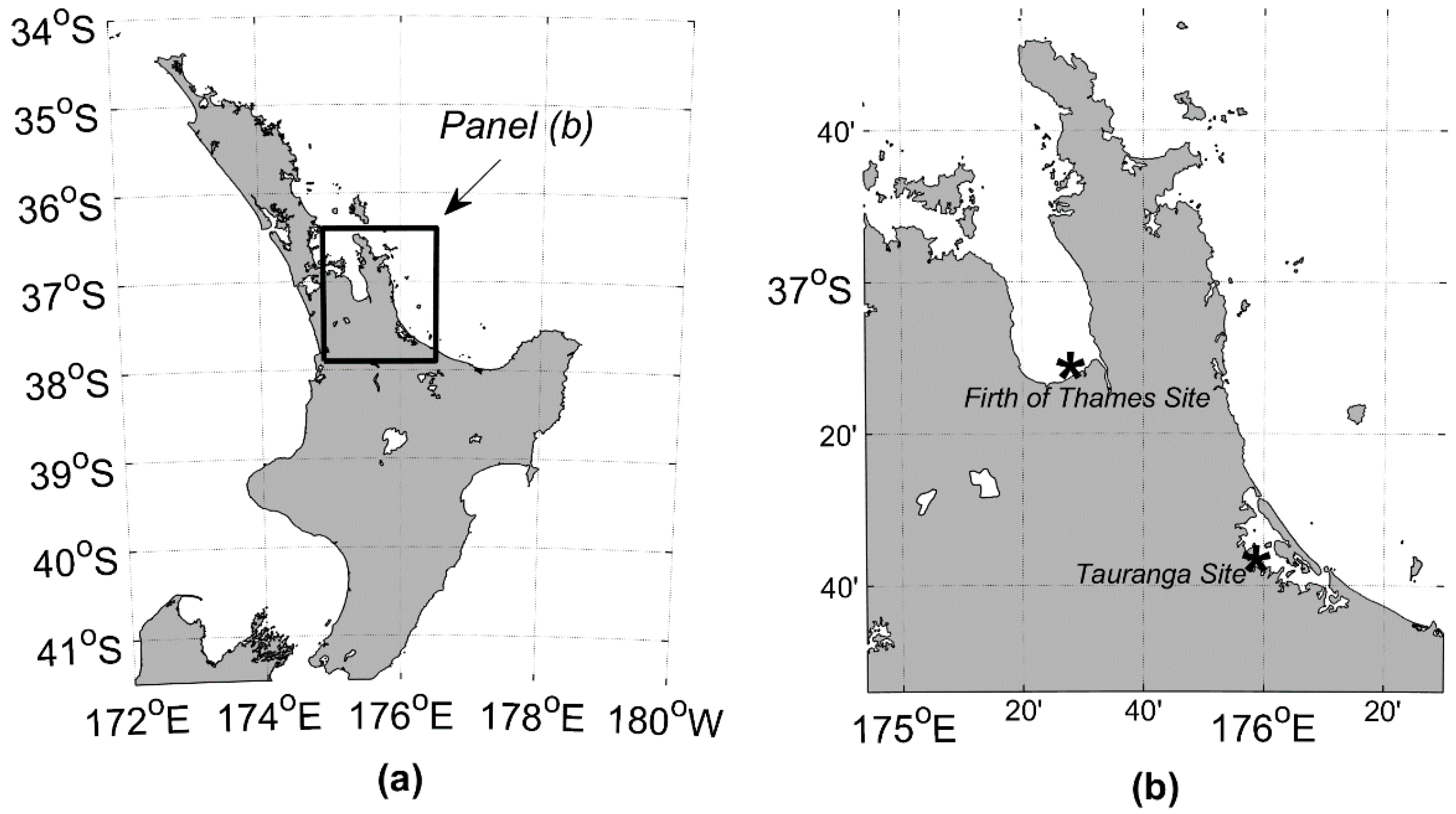
The Firth of Thames (FoT) is a ~800 km2 estuary on New Zealand’s North Island (37°12′ S, 175°27′ E) (Figure 1b). The mesotidal estuary has a spring tidal range of 2.8 m and due to a shallow bed slope and plentiful fine-sediment supply, a large intertidal mudflat has developed [24]. The basin is bounded to the east and west by mountain ranges and the Hauraki Plains to the South. A stopbank (visible as a diagonal track on Figure 2a) prevents the inundation of the Hauraki Plains to the south of the Firth. The basin is exposed to moderate waves from the North and subject to a high terrigenous sediment supply from the Waihou and Piako rivers. The southern boundary of the Firth is colonized by a 1 km wide forest of grey mangroves (Avicennia marina var. australasica).
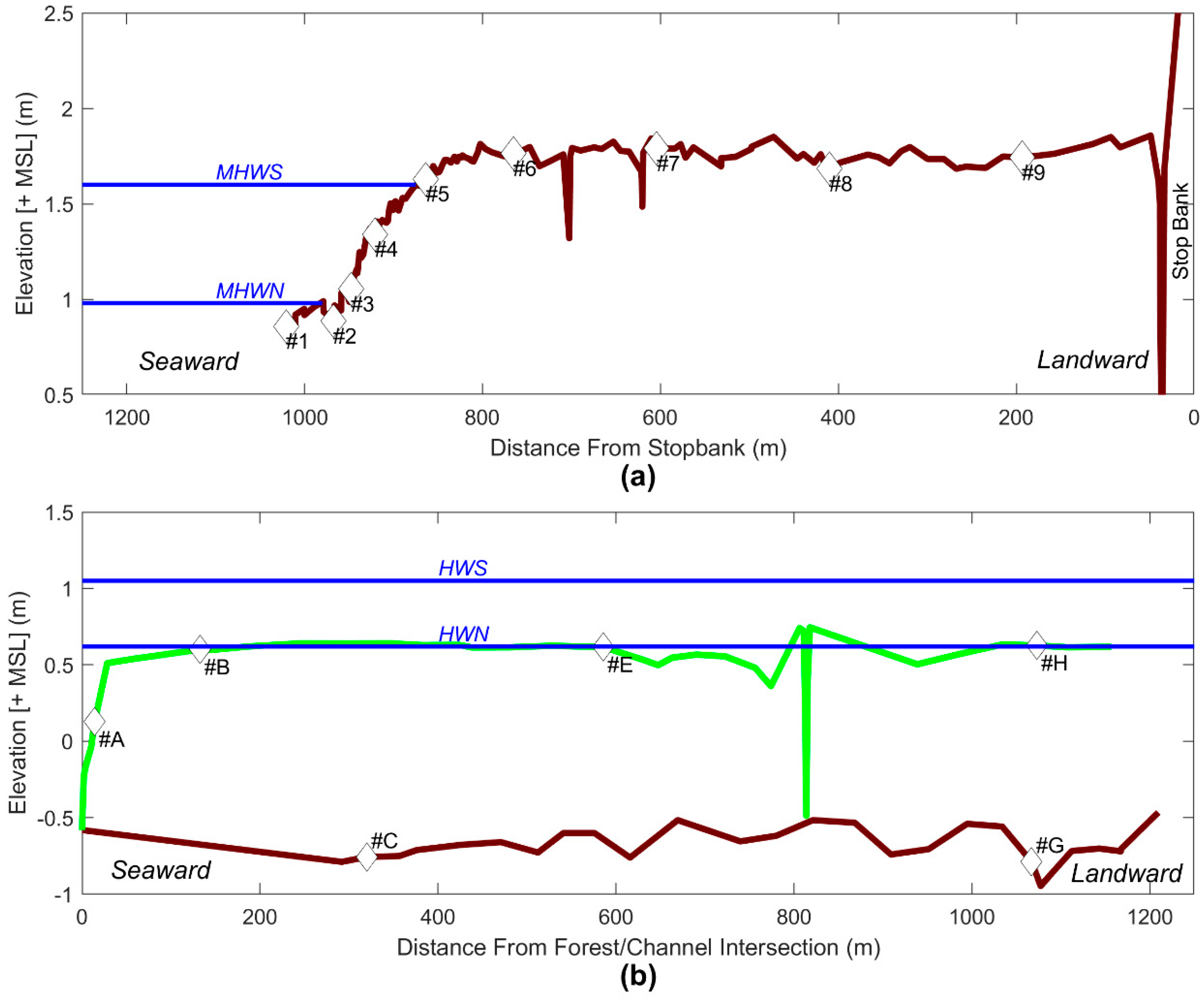
The cross-shore profile of the vegetated region (Figure 3a) consists of a level mangrove forest ~1.7–1.9 m above mean sea level (MSL) extending ~800 m seaward of the stopbank [24]. The sloping vegetation extends an additional ~100 m seaward to the mudflat. The topography and forest characteristics are relatively homogenous in the longshore direction. The elevation of the seaward fringe of the forest is close to a mean high water neap tide level (0.98 m MSL), so the tidal prism within the forest is relatively small and no substantial creeks have developed (Figure 3a) [25].
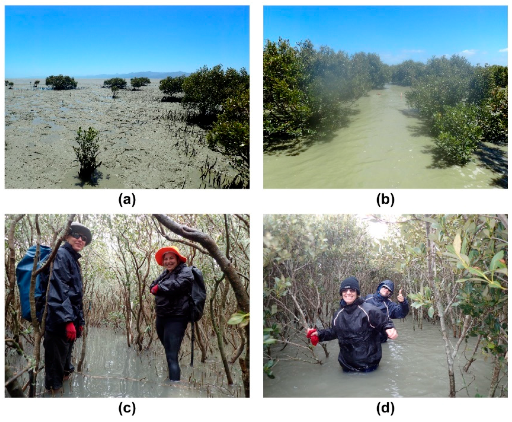
Mangrove characteristics vary throughout the forest. Along the forest fringe, trees are characterized by open spreading forms (Figure 4a,b). Within the forest, trees tend to have straight vertical trunks (Figure 4c). Tree height ranges from 0.5 to 3.5 m. Dense pneumatophores, as many as ~500 m−2, emerge from the bed up to 25 cm in height and ~1 cm in diameter (Table 1).
In November 2016, a supermoon and low-pressure event occurred to produce an unusually large flood event in the Firth of Thames (Figure 4d and Figure 5a,b). The water levels reached 2.36 m above MSL, corresponding to an event with a ~10-year return period for the Firth of Thames. The study area was flooded for several tidal cycles prior to the peak high water and remained flooded for several tidal cycles after the peak water level.
2.1.2. Tauranga Site
Tauranga harbor is a 200 km2 barrier-enclosed lagoon on the North Island of New Zealand (37°39′ S, 176° E) (Figure 1). The mesotidal estuary has an average spring tidal range of 1.62 m and neap range of 1.24 m [26]. Due to the complexity of the estuary, exact tidal ranges are location-dependent [27]. The shallow lagoon, with an average depth of 3 m at low tide, has extensive intertidal areas that make up nearly 2/3 of the estuary area [28]. The estuary has two entrances and is comprised of many sub-estuarine basins. The mangroves in Tauranga have expanded rapidly, from 13 hectares in the 1940s to 168 hectares in 1999 [29]. The mangroves in Tauranga are at the southern boundary of their latitudinal range, which causes the forests to be less productive and the trees to be shorter [23]. The focus of the presented work is a basin north of Pahoia (Figure 1) that nearly drains at low tide.
The Pahoia field site is comprised of a ~1 km long intertidal mangrove forest that occupies ~2/3 of the basin surface area (Figure 2b). Two unvegetated steep-sided channels, along the eastern and western sides of the forest, maintain a near-uniform depth throughout the study site and dominate water flow into the area (Figure 3b and Figure 6b). The western channel bifurcates around a ~300–400 m wide central mangrove platform. The vegetated regions are at the same elevation as high-water neap tidal levels and are approximately flat. A small creek drains into the western channel and further divides the central mangrove forest. The significant tidal prism in the forest is likely responsible for creating the channel network [3].
The forest is comprised of small shrub-like grey mangroves less than 1.2 m in height (average 0.41 m). Individual trees have complex geometry (Figure 7a) and present a low dense canopy (Figure 7b). The pneumatophore density averages 75 per square meter, with individual pencil-roots of similar dimension to the pneumatophores in the Firth of Thames (Table 2).
2.2. Field Data Collection
Field observations were collected during two experiments conducted in November 2016 in the southern Firth of Thames and in April 2017 in the Pahoia sub-estuary of Tauranga Harbor. In each case, arrays of water level sensors were deployed, along with RTK-GPS surveying and manual vegetation surveys. Details of surveys and deployments are given below.
2.2.1. Vegetation Survey
Vegetation surveys were conducted to quantify the rigid vegetation at the study sites. The heterogeneous distribution of vegetation, large study area, and diverse mangrove properties necessitated a unique approach to measure vegetation. The survey objective was targeted at the two types of structure that characterize the flow-reducing properties of Avicennia marina: (1) The pneumatophores and seedling which comprise small, but dense structures near the seabed and (2) the trees and branches which are much less dense but can form a large blocking mechanism at high tide and surge levels. Flexible leafy canopies were not quantified. Mangrove canopies in the Firth of Thames were at sufficient elevation to not submerge and therefore did not influence flow resistance and were not quantified. The shrubby mangroves at Pahoia were submerged at high tide (Figure 7). Attempts were made to quantify canopies in Tauranga using the structure from motion, but were unsuccessful due to the difficulty of gridding the complex leaf geometry. Therefore, the leaves and small branches will provide an unquantified additional blocking. Visual observations indicated that flows were not sufficiently strong to cause the flexing of the leafy vegetation.
Due to the different growth forms of the mangroves at the two sites, slightly different strategies were employed. In the Firth of Thames, mangrove trees in some areas were nearly impenetrable, 5 m by 5 m quadrats were established along the cross-shore instrument transect. In Pahoia, where the mangroves were generally less than a meter tall, a cross-shore and an along-shore transect were established, and vegetation properties measured every 10 m.
In the Firth of Thames, the number of trees was counted in each quadrat. The height and width of the canopy and the stem diameter at 0.3 m from the seabed were manually measured for 5 trees closest to the pre-defined coordinates within the quadrat. To quantify pneumatophores, five 0.5 by 0.5 m quadrats were selected, one at each corner and one at the center of the large quadrat. Within these small quadrats, all the pneumatophores and seedlings were counted. In addition, the height, top diameter, and bottom diameter of five pneumatophores were measured resulting in a total of 25 pneumatophores measured at each station (Table 3).
In Pahoia, a transect through the central mangrove forest was established. Along the transect, the canopy height was measured at 5 m intervals. Pneumatophore and seedling characteristics were measured in 0.5 by 0.5 m quadrats every 5 m using the same method as that used at the Firth of Thames site. Pneumatophore statistics in Table 4 are based on the measurement of 5 pencil roots.
The vegetation drag is estimated as proportional to vegetation frontal area [30]. The frontal area (av) assumes that both the trunks and pneumatophores are rigid emergent vegetation () where n is vegetation element density and d is the average diameter. Note that the contribution of pneumatophores to the total frontal area is reduced when water levels fully submerge the pneumatophores. The direct measurement of trunks in the Firth of Thames was used to generate the frontal area parameter. The complex configuration of plants in Tauranga (Figure 7a) made the measurement of trunks problematic. Therefore, general relationships between trunk density and canopy height, as well as trunk diameter and canopy height, were obtained for the vegetation data in the Firth of Thames. Assuming that the general structural properties of New Zealand Avicennia growth forms are the same between sites, these relationships were used to estimate the trunk density and diameter for Tauranga based on local measured canopy height. This method generates values for frontal area density (with uncertainty because of the assumptions of similarities between sites).
2.2.2. Bathymetry
Manual RTK GPS surveys were conducted to obtain bathymetry at both study sites. In the Firth of Thames, an RTK survey of the instrument transect was conducted using a Trimble R8 GNSS system (Figure 3a). In Tauranga, RTK elevations were obtained for the western channel and a transect through the central mangrove forest (Figure 3b) with a Leica GS18 T GNSS system. Additionally, LIDAR data was provided by local government organizations for both sites (Figure 6). All elevation surveys were initiated and terminated with verification of vertical measurement accuracy with a fixed survey mark, the measurement error never exceeded 3 cm.
2.2.3. Water Level
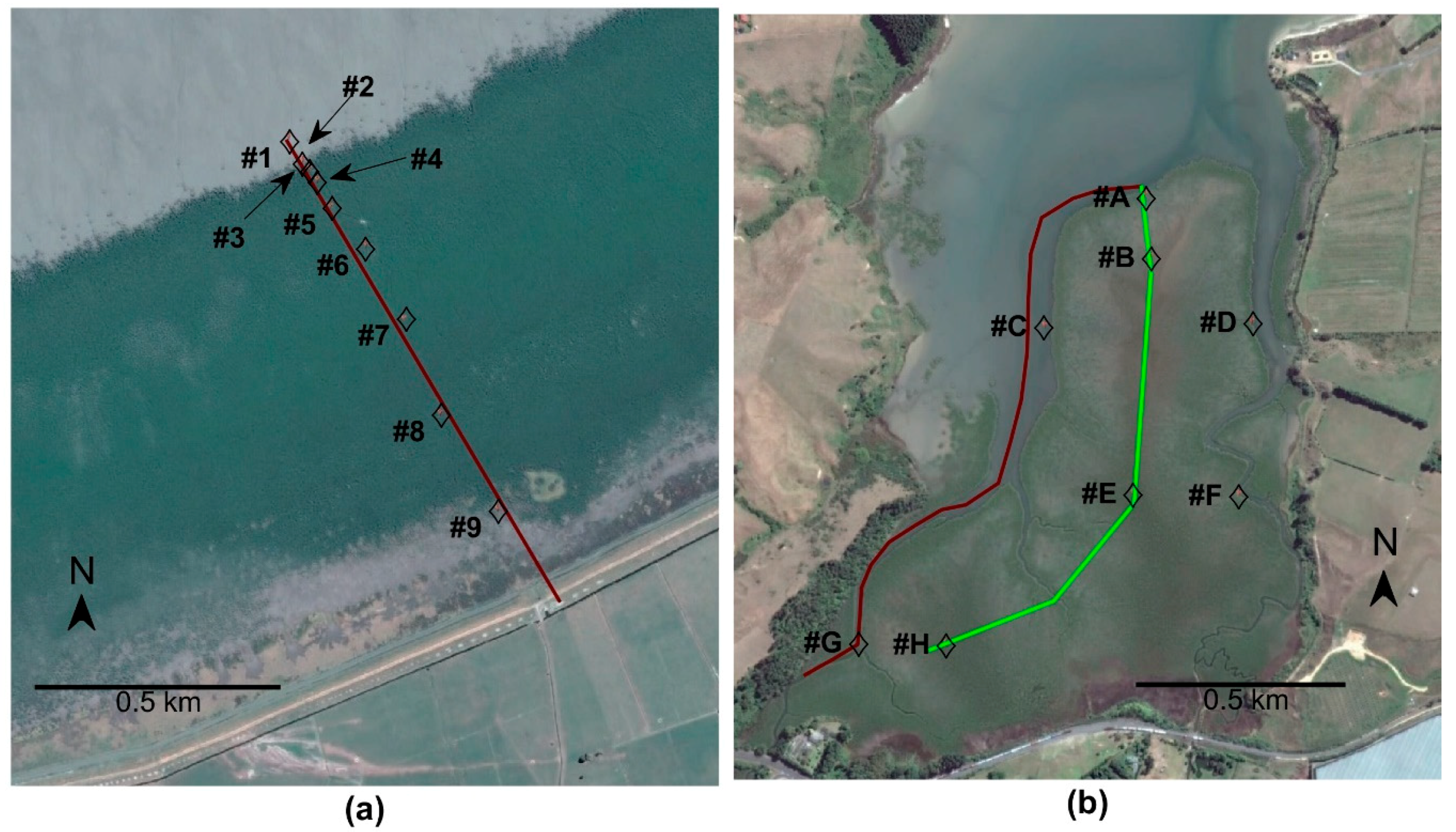
Pressure sensors were deployed at each of the study locations (Figure 2, Table 1 and Table 2). The array of water level sensors deployed in the Firth of Thames in November 2016 consisted of a single transect of 9 instruments, extending from the stopbank to the mudflat (Figure 2a): Station 1 was seaward of the vegetation on the mudflat, stations 2–5 were located across the sloping forest region and stations 6–9 were spread across the forest platform (Figure 3a). A man-made channel is located just seaward of the stopbank and is evident in the transect survey (Figure 3a). At PAHOIA in Tauranga, the central mangrove forest and both the east and west channels were instrumented with pressure gauges (Figure 2b). Station #A is at the seaward edge of the mangroves and at the intersection of the two primary channels. Three stations (#B, #E, and #H) were located at increasing distances into the vegetated intertidal platform. An additional two gauges were positioned in each of the two channels.
Pressure sensors were corrected for variations in barometric pressure and for temperature dependence and referenced to mean sea level using survey data. Pressure signals were smoothed using a low-pass filter and converted to the water level using a constant water density of 1025 kg/m3.
3. Results
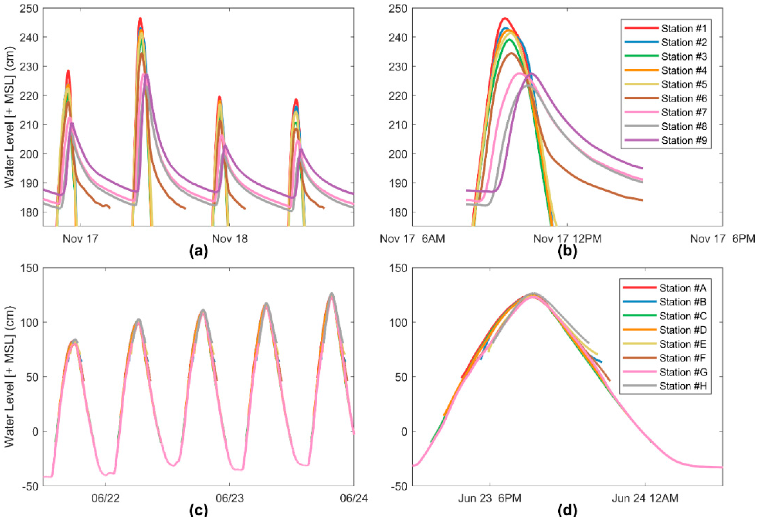
Water levels across the Firth of Thames and Pahoia study sites for successive tidal cycles are displayed in Figure 5. The ~1 km wide mangrove forest in the Firth of Thames site reduced the peak water levels and delayed the inundation signal, with the reduction and delay increasing with distance into the forest. The largest inundation wave in the Firth of Thames reached a maximum of 72 cm above the tidal flat at the seaward forest fringe and decayed to 53 cm above the tidal flat at the landward most station. This water height reduction of 19 cm across the 800 m separation between station 1 and station 9 corresponds to a dissipation rate of ~24 cm/km. The temporal delay in peak water between station 1 and 9 is evident in Figure 5 and estimated at 60 ± 5 min. The average velocity of peak inundation through the Firth of Thames mangrove forest is ~0.2 m/s.
At the Pahoia site, no measurable reduction in water level occurred over the ~1 km separation between instruments. The dissipation of flood levels was less than the uncertainty of the elevation measurements. Additionally, no identifiable temporal delay in peak water occurred over the study site (Figure 5c,d).
The magnitudes of the inundation waves for the two locations are similar with respect to the elevation of the mangrove forest. The inundation waves for both sites range from ~20 to ~70 cm above the average forest elevation (Figure 8). Nonetheless, the elevation of inundation relative to MSL was different between the two sites (Figure 5), with the Firth of Thames ranging from ~220 to ~245 cm above MSL at the seaward boundary of the mangrove forest, while the Tauranga inundation wave varied between 80 and 125 cm above the MSL.
4. Discussion
Mangroves reduce peak water levels during a flood by limiting the exchange of water through the vegetation [18]. Krauss et al. [15] observed that the presence of channels decreased the efficacy of mangrove flood attenuation from 9.4 cm/km to 4.2 cm/km. Using a combination of observations and numerical simulations, Zhang et al. [16] found that the amplitude of storm surge was reduced at a rate of 40–50 cm/km through mangrove forests and ~20 cm/km through patchy regions consisting of a combination of mangrove islands and open water. Flood level reduction during the series of large inundation events in the non-channelized Firth of Thames averaged 24 cm/km, which agrees with rates previously published for unchannelized forests by Krauss et al. and Zhang et al. [15,16]. In contrast, the channelized New Zealand mangrove site in Tauranga had no measurable reduction of flood amplitude. We statistically tested whether tree height and pneumatophore density, diameter and height differed between sites. Because the raw (and transformed) data did not meet the assumptions of normality (Shapiro-Wilk W test p < 0.001) and/or homogeneity of variances (Levene’s test p < 0.01) required for t-tests of differences between means, we used the non-parametric Mann-Whitney U test (a = 0.05). All statistical analyses were conducted in Statistica version 13.2. The results indicated that tree height, pneumatophore density, and pneumatophore height were all significantly different (p < 0.001). As a consequence, the frontal area, and therefore the flow resistance, from trunks was greater in Tauranga than in the Firth of Thames (Table 3 and Table 4). Additionally, Chen et al. [31] demonstrate that mangrove canopies only increase the generation of turbulent kinetic energy by about 10% compared to when the flow is below the bottom of the leaf structures. Despite flow engagement of the dense leafy canopy in Tauranga (Figure 7d), the vegetation had no flood mitigating influence due to preferential routing through the channels.
The interaction of water and vegetation is complex and has been investigated at multiple length scales. At small scales (O (mm)), the boundary layers and shear caused by individual stems, roots, and leaves cause turbulent eddies that shed off each individual stem [32]. Turbulence is also generated at the shear layer between the faster moving flow over submerged vegetation, and the damped flow within the canopy [33]. Intermediate scales (O (m)) comprise flow at the canopy or patch scale involving a community of vegetation. Larger length scale interactions (O (km)) occurs at the forest level [34]. To appropriately investigate a process of interest, a reasonable spatial scale, associated conceptual model, and relevant measurements and methods must be identified [21]. Vegetated regions produce high drag with respect to unvegetated areas and flow is diverted to the path of least resistance. In areas described as dense vegetation patches, most flow is directed around the patches and a forest-wide approach is required. In sparse or homogeneously distributed vegetation, smaller-scale resistance dominates and a smaller-scale approach is justified [35].
In mangrove forests, it is not just the vegetation geometry that controls water transport, the intertidal bathymetry, and water level relative to the elevation of the vegetation also play a role [36,37,38]. Flow through mangrove forests has been categorized into creek flow or sheet flow depending on the primary mechanism of fluid transport. Creek flow dominates in channelized mangroves at low water levels. Sheet flow, the transportation over the vegetated platform through the mangroves, becomes increasingly important with reduced channelization and at increasing water levels [36]. Our results show that the Tauranga mangrove forest is dominated by creek flow, and the density of mangrove vegetation therefore only has minimal contribution to the flow restriction; no evidence of reduced inundation level nor delay in the flood signal exists. In Tauranga, flow resistance is best described by the larger-scale distribution of vegetation and degree of channelization. Conversely, the Firth of Thames mangrove forest is not channelized, and the primary shoreward water transportation mechanism is sheet flow through the vegetation. Here, vegetation properties are important for impeding water exchange across the forest, reducing inundation levels and slowing the flood wave propagation. In the Firth of Thames, the flow resistance relates to the vegetation properties along the one-dimensional cross-shore transect. The cumulative influence of large quantities of individual stems, stalks, and leaves on fluid flows at forest wide scales necessitates simplifying vegetation summary statistics [20]. Several different statistical parameters have been used to describe the influence of vegetation on large-scale flow resistance, including the solid volume fraction, vegetation porosity, and frontal area per bed area [21].
Channelization in mangrove environments develops as the trees grow and create flow resistance and concentrate the flow into channels [3]. However, for initiation of the feedback process that allows the channels to develop, the intertidal platform must be at a sufficiently low elevation with respect to the tidal excursion that currents occur on the vegetated platform. In the case of a very high platform, inundation only occurs at slack water close to high tide, at which time conditions promote sediment deposition. The Tauranga mangrove forest is inundated during normal tidal levels. The drainage channels in the Tauranga study site have likely resulted from scouring by tidally-driven water transport through the forest. The forest elevation in the Firth of Thames is higher than the Mean High Water Spring (MHWS) water levels (Figure 3a) and therefore water is only infrequently transported through the forest and channels cannot develop.
During the study, water depths in the relatively flat mangrove forests in Tauranga and the Firth of Thames were of similar magnitude (Figure 8). The capacity of mangroves to provide coastal flood protection is ultimately related to water transport pathways. Extrapolating from our case study environments, we can expect that lower intertidal areas with channelization will be far less capable of protection than higher intertidal areas with little channelization. Krauss et al. [15] and Zhang et al. (2012) found that the reduction of flood levels along a river corridor was less than through unchannelized vegetation but still provided flood protection. Both previous investigations focused on hurricane-driven storm surges in the south-east United States. The extreme water levels greatly exceeded the capacity of the channel networks, likely resulting in flow pathways through the vegetation and therefore the capacity to mitigate flood levels was apparent but reduced compared to unchannelized locations. Moreover, the sediment regime has been shown to contribute to the development of a profile shape, with muddy profiles often associated with high convex intertidal geometries [39].
5. Conclusions
The influence of mangroves on long wave propagation is strongly dependent on flow routing. In highly channelized mangrove forests, such as our Tauranga case study area, water is preferentially transported via the channels and flood levels are not reduced substantially across the forest. In these cases, the vegetation does not contribute significantly to flow resistance, so specific plant properties are irrelevant with respect to limiting fluid transport. However, we hypothesize that for sufficiently large flood events, in which the conveyance capacity of the channels is exceeded, a proportion of the flow will be forced through the vegetation, which will thus provide an intermediate level of attenuation (still reduced relative to an unchannelized environment). Conversely, in homogeneously vegetated forests without channels, such as the Firth of Thames study site, water is transported through the mangroves and the trees reduce flood levels by limiting fluid exchange through the forest. In these cases, knowledge of vegetation characteristics is essential for the prediction of the rate of flood level reduction.
The degree of channelization and therefore the capacity of mangroves to reduce flooding depends on the elevation of the vegetation. Mangrove forests that occur at relatively low, frequently inundated elevations are subjected to tidal currents that promote channelization, which in turn reduces their capacity to mitigate the flood water level. Higher elevation mangrove forests are inundated only at the peak tide when currents are at a minimum and the sediment regime is depositional. No channel network is created nor maintained, and the capacity of the mangrove forest to reduce flood events is maximized.
Author Contributions
Conceptualization, J.M.M. and K.R.B.; Methodology, J.M.M., K.R.B., E.M.H. and J.C.M.; Formal Analysis, J.M.M.; Data Curation, J.M.M., and E.M.H.; Writing-Original Draft Preparation, J.M.M. & K.R.B.; Writing-Review & Editing, J.M.M., K.R.B., E.M.H. and J.C.M.; Funding Acquisition, K.R.B. and J.C.M.
Funding
This research was funded by the Natural Hazards Platform program (contract C05X0907) AND THE Royal Society Marsden Fund (grant 14-UOW-011).
Acknowledgments
The authors gratefully acknowledge the field help provided by Dean Sandwell, Heide Friedrich, Caitlyn Gillard, Hieu Nguyen, Dave Culliford, and Rex Fairweather. Help with statistical analysis of vegetation was provided by Conrad Pilditch.
Conflicts of Interest
The authors declare no conflict of interest.
References
- Food and Agriculture Organization (FAO). The World’s Mangroves 1980–2005; Food and Agriculture Organization of the United Nations: Rome, Italy, 2007; ISBN 978-92-5-105856-5. [Google Scholar]
- McLeod, E.; Chmura, G.L.; Bouillon, S.; Salm, R.; Bjork, M.; Duarte, C.M.; Lovelock, C.E.; Schlesinger, W.H.; Silliman, B.R. A blueprint for blue carbon: Toward an improved understanding of the role of vegetated coastal habitats in sequestering CO2. Front. Ecol. Environ. 2011, 9, 552–560. [Google Scholar] [CrossRef] [Green Version]
- van Maanen, B.; Coco, G.; Bryan, K.R. On the ecogeomorphological feedbacks that control tidal channel network evolution in a sandy mangrove setting. Proc. R. Soc. A 2015, 471, 20150115. [Google Scholar] [CrossRef] [PubMed] [Green Version]
- Giri, C.; Ochieng, E.; Tieszen, L.L.; Zhu, Z.; Singh, A.; Loveland, T.; Masek, J.; Duke, N. Status and distribution of mangrove forests of the world using earth observation satellite data. Glob. Ecol. Biogeogr. 2011, 20, 154–159. [Google Scholar] [CrossRef]
- Wahl, T.; Haigh, I.D.; Nicholls, R.J.; Arns, A.; Dangendorf, S.; Hinkel, J.; Slangen, A.B.A. Understanding extreme sea levels for broad-scale coastal impact and adaptation analysis. Nat. Commun. 2017, 8, 16075. [Google Scholar] [CrossRef] [PubMed] [Green Version]
- Kroeker, K.J.; Reguero, B.G.; Rittelmeyer, P.; Beckd, M.W. Ecosystem Service and Coastal Engineering Tools for Coastal Protection and Risk Reduction. In Managing Coasts with Natural Solutions; World Bank: Washington, DC, USA, 2016. [Google Scholar]
- Small, C.; Nicholls, R.J. A global analysis of human settlement in coastal zones. J. Coast. Res. 2003, 19, 584–599. [Google Scholar]
- Plant, N.G.; Griggs, G.B. Interactions between nearshore processes and beach morphology near a seawall. J. Coast. Res. 1992, 8, 183–200. [Google Scholar]
- Airoldi, L.; Abbiati, M.; Beck, M.W.; Hawkins, S.J.; Jonsson, P.R.; Martin, D.; Moschellad, P.S.; Sundelofg, A.; Thompsonf, R.C.; Aberg, P. An ecological perspective on the deployment and design of low-crested and other hard coastal defence structures. Coast. Eng. 2005, 52, 1073–1087. [Google Scholar] [CrossRef] [Green Version]
- Guannel, G.; Ruggiero, P.; Faries, J.; Arkema, K.; Pinsky, M.; Gelfenbaum, G.; Guerry, A.; Kim, C.K. Integrated modeling framework to quantify the coastal protection services supplied by vegetation. J. Geophys. Res. Ocean. 2015, 120, 324–345. [Google Scholar] [CrossRef] [Green Version]
- Temmerman, S.; Meire, P.; Bouma, T.J.; Herman, P.; Ysebaert, T.; De Vriend, H.J. Ecosystem-based coastal defence in the face of global change. Nature 2013, 504, 79–83. [Google Scholar] [CrossRef] [PubMed]
- Alongi, D.M. Mangrove forests: Resilience, protection from tsunamis, and responses to global climate change. Estuar. Coast. Shelf Sci. 2008, 76, 1–13. [Google Scholar] [CrossRef]
- Henderson, S.M.; Norris, B.K.; Mullarney, J.C.; Bryan, K.R. Wave-frequency flows within a near-bed vegetation canopy. Cont. Shelf Res. 2017, 147, 91–101. [Google Scholar] [CrossRef]
- Massel, S.; Furukawa, K.; Brinkman, R. Surface wave propagation in mangrove forests. Fluid Dyn. Res. 1999, 24, 219–249. [Google Scholar] [CrossRef]
- Krauss, K.W.; Doyle, T.W.; Doyle, T.J.; Swarzenski, C.M.; From, A.S.; Day, R.H.; Conner, W.H. Water level observations in mangrove swamps during two hurricanes in Florida. Wetlands 2009, 29, 142–149. [Google Scholar] [CrossRef]
- Zhang, K.Q.; Liu, H.Q.; Li, Y.P.; Xu, H.Z.; Shen, J.; Rhome, J.; Smith, T.J. The role of mangroves in attenuating storm surges. Estuar. Coast. Shelf Sci. 2012, 102–103, 11–23. [Google Scholar] [CrossRef]
- U.S. Army Corps of Engineers. Hurricane Study for Morgan City, Louisiana and Vicinity; United States Congress Serial Set: Washington, DC, USA, 1965.
- McIvor, A.; Spencer, T.; Möller, I.; Spalding, M. Storm surge reduction by mangroves. In Natural Coastal Protection Series: Report 2; The Nature Conservancy and Wetlands International: Cambridge, UK, 2012. [Google Scholar]
- Chen, R.; Twilley, R.R. A gap dynamic model of mangrove forest development along gradients of soil salinity and nutrient resources. J. Ecol. 1998, 86, 37–51. [Google Scholar] [CrossRef] [Green Version]
- Mullarney, J.C.; Henderson, S.M. Flows Within Marine Vegetaion Canopies in Advances. In Coastal Hydraulics; Panchange, V., Kaihatu, J., Eds.; World Scientific Publishing: Singapore, 2018; pp. 1–46. [Google Scholar]
- Nepf, H. Hydrodynamics of vegetated channels. J. Hydraul. Res. 2012, 50, 262–279. [Google Scholar] [CrossRef] [Green Version]
- Folkard, A.M. Vegetated flows in their environmental context: A review. Proc. Inst. Civ. Eng.-Eng. Comput. Mech. 2011, 164, 3–24. [Google Scholar] [CrossRef]
- Horstman, E.M.; Lundquist, C.J.; Bryan, K.R.; Bulmer, R.H.; Mullarney, J.C.; Stokes, D.J. The dynamics of expanding mangroves in New Zealand. In Threats to Mangrove Forests; Springer: New York, NY, USA, 2018; pp. 23–51. [Google Scholar] [CrossRef]
- Swales, A.; Bentley, S.J.; Lovelock, C.; Bell, R.G. Sediment processes and mangrove-habitat expansion on a rapidly-prograding muddy coast, New Zealand. In Proceedings of the Coastal Sediments'07, Processing of the Sixth International Symposium on Coastal Engineering and Science of Coastal Sediment Process, New Orleans, LA, USA, 13–17 May 2007. [Google Scholar]
- Swales, A.; Bentley, S.J.; Lovelock, C.E. Mangrove-forest evolution in a sediment-rich estuarine system: Opportunists or agents of geomorphic change? Earth Surf. Proc. Landf. 2015, 40, 1672–1687. [Google Scholar] [CrossRef]
- Heath, R. A review of the physical oceanography of the seas around New Zealand—1982. N. Z. J. Mar. Freshw. Res. 1985, 19, 79–124. [Google Scholar] [CrossRef]
- Tay, H.W.; Bryan, K.R.; de Lange, W.P.; Pilditch, C.A. The hydrodynamics of the southern basin of Tauranga Harbour. N. Z. J. Mar. Freshw. Res. 2013, 47, 249–274. [Google Scholar] [CrossRef] [Green Version]
- Healy, T.R.; Cole, R.; de Lange, W. Geomorphology and ecology of New Zealand shallow estuaries and shorelines. In Estuarine Shores; John Wiley and Sons: New York, NY, USA, 1996. [Google Scholar]
- Park, S.G. Aspects of Mangrove Distribution and Abundance in Tauranga Harbour; Environment Bay of Plenty: Whakatane, New Zealand, 2004.
- Nepf, H. Vegetated flow dynamics. In The Ecogeomorphology of Tidal Marshes; American Geophysical Union: Washington, DC, USA, 2004; pp. 137–163. [Google Scholar]
- Chen, Y.N.; Li, Y.; Cai, T.L.; Thompson, C.; Li, Y. A comparison of biohydrodynamic interaction within mangrove and saltmarsh boundaries. Earth Surf. Proc. Landf. 2016, 41, 1967–1979. [Google Scholar] [CrossRef] [Green Version]
- Norris, B.K.; Mullarney, J.C.; Bryan, K.R.; Henderson, S.M. The effect of pneumatophore density on turbulence: A field study in a Sonneratia-dominated mangrove forest, Vietnam. Cont. Shelf Res. 2017, 147, 114–127. [Google Scholar] [CrossRef]
- Horstman, E.; Bryan, K.; Mullarney, J.; Pilditch, C.; Eager, C. Are flow-vegetation interactions well represented by mimics? A case study of mangrove pneumatophores. Adv. Water Resour. 2018, 111, 360–371. [Google Scholar] [CrossRef]
- Mullarney, J.C.; Henderson, S.M.; Reyns, J.A.; Norris, B.K.; Bryan, K.R. Spatially varying drag within a wave-exposed mangrove forest and on the adjacent tidal flat. Cont. Shelf Res. 2017, 147, 102–113. [Google Scholar] [CrossRef]
- Green, J.C. Comparison of blockage factors in modelling the resistance of channels containing submerged macrophytes. River Res. Appl. 2005, 21, 671–686. [Google Scholar] [CrossRef]
- Horstman, E.M.; Dohmen-Janssen, C.M.; Bouma, T.J.; Hulscher, S.J.M.H. Tidal-scale flow routing and sedimentation in mangrove forests: Combining field data and numerical modelling. Geomorphology 2015, 228, 244–262. [Google Scholar] [CrossRef]
- Mazda, Y.; Kanazawa, N.; Wolanski, E. Tidal asymmetry in mangrove creeks. Hydrobiologia 1995, 295, 51–58. [Google Scholar] [CrossRef]
- Mei, C.C.; Chan, I.C.; Liu, P.L.F.; Huang, Z.; Zhang, W. Long waves through emergent coastal vegetation. J. Fluid Mech. 2011, 687, 461–491. [Google Scholar] [CrossRef]
- Bryan, K.R.; Nardin, W.; Mullarney, J.C.; Fagherazzi, S. The role of cross-shore tidal dynamics in controlling intertidal sediment exchange in mangroves in Cù Lao Dung, Vietnam. Cont. Shelf Res. 2017, 147, 128–143. [Google Scholar] [CrossRef]
Figure 1.
(a) The North Island of New Zealand with a panel (b) outlined; (b) Section of North Island of New Zealand showing the proximity of the Firth of Thames and Tauranga mangrove sites.
Figure 1.
(a) The North Island of New Zealand with a panel (b) outlined; (b) Section of North Island of New Zealand showing the proximity of the Firth of Thames and Tauranga mangrove sites.

Figure 2.
(a) The Firth of Thames study site with 9 (#1 seaward–#9 landward) instrument locations noted and bathymetry survey transect (brown). Station #1 is on the unvegetated mudflat, station #2 is in the vegetation fringe, stations #3–#5 are in the gently sloping intertidal, and stations #6–#9 are on the intertidal flat; (b) The Tauranga study site with 8 instrument locations noted with channel thalweg bathymetry survey (brown) and central mangrove survey (green). Station #A is on the vegetation fringe on the seaward boundary, stations #C and #D are in the western channel, stations #B, #E, and #H are in the central mangrove forest, stations #D and #F are in the eastern channel.

Figure 3.
(a) The elevation profile along the instrument transect in the Firth of Thames. Mean High Water Spring (MHWS) and Mean High Water Neap (MHWN) are noted. The main forest is higher than normal tidal levels and therefore no drainage channels have been scoured by tidal water flow; (b) the Tauranga RTK survey of transect through central mangrove forest (green) and thalweg (brown). High Water Spring (HWS) and High Water Neap (HWN) are marked (blue). The semi-diurnal tidally-driven flow through the forest is responsible for channelization at the site.

Figure 4.
The images of Firth of the Thames study site. (a) Forest fringe at low tide; (b) Fringe at mid tide, trees are characterized with open spreading branches; (c) Interior mangrove forest with two researchers for scale. Trees are tall with vertical trunks; (d) Two researchers in the mangrove forest during the flood event.

Figure 5.
(a) The Firth of Thames water level at each instrument station for five consecutive spring tidal cycles. The upper intertidal flat (stations #6–#9) did not fully drain for several tidal cycles; (b) Firth of Thames water level during maximum inundation event; (c) Tauranga water level for five consecutive spring tidal cycles. Note that only station #G was submerged at low tide; (d) Tauranga water level during the largest tidal cycle.

Figure 6.
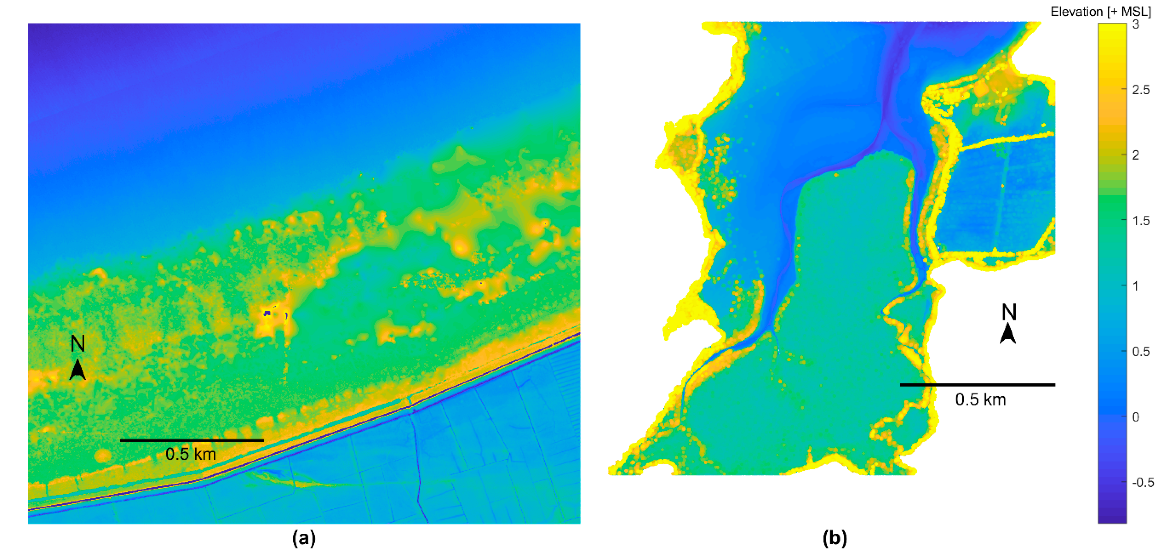
(a) The Firth of Thames LiDAR devoid of a channel network. Patchy higher elevations likely indicate a vegetation canopy; (b) Tauranga LiDAR data. Deep, incised channels and a level vegetated intertidal characterize the site. High elevation along channels displays a dense mangrove canopy. The color bar shows an elevation scale for both subplots.
Figure 6.
(a) The Firth of Thames LiDAR devoid of a channel network. Patchy higher elevations likely indicate a vegetation canopy; (b) Tauranga LiDAR data. Deep, incised channels and a level vegetated intertidal characterize the site. High elevation along channels displays a dense mangrove canopy. The color bar shows an elevation scale for both subplots.

Figure 7.
The images of the Tauranga study site. (a) Example mangrove tree. Vegetation is characterized by a complex trunk structure and a low canopy height; (b) Mangrove forest at mid tide; (c) Mangrove lined channel with steep densely vegetated banks; (d) Weather station recording barometric pressure and wind speed during high spring tide with canopy almost submerged.

Figure 8.
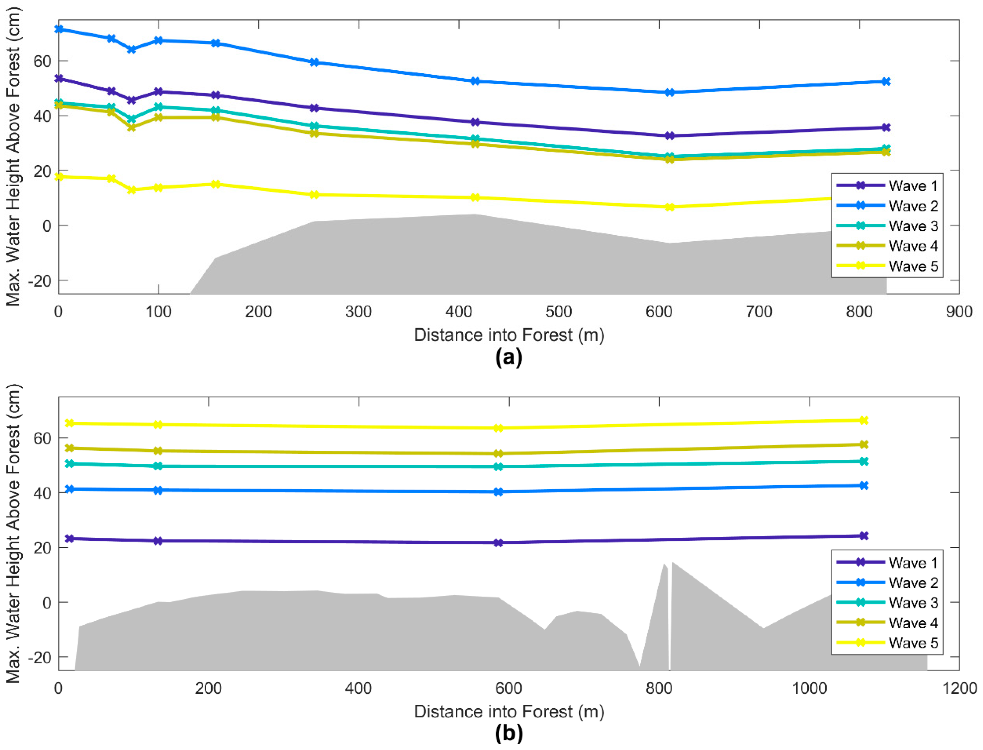
(a) The peak water level at each instrument station along the transect in the Firth of Thames for 5 consecutive inundation events; (b) the peak water level at each instrument along the central mangrove transect in Tauranga (#A, #B, #E, and #H). Elevations are with respect to average elevation of the forest floor, profiles of which are shown in grey.
Figure 8.
(a) The peak water level at each instrument station along the transect in the Firth of Thames for 5 consecutive inundation events; (b) the peak water level at each instrument along the central mangrove transect in Tauranga (#A, #B, #E, and #H). Elevations are with respect to average elevation of the forest floor, profiles of which are shown in grey.


Table 1.
The Firth of Thames instrument array. Note that during factory calibration, the Aquadopp depth uncertainty over the range of interest was <5 cm and the Vector uncertainty was <2 cm.
Table 1.
The Firth of Thames instrument array. Note that during factory calibration, the Aquadopp depth uncertainty over the range of interest was <5 cm and the Vector uncertainty was <2 cm.
| Station | Instrument | Sampling | Temperature Dependence | Depth Measurement Uncertainty | |
|---|---|---|---|---|---|
| Regime | Details | Correction Applied | (cm) | ||
| #1 | Nortek Aquadopp | Burst | 212 samples at 8 Hz every 15 min | Y | <10 |
| #2 | Nortek Vector | Burst | 7.5 min sampling at 16 Hz every 15 min | Y | <5 |
| #3 | Nortek Aquadopp | Burst | 212 samples at 8 Hz every 15 min | Y | <10 |
| #4 | Nortek Aquadopp | Burst | 212 samples at 8 Hz every 15 min | Y | <10 |
| #5 | RBR Concerto | Continuous | 4 Hz | N | <1 |
| #6 | RBR Duet | Continuous | 8 Hz | N | <1 |
| #7 | Solinst Levelogger | Continuous | 1/60 Hz | N | <1 |
| #8 | Solinst Levelogger | Continuous | 1/60 Hz | N | <1 |
| #9 | Solinst Levelogger | Continuous | 1/60 Hz | N | <1 |
| Weather Station | Continuous | 1/5 min | N | <1 | |
Table 2.
The Tauranga instrument array.
| Station | Instrument | Sampling | Temperature Dependence | Depth Measurement Uncertainty | |
|---|---|---|---|---|---|
| Regime | Details | Correction Applied | (cm) | ||
| #A | RBR Solo | Continuous | 8 Hz | N | <1 |
| #B | RBR Solo | Continuous | Every 2 min Average 1 min of data sampled at 4 Hz | N | <1 |
| #C | RBR Duet | Continuous | 8 Hz | N | <1 |
| #D | RBR Duet | Continuous | 8 Hz | N | <1 |
| #E | RBR Solo | Continuous | Every 2 min Average 1 min of data sampled at 4 Hz | N | <1 |
| #F | RBR Solo | Continuous | 8 Hz | N | <1 |
| #G | RBR Solo | Continuous | 8 Hz | N | <1 |
| #H | RBR Solo | Continuous | 8 Hz | N | <1 |
| Weather Station | Continuous | 1/5 min | N | <1 | |
Table 3.
The Firth of Thames vegetation survey summary. The values given are averages with the standard deviation where appropriate.
Table 3.
The Firth of Thames vegetation survey summary. The values given are averages with the standard deviation where appropriate.
| Location | Trees | Pneumatophores | |||||||
|---|---|---|---|---|---|---|---|---|---|
| Description | Distance from Fringe | Density | Height | Diameter | Frontal Area | Density | Height | Diameter | Frontal Area |
| (m) | (# per m2) | (m) | (cm) | (m−1) | (# per m2) | (cm) | (cm) | (m−1) | |
| Mudflat | −49 | 0.1 | 0.6 | 1.6 | 0.00 | 0 | 0 | 0 | 0 |
| Fringe (Front) | 0 | 0.1 | 2.3 | 6.4 | 0.01 | 126 | 25.4 (8.5) | 0.6 (0.2) | 0.76 |
| Fringe (Back) | 22 | 1.0 | 1.9 (1.1) | 4.8 (5.4) | 0.05 | 385 | 22.9 (9.1) | 0.6 (0.2) | 2.31 |
| Forest | 36 | 1.0 | 2.9 (0.3) | 5.8 (3.1) | 0.06 | 386 | 17.0 (6.9) | 0.5 (0.2) | 1.93 |
| Forest | 114 | 6.4 | 2.3 (0.2) | 3.0 (0.7) | 0.19 | 322 | 12.5 (5.6) | 0.6 (0.2) | 1.93 |
| Forest | 166 | 11.4 | 1.5 (0.3) | 2.8 (1.2) | 0.32 | 357 | 7.7 (4.4) | 0.6 (0.2) | 2.14 |
| Forest | 262 | 12.2 | 1.2 (0.1) | 1.9 (0.4) | 0.23 | 481 | 8.3 (4.1) | 0.6 (0.1) | 2.89 |
| Forest | 376 | 6.4 | 3.1 (0.1) | 3.6 (1.1) | 0.23 | 342 | 8.7 (5.4) | 0.5 (0.1) | 1.71 |
| Forest | 476 | 1.4 | 3.8 (0.3) | 4.2 (1.1) | 0.06 | 330 | 10.5 (5.5) | 0.6 (0.1) | 1.98 |
| Forest | 561 | 3.6 | 1.6 (0.2) | 3.9 (2.2) | 0.14 | 570 | 12.0 (6.1) | 0.5 (0.1) | 2.85 |
| Forest | 667 | 5 | 2.6 (0.3) | 3.8 (0.6) | 0.19 | 482 | 11.0 (4.7) | 0.5 (0.1) | 2.41 |
Table 4.
The Tauranga vegetation survey summary. The values given are averages with the standard deviation where appropriate.
Table 4.
The Tauranga vegetation survey summary. The values given are averages with the standard deviation where appropriate.
| Location | Trees | Pneumatophores | |||||
|---|---|---|---|---|---|---|---|
| Transect | Distance from Fringe | Canopy Height | Frontal Area * | Density | Height | Diameter | Frontal Area |
| (m) | (m) | (m−1) | (# per m2) | (cm) | (cm) | (m−1) | |
| Along-shore | 0 | 0 | 0.26 | 40 | 1.5 (0.5) | 0.3 (0.2) | 0.12 |
| Along-shore | 5 | 0.97 | 0.26 | 164 | 1.7 (0.5) | 0.3 (0.2) | 0.49 |
| Along-shore | 15 | 0.48 | 0.26 | 296 | 1.1 (0.4) | 0.4 (0.2) | 1.18 |
| Along-shore | 25 | 0.41 | 0.26 | 308 | 1.1 (0.5) | 0.5 (0.2) | 1.54 |
| Along-shore | 35 | 0.36 | 0.26 | 296 | 0.6 (0.5) | 0.4 (0.2) | 1.18 |
| Along-shore | 45 | 0.38 | 0.26 | 252 | 1 (0.6) | 0.4 (0.2) | 1.00 |
| Along-shore | 55 | 0.365 | 0.26 | 248 | 6 (3.7) | 0.5 (0.2) | 1.24 |
| Along-shore | 65 | 0.34 | 0.26 | 356 | 8.7 (4.2) | 0.6 (0.1) | 2.14 |
| Along-shore | 75 | 0.37 | 0.26 | 196 | 10.8 (2.8) | 0.6 (0.2) | 1.18 |
| Along-shore | 85 | 0.29 | 0.25 | 244 | 7 (2.6) | 0.6 (0.1) | 1.46 |
| Along-shore | 95 | 0.23 | 0.26 | 240 | 5.1 (2.4) | 0.6 (0.1) | 1.44 |
| Along-shore | 105 | 0.26 | 0.26 | 216 | 10.3 (4.1) | 0.5 (0.2) | 1.08 |
| Along-shore | 115 | 0.27 | 0.25 | 172 | 4.3 (1.8) | 0.6 (0.2) | 1.03 |
| Along-shore | 125 | 0.22 | 0.26 | 172 | 5.3 (3.2) | 0.5 (0.2) | 0.86 |
| Along-shore | 135 | 0.29 | 0.26 | 264 | 6.9 (3.6) | 0.5 (0.1) | 1.32 |
| Along-shore | 145 | 0.26 | 0.25 | 248 | 7.4 (3.5) | 0.5 (0.2) | 1.24 |
| Along-shore | 155 | 0.23 | 0.25 | 364 | 6.3 (3.7) | 0.6 (0.2) | 2.18 |
| Along-shore | 165 | 0.23 | 0.25 | 292 | 6.1 (3.3) | 0.6 (0.2) | 1.75 |
| Along-shore | 175 | 0.22 | 0.25 | 252 | 6.2 (2.1) | 0.7 (0.2) | 1.76 |
| Along-shore | 185 | 0.2 | 0.25 | 172 | 6.3 (2.5) | 0.7 (0.1) | 1.20 |
| Along-shore | 195 | 0.2 | 0.26 | 200 | 13.6 (7.1) | 0.6 (0.2) | 1.20 |
| Along-shore | 205 | 0.32 | 0.26 | 212 | 5.4 (3.1) | 0.5 (0.1) | 1.06 |
| Along-shore | 215 | 0.3 | 0.26 | 224 | 11.2 (2.9) | 0.6 (0.1) | 1.34 |
| Along-shore | 225 | 0.24 | 0.26 | 192 | 7 (6.0) | 0.5 (0.1) | 0.96 |
| Along-shore | 200 | 0.27 | 0.26 | 276 | 11.7 (2.8) | 0.6 (0.2) | 1.66 |
| Along-shore | 190 | 0.29 | 0.26 | 324 | 3.7 (2.5) | 0.6 (0.2) | 1.94 |
| Cross-shore | 180 | 0.33 | 0.26 | 344 | 8.2 (6.3) | 0.6 (0.2) | 2.06 |
| Cross-shore | 170 | 0.52 | 0.26 | 192 | 11.7 (8.0) | 0.6 (0.1) | 1.15 |
| Cross-shore | 160 | 0.36 | 0.26 | 340 | 14.2 (7.1) | 0.6 (0.1) | 2.04 |
| Cross-shore | 150 | 0.35 | 0.26 | 356 | 8.5 (5.2) | 0.6 (0.1) | 2.14 |
| Cross-shore | 140 | 0.47 | 0.26 | 348 | 12.9 (7.3) | 0.6 (0.2) | 2.09 |
| Cross-shore | 130 | 0.54 | 0.26 | 396 | 10.2 (3.9) | 0.6 (0.2) | 2.38 |
| Cross-shore | 110 | 0.59 | 0.26 | 404 | 15.1 (7.0) | 0.6 (0.2) | 2.42 |
| Cross-shore | 100 | 0.63 | 0.26 | 536 | 12.7 (4.3) | 0.6 (0.1) | 3.22 |
| Cross-shore | 90 | 0.64 | 0.26 | 400 | 10.7 (2.5) | 0.5 (0.1) | 2.00 |
| Cross-shore | 80 | 0.71 | 0.26 | 552 | 8.1 (4.0) | 0.5 (0.1) | 2.76 |
| Cross-shore | 70 | 0.93 | 0.26 | 568 | 7.4 (2.7) | 0.5 (0.1) | 2.84 |
| Cross-shore | 60 | 0.55 | 0.26 | 404 | 8.8 (4.1) | 0.6 (0.2) | 2.42 |
| Cross-shore | 50 | 0.56 | 0.26 | 464 | 15.9 (8.6) | 0.6 (0.1) | 2.78 |
| Cross-shore | 40 | 0.42 | 0.26 | 408 | 7.6 (6.1) | 0.5 (0.1) | 2.04 |
| Cross-shore | 30 | 0.44 | 0.26 | 444 | 8.9 (4.2) | 0.6 (0.1) | 2.66 |
| Cross-shore | 20 | 0.72 | 0.25 | 308 | 10.5 (5.0) | 0.5 (0.1) | 1.54 |
| Cross-shore | 10 | 1.3 | 0.26 | 432 | 5.4 (2.8) | 0.5 (0.1) | 2.16 |
| Cross-shore | 0 | 0.97 | 0.26 | 268 | 12.8 (5.3) | 0.5 (0.1) | 1.34 |
* Note that tree stem diameter and density for frontal area density calculation has been estimated (see text for details).
© 2018 by the authors. Licensee MDPI, Basel, Switzerland. This article is an open access article distributed under the terms and conditions of the Creative Commons Attribution (CC BY) license (http://creativecommons.org/licenses/by/4.0/).
Share and Cite
MDPI and ACS Style
Montgomery, J.M.; Bryan, K.R.; Horstman, E.M.; Mullarney, J.C. Attenuation of Tides and Surges by Mangroves: Contrasting Case Studies from New Zealand. Water 2018, 10, 1119. https://doi.org/10.3390/w10091119
AMA Style
Montgomery JM, Bryan KR, Horstman EM, Mullarney JC. Attenuation of Tides and Surges by Mangroves: Contrasting Case Studies from New Zealand. Water. 2018; 10(9):1119. https://doi.org/10.3390/w10091119
Chicago/Turabian StyleMontgomery, John M., Karin R. Bryan, Erik M. Horstman, and Julia C. Mullarney. 2018. "Attenuation of Tides and Surges by Mangroves: Contrasting Case Studies from New Zealand" Water 10, no. 9: 1119. https://doi.org/10.3390/w10091119
Note that from the first issue of 2016, this journal uses article numbers instead of page numbers. See further details here.