Evaluation of Potential Evapotranspiration Based on CMADS Reanalysis Dataset over China

Abstract

Potential evapotranspiration (PET) is used in many hydrological models to estimate actual evapotranspiration. The calculation of PET by the Food and Agriculture Organization of the United Nations (FAO) Penman–Monteith method requires data for several meteorological variables that are often unavailable in remote areas. The China Meteorological Assimilation Driving Datasets for the SWAT model (CMADS) reanalysis datasets provide an alternative to the use of observed data. This study evaluates the use of CMADS reanalysis datasets in estimating PET across China by the Penman–Monteith equation. PET estimates from CMADS data (PET_cma) during the period 2008–2016 were compared with those from observed data (PET_obs) from 836 weather stations in China. Results show that despite PET_cma overestimating average annual PET and average seasonal in some areas (in comparison to PET_obs), PET_cma well matches PET_obs overall. Overestimation of average annual PET occurs mainly for western inland China. There are more meteorological stations in southeastern China for which PET_cma is a large overestimate, with percentage bias ranging from 15% to 25% for spring but a larger overestimate in the south and underestimate in the north for the winter. Wind speed and solar radiation are the climate variables that contribute most to the error in PET_cma. Wind speed causes PET to be underestimated with percentage bias in the range −15% to −5% for central and western China whereas solar radiation causes PET to be overestimated with percentage bias in the range 15% to 30%. The underestimation of PET due to wind speed is offset by the overestimation due to solar radiation, resulting in a lower overestimation overall.

1. Introduction

Evapotranspiration (ET) is a fundamental component of the hydrological cycle and a route for energy transfer between the earth’s surface and the atmosphere. It is important in activities such as evaluating water resources [1], drought forecasting [2], and managing irrigation [3]. It is also important for an understanding of the behavior of water in soil–vegetation–atmosphere interactions [4] and in rainfall-runoff modeling.

Actual evapotranspiration is usually measured indirectly by eddy covariance (EC) [5], the Bowen ratio method [6], lysimetry [7], and scintillometry [8]; ET cannot be observed at a large scale by these techniques. Eddy towers and the Bowen ratio method observe over only hundreds of meters, depending on wind speed, tower height, and canopy level. The lysimeter only functions on a scale of several meters. The scintillometer measures sensible heat flux on the scale of kilometers [9]. Wang and Dickinson [10] review these observation methods and summarize different methods of modeling ET. For studies on a catchment, regional, or global scale, ET can be estimated by remote sensing methods [11], hydrological models, and land surface models [12,13]. The use of remote sensing methods may be restricted by a relatively low temporal resolution, and some remote sensing methods are only suitable in the clear sky condition [11]. Hydrological models and land surface models can estimate ET for different spatial and temporal scales, which makes them able to support the management and planning of water resources better than other techniques.

Potential evapotranspiration (PET) has been used in many hydrological models to estimate actual evapotranspiration using a soil moisture extraction function [14]. PET is defined as the amount of water that can potentially be removed from a vegetated surface through the processes of evaporation or transpiration with no forcing other than atmospheric demand [15]. The common methods of estimating PET can be divided into four categories: radiation-based, temperature-based, a combination of these two, and mass transfer [16,17]. These methods differ in their input requirements and their underlying assumptions. Some are developed for a specific climatic region [18]. The Penman–Monteith equation has been incorporated in many hydrological models, such as SWAT [19], VIC [20], and SHE [21], to estimate PET. Many studies have compared different PET estimation methods [18,22]. Kite and Drooger [23] evaluated eight different methods and found the Food and Agriculture Organization of the United Nations Penman–Monteith method (FAO-PM), which combines mass transfer and energy balance with temperature and vegetation conductance, best models PET, and most closely matches field observations. FAO-PM requires observed maximum temperature, minimum temperature, air temperature, wind speed, relative humidity, and solar radiation (or solar duration) as input variables. In China, meteorological stations are not evenly distributed spatially, and observed records of these climate variables are difficult to obtain in some rural areas. Reanalysis datasets, which have high precision and high spatiotemporal resolution, complement this data paucity and they have been extensively used in hydrological modeling.

There are many widely used reanalysis products, which include climate forecast system reanalysis (CFSR) [24], NCEP/DOE [25] and NCEP/NCAR [26] from NCEP, ERA-15 [27], ERA40 [28] and ERA-Interim [29] from ECMWF, JRA-55 from the Japanese meteorological agency [30], and MERRA from NASA [31]. They have provided accurate meteorological data and have shown they can overcome the disadvantages of thinly distributed observation networks. There have been extensive evaluations of the performance of these reanalysis products over different regions of the world [32,33,34]. PET estimates derived from reanalysis products have been compared. Weiland et al. used CFSR and compared global PET estimates from six different methods [35]. Srivastava et al. evaluated PET calculated from NCEP and ECMWF ERA-Interim data in England [36]. Trambauer et al. compared observed evaporation for Africa using a continental version of the global hydrological model PCR-GLOBWB with PET estimates given by the ECMWF reanalysis products ERA-Interim and ERA-Land, and satellite-based products MOD16 and GLEAM [37]. These products provide global climate datasets having a relatively coarse spatial resolution.

The newly developed China Meteorological Assimilation Driving Datasets for the SWAT model (CMADS) covers East Asia (60°–160° E, 0°–65° N). CMADS was developed to provide meteorological data with fine resolution. Temperature, pressure, and wind speed data were derived from hourly observations from 2421 national weather stations and 29,452 regional weather stations. The data were combined using the Space and Time Multiscale Analysis System (STMAS) with European Centre for Medium-Range Weather Forecasts (ECMWF) ambient field. Precipitation data were incorporated by combining observed data from weather stations with precipitation reanalysis data from the NOAA with CPC MORPHing technique (CMORPH). Solar radiation data obtained from radiance data of the International Satellite Cloud Climatology Project (ISCCP) were combined with data retrieved from the FY-2E satellite using the discrete-ordinate radiative transfer (DISTORT) model. Big data projection and processing methods, such as loop nesting of data, projection of resampling models, and bilinear interpolation, were used to build the datasets [38,39,40]. There have been many similar applications in different river basins in East Asia that have achieved satisfactory results in rainfall–runoff simulation [41,42,43,44,45,46,47,48,49].

The objectives of this study are: (1) to evaluate the accuracy of PET estimated by the Penman-Monteith equation (PM) using CMADS reanalysis data by comparing it with PET estimated by PM using observed data provided by 836 weather stations; (2) to analyze the contribution of each reanalysis variable from the CMADS data to error in PET by controlling the variables. Several statistical measures were chosen to evaluate the comparison between CMADS-derived PET and observed PET.

2. Materials and Methods

2.1. Data and Study Area

Meteorological data for maximum temperature, minimum temperature, wind speed at 10 m height, relative humidity, and solar duration from 836 weather stations were collected to estimate PET. The spatial distribution of the 836 weather stations across China is shown in Figure 1. PM is one of the most widely used methods of calculating PET [50,51,52,53,54]. Details of estimating PET using PM are given in the following paragraph. In the rest of this paper, PET values derived from the weather station observations are referred to as PET_obs. They are taken to be the real values against which other predicted PET values can be compared.

PET over China was also estimated using CMADS (version 1.1). The CMADS dataset spans the period 2008–2016 at a spatial resolution of 0.25°; it covers East Asia (60°–160° E, 0°–65° N) and provides daily data for the meteorological variables. The datasets were developed by Xianyong Meng and are available from the website: http://www.cmads.org. In this study, we used daily maximum temperature (T_max), daily minimum temperature (T_min), relative humidity (RH), solar radiation (Rs), and wind speed at 10m height (u₁₀) to estimate PET using PM. PET values derived from the CMADS datasets (PET_cma) were compared with PET_obs values and differences are referred to as under or overestimation (PET_cma < PET_obs or PET_cma > PET_obs).

Because the gridded CMADS data observations do not spatially correspond to the weather station observations, the CMADS grids were interpolated to the 836 stations using a polynomial interpolation method. Temperature differences caused by elevation are also considered in the interpolation: temperature was assumed to decrease by 0.65 °C for every 100 m increase in elevation.

2.2. Penman–Monteith Equation for Potential Evapotranspiration

The Food and Agriculture Organization (FAO) Expert Consultation of Revision of FAO Methodologies of Crop Water Requirements standardized the types and characteristics of the vegetated surface based on the previous PET definition. The definition of vegetated surface was assumed to be a hypothetical reference crop with a crop height of 0.12 m, a fixed surface resistance of 70 s m⁻¹ and albedo of 0.23 [50]. The daily potential evapotranspiration (PET, mm/day) estimated by the Penman–Monteith equation (PM) is:

$$\mathrm{PET}=\frac{0.408\Delta \left(R_n-G \right)+\gamma \frac{900}{T_{mean}+273.3}{u}_2\left(e_s-e_a\right)}{\Delta +\gamma \left(1+0.34\right)u_2}$$

(1)

where: R_n is the net radiation at the crop surface (MJ m⁻² day⁻¹); G is the soil heat flux density (MJ m⁻² day⁻¹), which is assumed to be zero as the magnitude of G, in this case, is relatively small; T_mean is the mean daily air temperature (°C); u₂ is the wind speed at 2 m height (m s⁻¹); e_s is the saturation vapor pressure (kPa); e_a is the actual vapor pressure (kPa); e_s − e_a is the vapor pressure deficit (kPa); Δ is the slope of the relationship between saturation vapor pressure and mean daily air temperature (kPa °C⁻¹); γ is the psychrometric constant which depends on the altitude of each location (kPa °C⁻¹).

Saturation vapor pressure is related to air temperature and can be calculated from air temperature. The relationship is expressed in Equation (2), in which: e_s is the mean of the saturation vapor pressure at T_max and T_min; e_a was calculated by multiplying the average values of the saturation vapor pressure at T_max and T_min by the mean daily relative humidity. The FAO recommendation is to calculate the actual vapor pressure by taking the average the product of vapor pressure at the higher temperature and daily low humidity and the product of vapor pressure at the lower temperature and the daily high humidity. However, only the mean relative humidity is available from the CMADS datasets, and in the case of missing maximum and minimum relative humidity, Equation (4) was used.

$$e_{\left(T\right) }=0.6108exp\left(\frac{17.27T}{T+237.3}\right)$$

(2)

$$e_s=\frac{e_{(T_{min) }}+e_{(T_{max)}}}{2}$$

(3)

$$e_a=\frac{R{H}_{mean }}{100}\left(\frac{{\mathrm{e}}_{(T_{min})}+{\mathrm{e}}_{(T_{max})}}{2}\right)$$

(4)

where: T_max and T_min are daily maximum and minimum temperatures; e_(Tmax) and e_(Tmin) are the saturation vapor pressures at daily minimum temperature and daily maximum temperature; and T is the temperature. Using Equation (2), the saturation vapor pressure at the daily maximum and minimum air temperatures can be calculated by:

$$e_{\left(T_{max }\right)}=0.618exp\left(\frac{17.27T_{max}}{T_{max}+237.3}\right)$$

(5)

$$e_{\left(T_{min }\right)}=0.618exp\left(\frac{17.27T_{min}}{T_{min}+237.3}\right)$$

(6)

The mean saturation vapor pressure is calculated as the mean of the saturation vapor pressures at the daily maximum and daily minimum air temperatures using Equation (3).

R_n is the net radiation which is expressed as the difference between the incoming net shortwave radiation (R_ns) and the outgoing net long wave radiation (R_nt):

$$R_n=R_{ns }-R_{nl}$$

(7)

R_ns is computed by:

$$R_{ns }=\left(1-\alpha \right)R_s$$

(8)

where: α is the albedo, which is 0.23 for the hypothetic grass reference crop; and R_s is the solar radiation which is either computed the from the daily solar duration (n), using the Ångström–Prescott radiation equation (see Equation (9)) for the weather station data or is obtained directly from CMADS.

$$R_s=\left(a_s+b_s\frac{n}{N} \right)R_a$$

(9)

where: R_a is the extraterrestrial radiation which is calculated from the solar constant, the solar declination, and the time of the year as suggested by the FAO (the recommended values a_s = 0.25 and b_s = 0.5 are used in this study); n is the actual solar duration; N is the maximum possible solar duration which is related to the latitude and can be computed using the sunset hour angle in radians; and $\frac{n}{N}$ is the relative solar duration. The outgoing net long wave radiation (R_nt) is derived by the Stefan–Boltzmann law.

2.3. Evaluation Method

Several statistical measures are used to compare PET_cma with PET_obs: percentage bias (PB), the coefficient of determination (R²), the normalized root mean square error (NRMSE), and the skill score (S_score). PB is a basic measure used to assess average annual PET and seasonal patterns of PET which provide an overview of the performance of the two models. For a more comprehensive analysis, R², NRMSE, and S_score are used to analyze the performance of daily, monthly, and annual PET_cma.

PB, which is the ratio between CMADS bias and observations, indicates the average magnitude of underestimation or overestimation of PET. Intuitively, PB is the average bias. It is given by:

$$PB=\frac{{{\displaystyle \sum }}_{i=1 }^n\left(M_i-O_i\right)}{{{\displaystyle \sum }}_{i=1}^n{O}_i}\times 100\text{\%}$$

(10)

where the M_i are PET_cma and the O_i are PET_obs.

R² shows how well PET_cma approximates the real data points (PET_obs). It indicates the proportion of the variance in the dependent variable that is predictable from the independent variable. Ordinary least squares regression is used to fit the line to the data. The ideal fitted line is found when R² is very close to 1. Linear regression is suitable for a long time series. We have data for nine years, so R² is appropriate to use for daily and monthly PET_cma. R² is given by:

$$R^2=1-\frac{S{S}_{res }}{S{S}_{tot}}$$

(11)

$$S{S}_{tot }={\displaystyle \sum }_i{\left(O_i-\overline{O}\right)}^2$$

(12)

$$S{S}_{res }={\displaystyle \sum }_i{\left(O_i-M_i\right)}^2$$

(13)

NRMSE is a normalized version of root mean square deviation. It is a dimensionless indicator, which makes it suitable for a comparison between observations and simulations that have different scales. Lower absolute values of NRMSE represent less residual variance. The equation is:

$$NRMSE=\sqrt{\frac{{{\displaystyle \sum }}_i^n{\left(O_i-M_i \right)}^2}{n{\overline{O}}^2}}$$

(14)

S_score indicates the common area of the probability distribution function (PDF) of PET_cma and PET_obs. It is the cumulative minimum value of the two distributions at each binned value. The equation is:

$$S_{score }={{\displaystyle \sum }}_1^{n}minimum \left(Z_M,Z_O\right)$$

(15)

where: n is the number of bins of the PDFs where the bin sizes are 0.01 mm, 0.1 mm, and 1 mm for daily, monthly, and annual PET; Z_M and Z_O are the frequency values in a given bin from PET_cma and PET_obs.

After analyzing the performance of PET_cma, control variables are used in analysis to identify the most important factors that influence PET_cma. The variables considered are input parameters for PM: T_max, T_min, R_h, R_s, and u₁₀. The control is PET_obs, which used all the input parameters with data from the weather stations. For comparison, we singly examine each input parameter as an independent variable using CMADS data, covering the same area and time period, for the variable instead of the weather station data while keeping the observed weather station data for all other input parameters.

3. Results

3.1. Spatial and Seasonal Patterns of Average Annual PET

Figure 2 shows the average annual values of PET_obs and PET_cma at all the stations across China and their histograms. There is large spatial variation in PET_obs. The northeast and midwest inland have smaller values of PET, mainly <950 mm. The south coastal area, southwest inland and some areas in the northwest have larger values of PET, >1150 mm. Some stations on the islands of the South China Sea, and in southern and northwestern China, are >1550 mm. PET_cma and PET_obs agree well spatially except for overestimation in midwest China. The multi-year average PET_obs is 1000 mm, and the multi-year average PET_cma is 1120 mm. PET_cma is an underestimate of the observed value of PET when PET_obs <1080 mm but it is an overestimate when PET_obs >1080 mm. The major overestimation is when PET_obs is in the interval 750 mm to 1000 mm. However, the maximum values of the multi-year average for PET_obs and PET_cma are close, approximately 1640 mm.

Figure 3 shows the spatial distribution of mean seasonal PET values across China for observed (PET_obs) and reanalyzed (PET_cma) data for spring (March, April, May), summer (June, July, August), autumn (September, October, November), and winter (December, January, February). Most areas in China have a mean value of PET_obs <300 mm in the spring. Average PET_obs increased in the summer across China, almost everywhere >350 mm. Average PET_obs decreases to <320 mm in autumn except for some south coastal stations. Average PET_obs is lowest in winter at 110 mm and is approximately 100 mm for most stations.

CMADS data captures the general feature of the seasonal and spatial distributions of observed PET, as shown in the center of Figure 3, but compared to mean seasonal PET_obs, mean seasonal PET_cma is overestimated for all seasons. The bias is larger in spring and summer than that in autumn and winter. Most stations show mean seasonal PET_obs in the range 200–300 mm (spring) and 300–400 mm (summer), whereas most mean seasonal PET_cma values are in the range 300–350 mm (spring) and 400–450 mm (summer). The overestimates are seen when the PET_cam values are above the mode of PET_obs. The highest mean seasonal PET_cma value in summer is 755 mm which is very close to the highest mean seasonal PET_obs value. The closest PET_cma comes to PET_obs is in winter with a mean bias value of 5 mm.

3.2. Evaluation of the Performance with Multiple Indicators

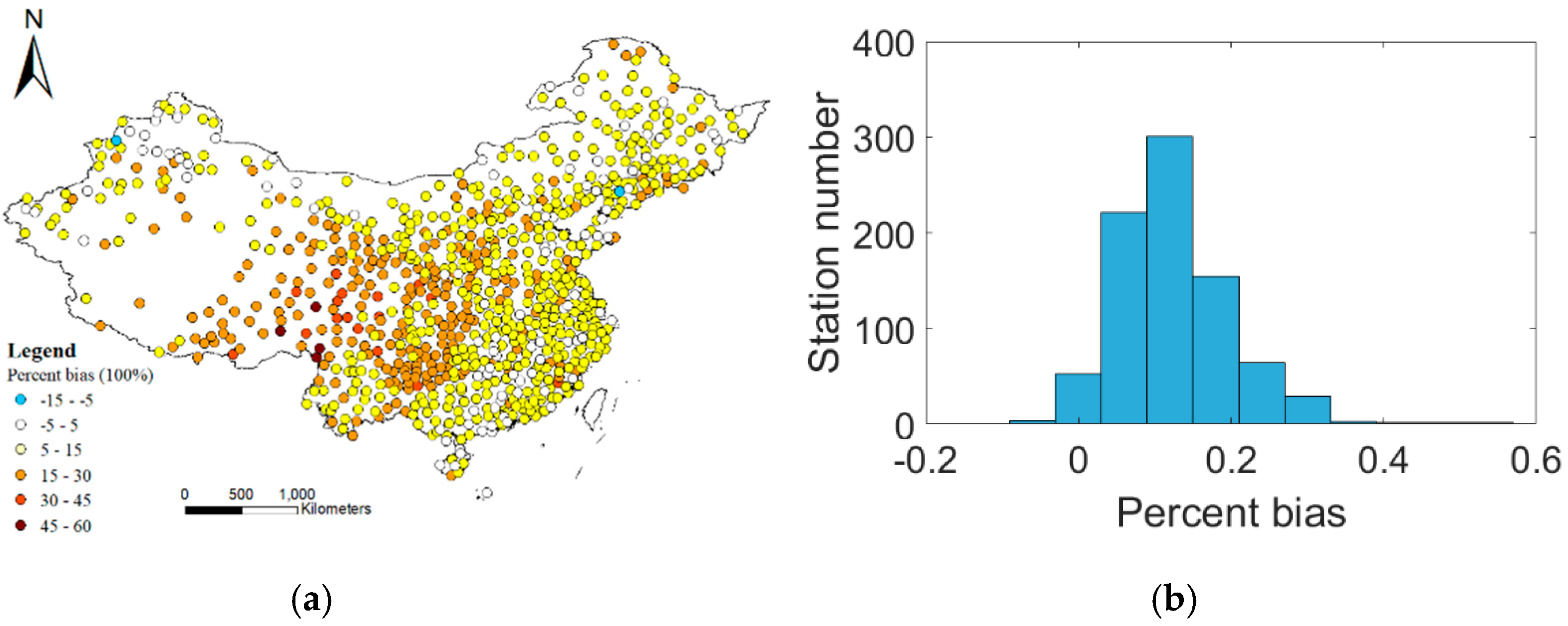
Figure 4 shows that the percentage bias for most stations is positive. This result indicates that average annual PET_cma is consistently overestimated; only two stations show an underestimate. The overall average percentage bias for the whole of China is 12.58%. Percentage bias varies spatially. The range 5% to 15% is the most frequent and is seen mainly in the east and north of China. In the west of inland China, percentage bias is mainly in the range 15% to 30%. There are a few stations in the west at high elevation with high PET_obs where percentage bias >30%.

Figure 5 shows the spatial distribution of the percentage bias of mean seasonal PET_cma. There are different seasonal features. Percentage bias is least in winter at 4.3% and greatest in spring at 15.7% compared to the percentage bias of mean annual PET_obs; the spring distribution shows more stations in southeast China with higher percentage bias (i.e., PET_cma is greatly overestimated), mainly in the range 15% to 30%. In summer, there are more stations in the west of China with higher percentage bias but fewer in southeast China, which is reflected in the frequency distribution showing that there are more stations in the percentage bias ranges 0–5% and >30%. In autumn, there are more stations in the northeast of China with percentage bias in the range −2% to 5%; the few stations with negative percentage bias represent that PET_cma is underestimated in comparison to PET_obs. In winter, PET_cma is overestimated in the south and underestimated in the north. The number of stations with percentage bias in the range −5% to 5% is greater than the annual average.

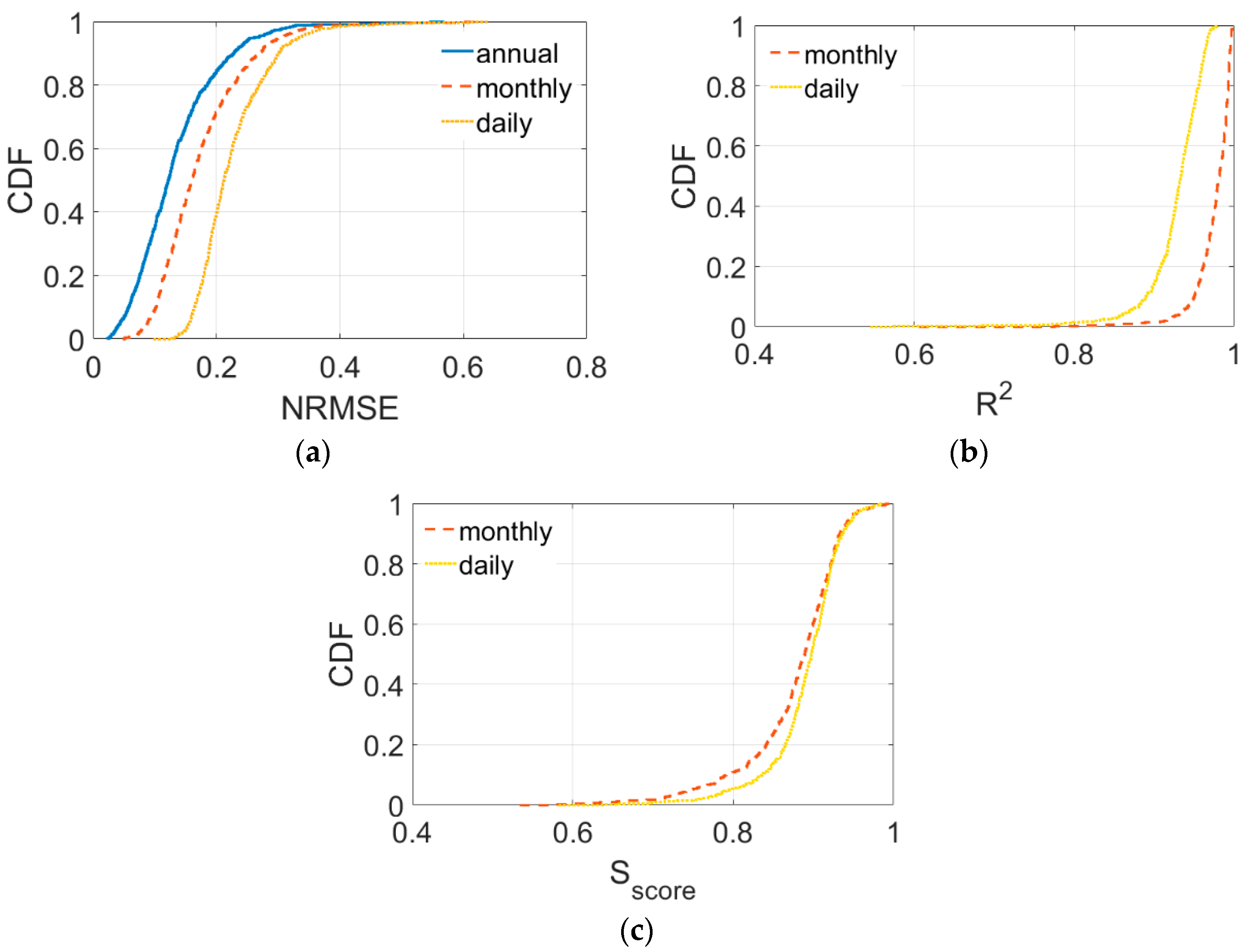
Percentage bias measures the trend of the average error distribution for a time series, but it cannot be used if there is a difference in time scales. The statistical measures NRMSE, R², and S_score are used to identify the variation in PET estimates with daily and monthly time scales. R² and S_score can be used to indicate differences at an annual scale, but the CMADS datasets cover only nine years, which is not long enough for adequate linear regression. Thus, annual behavior is only measured by NRMSE as reference. The three measures are used for all the stations. Figure 6 shows the cumulative distribution functions (CDF) of the measures for different time scales. The CDF for NMRSE shows that the estimate given by PET_cma is best at an annual time scale. It decreases as the time scale gets finer, but the difference is not very large. Almost 100% of the stations are <0.4 for every time scale. Up to 80% stations are <0.18, <0.23, and <0.27 for annual, monthly, and daily time scales, respectively. The R² values also show similar results for monthly and daily time scales with the monthly CDF better than the daily CDF. For 99% of the stations, monthly and daily R² values are >0.90 and >0.80. S_score shows that the difference between monthly and daily time scales is very small, but it has a broader range than the other two measures. The monthly and daily S_score values for most stations (99%) are >0.70 and >0.75, respectively.

3.3. Effect of Different Variables on the Bias in Estimation of the PET

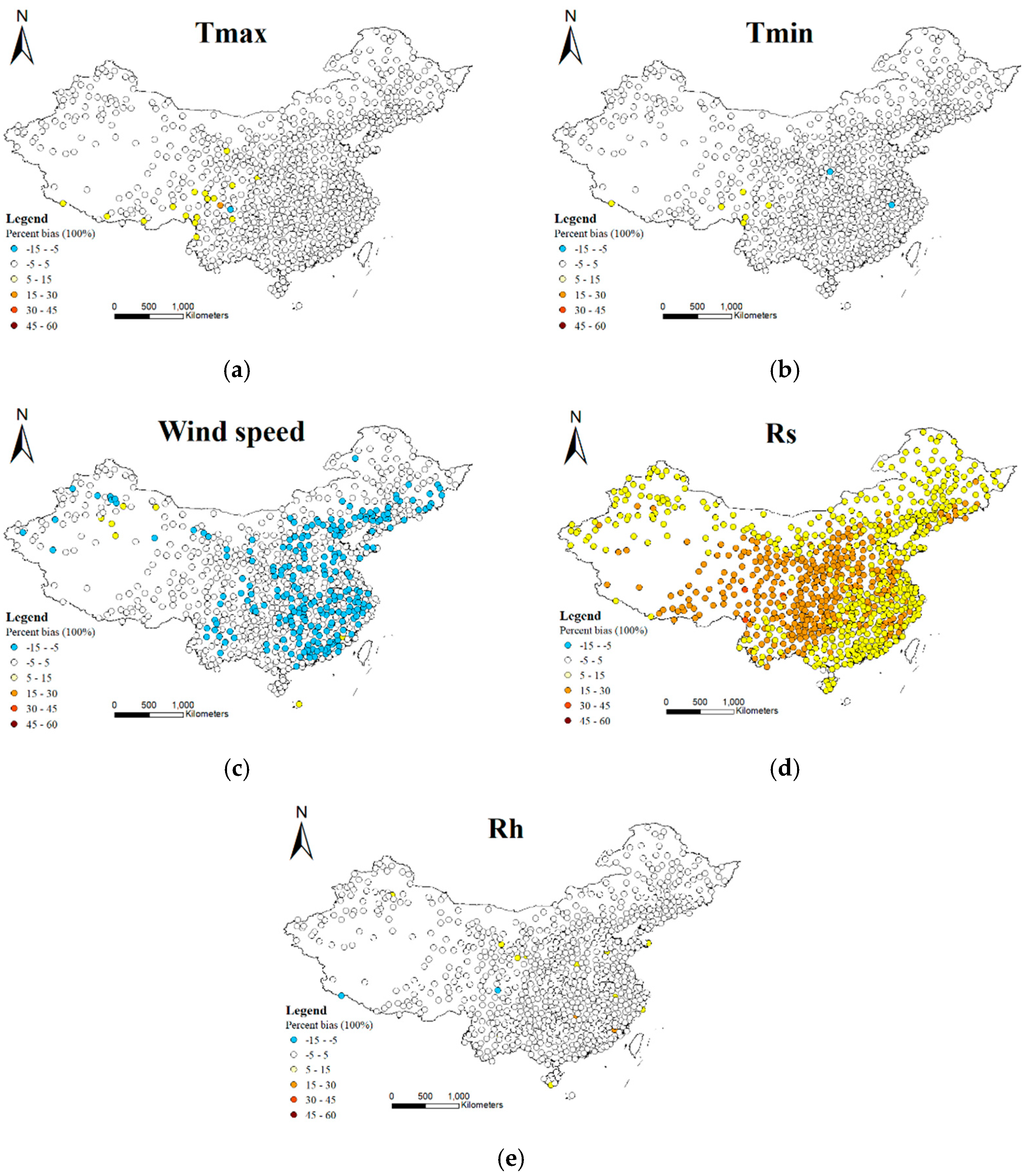
Figure 7 shows the contribution of each variable to the error in estimating mean annual PET_cma. Each is used in turn as an independent variable. PET_obs is the control variable. Percentage bias is the error measure. To estimate PET as a dependent variable, the observed data for one input variable of PM is replaced with reanalysis data from CMADS; all other input variables remain unchanged (i.e., they take the observed data used in the calculation of PET_obs). Percentage bias for most areas is in the range −5% to 5% when T_max, T_min, and R_h were the independent variables. This indicates that errors in T_max, T_min, and R_h from the CMADS data contributed little to the bias in PET_cma. Figure 7 shows that wind speed and solar radiation contribute to the error in PET_cma in different ways. When wind speed is the independent variable, PET is underestimated, and percentage bias is in the range −15% to −5%. Most underestimated values are found in eastern China. For solar radiation, R_s, PET is mainly overestimated with percentage bias in the range 5% to 30% over most of the area. In central and western China the overestimation is greater, with percentage bias predominantly in the range 15% to 30%.

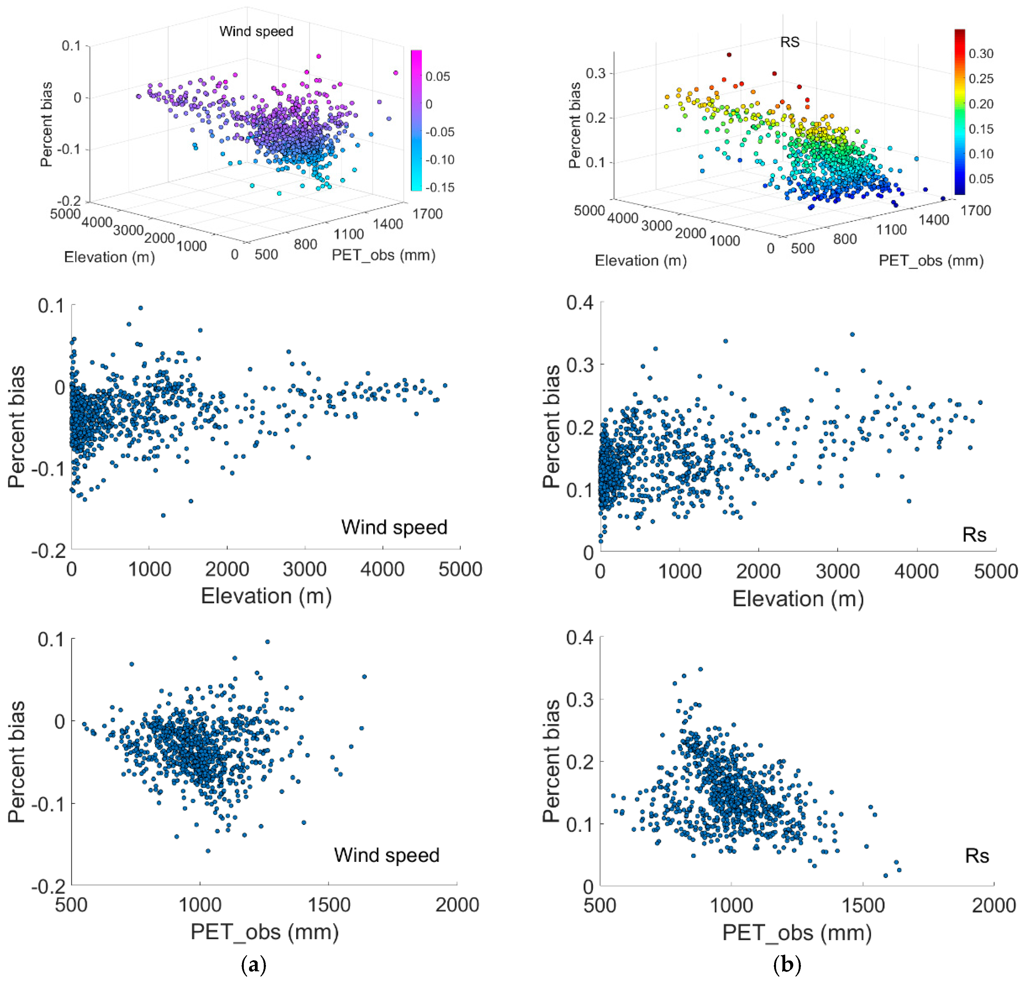
Elevation is commonly an important influence on wind speed and solar radiation. For example, topography influences wind speed when wind speed increase as air moves around a hill or along a narrow valley. The pressure gradient, friction due to the earth’s surface, and air density also influence wind speed. Figure 8 shows that when wind speed is the independent variable, the percentage bias is mainly <0. Bias <−10% is seen mainly at stations with elevation <2000 m when PET_obs is in the range 800–1300 mm. Solar radiation can be affected by atmospheric conditions, such as clouds and pollution, and topography can also cause substantial spatial variation in solar radiation [55]. PET was overestimated for most of the stations when R_s was the independent variable. When elevation increased, the lower boundary of percentage bias also increased. When elevation was >2000 m, the percentage bias of PET is >10%. Larger percentage bias, >20%, is found mainly for stations with PET_obs in the range 750–1250 mm. Windspeed, which causes underestimation of PET, and solar radiation, which causes overestimation of PET, offset each other, reducing the overestimation of PET_cma.

4. Discussion

This study evaluated the use of CMADS datasets in estimating PET across China during the period 2008–2016. As mentioned previously, there are alternative methods and different datasets for estimating PET. Weiland et al. [35] compared six different methods using Climate Forecast System Reanalysis (CFSR) data and evaluated the results against global Climate Research Unit (CRU) data. They noted that PM has high data demands and is sensitive to inaccuracies in the input data, and so recommended a re-calibrated form of the Hargreaves equation which gave global reference PET values that were comparable to CRU-derived values for many climate conditions. Lang [22] compared eight PET models with PM for southwestern China and found that the Makkink and Hargreaves–Samani methods are good alternatives to PM. Droogers and Allen [50] compared global PET predicted by PM and Hargreaves and recommended that the Hargreaves method be used in regions where accurate weather data cannot be expected because the method requires fewer climate variables as input, which makes it less sensitive to errors in climate data. Thus, the Hargreaves method has advantages in an area for which data is scarce, such as Africa [37].

PET is affected by many climatic factors. Liu et al. [56] analyzed the sensitivity of PET to meteorological data in China for the period 1960–2007. They found that the particular factor which is most sensitive differs across the country but nation-wide the most sensitive factor was, on average, vapor pressure. They also found some correlation between factor sensitivity and elevation. Yao et al. [57] used meteorological reanalysis datasets from the Environmental and Ecological Science Data Center for West China and found that solar radiation was the largest contributor to change in PET, and that wind speed most affected inter-annual variation of PET in China. Xu et al. [58] found that as well as solar radiation, atmospheric dynamics also strongly influence PET. Vegetation degradation in many regions of China is highly correlated with thermodynamic and physical land surface changes, which intensify the uneven spatial distribution of PET in China [59]. Gao et al. [60] analyzed PET from 580 stations in China for 1956–2000 and obtained similar results to ours: less solar radiation and decreased wind speed are major causes of reduced PET in most areas; and solar radiation, wind speed, and relative humidity have a greater effect than temperature on PET.

The overestimation of PET using the CMADS datasets is mainly due to the effect of solar radiation. Different methods in obtaining solar radiation need to be addressed. Solar radiation was calculated by Ångström–Prescott radiation equation for the station data, and Solar radiation of CMADS were obtained from radiance data of the International Satellite Cloud Climatology Project (ISCCP) with combination of data retrieved from the FY-2E satellite using the discrete-ordinate radiative transfer (DISTORT) model. For the satellite derived solar radiation, visible-band observations obtained from the FY2C geostationary meteorological satellite are used to generate hourly ground-incident solar radiation data with spatial resolution of 0.1° × 0.1°. The discrete ordinate method [61] was used to calculate radiation transfer in the inversion algorithm for the ground-incident solar radiation output. A 5-layer planoparallel ideal atmospheric model nonuniform in the vertical direction was designed, which consists of five solar spectral intervals (0.2–0.4, 0.4–0.5, 0.5–0.6, 0.6–0.7, 0.7–4.0 μm) to calculate the scattering, absorption, and reflection of solar radiation [39]. Although satellite-derived radiation has better spatial resolution, a study in Nigeria found that estimated solar radiation from the radiation equation model has a better error range and fits the ground measured data better than the satellite-derived data [62]. The ground measured, model estimated and satellite-derived solar radiation data can complement each other.

PET is important in water resources management and hydrological modeling. Overestimation of PET can lead to overestimating the severity of drought. Simulated discharge in hydrological models can also be affected by overestimated PET. Parmele [63] used a Hiemstra watershed model and two versions of the Stanford model and found that a constant bias of 20% in PET input data has a cumulative effect and results in considerable error in the computed hydrograph peaks and recessions. Other studies have found that parameter calibration can reduce errors from input data to some degree [64]. Oudin et al. [65] found that systematic errors in PET predictions have a greater impact than random errors, but that such errors are reduced by soil moisture accounting (SMA) using the GR4J model and TOPMODEL.

5. Conclusions

The CMADS reanalysis dataset is a useful alternative to observed weather data, especially in remote areas where observations are not easy to make. Evaluating PET calculated from the reanalysis dataset by comparing it with China-wide observations is important for the applicability of the CMADS dataset. This study used observed data from 836 weather stations across China to evaluate PET estimated by PM using CMADS data (PET_cma) by spatiotemporal comparison with PET_obs.

For the average annual PET, PET_cma and PET_obs agree well in their spatial distribution for most of China. PET_cma is an overestimation, compared to PET_obs, in western inland China with percentage bias in the range 15% to 30%. Average annual PET_obs is 1000 mm while average annual PET_cma is 1120 mm. Mean seasonal PET is overestimated, in comparison to PET_obs, for all four seasons, although the spatial distribution of PET_cma captures the general seasonal features. Average percentage bias is least in winter at 4.3% and greatest in spring at 15.7%. Mean seasonal PET estimates differ from mean annual PET estimates. In spring there are more stations in southeastern China for which PET_cma greatly overestimates. The percentage bias for a number of stations is mainly in the range 15% to 25%. In winter, there is overestimation in the south and underestimation in the north. The statistical measures NRMSE, R², and S_score consistently show that the annual PET_cma values are better than those at shorter time scales when compared with PET_obs.

Wind speed and solar radiation are the major variables that contribute to the errors in PET_cma but they each influence estimated PET in a different way. Wind speed causes an underestimation of PET with a percentage bias in the range −15% to −5%, with the largest errors being found in eastern China. Solar radiation causes an overestimation in the range 15% to 30% in central and western China. A larger percentage bias due to wind speed is found mainly at elevations below 2000 m while the larger percentage bias due to solar radiation is spread evenly across elevations. Underestimation of PET due to wind speed and overestimation of PET due to solar radiation are offset, reducing the overestimation of PET.

References

- Xu, C. Modelling the effects of climate change on water resources in central Sweden. Water Resour. Manag. 2000, 14, 177–189. [Google Scholar] [CrossRef]
- Tsakiris, G.; Vangelis, H. Establishing a drought index incorporating evapotranspiration. Eur. Water 2005, 9, 3–11. [Google Scholar]
- Miao, Q.; Rosa, R.D.; Shi, H.; Paredes, P.; Zhu, L.; Dai, J.; Gonçalves, J.M.; Pereira, L.S. Modeling water use, transpiration and soil evaporation of spring wheat–maize and spring wheat–sunflower relay intercropping using the dual crop coefficient approach. Agric. Water Manag. 2016, 165, 211–229. [Google Scholar] [CrossRef]
- Sprenger, M.; Leistert, H.; Gimbel, K.; Weiler, M. Illuminating hydrological processes at the soil–vegetation–atmosphere interface with water stable isotopes. Rev. Geophys. 2016, 54, 674–704. [Google Scholar] [CrossRef]
- Li, Z.; Zhang, Y.; Wang, S.; Yuan, G.; Yang, Y.; Cao, M. Evapotranspiration of a tropical rain forest in Xishuangbanna, southwest China. Hydrol. Process. 2010, 24, 2405–2416. [Google Scholar] [CrossRef]
- Zhang, B.; Kang, S.; Li, F.; Zhang, L. Comparison of three evapotranspiration models to Bowen ratio-energy balance method for a vineyard in an arid desert region of northwest China. Agric. For. Meteorol. 2008, 148, 1629–1640. [Google Scholar] [CrossRef]
- Xu, C.; Chen, D. Comparison of seven models for estimation of evapotranspiration and groundwater recharge using lysimeter measurement data in Germany. Hydrol. Process. 2005, 19, 3717–3734. [Google Scholar] [CrossRef]
- Samain, B.; Pauwels, V.R.N. Impact of potential and (scintillometer-based) actual evapotranspiration estimates on the performance of a lumped rainfall–runoff model. Hydrol. Earth Syst. Sci. 2013, 17, 4525–4540. [Google Scholar] [CrossRef] [Green Version]
- Audrézet, M.P.; Robaszkiewicz, M.; Mercier, B.; Nousbaum, J.B.; Bail, J.P.; Hardy, E.; Volant, A.; Lozac’H, P.; Charles, J.F.; Gouéron, H. Uncertainty analysis of computational methods for deriving sensible heat flux values from scintillometer measurements. Atmos. Meas. Tech. 2009, 2, 741–753. [Google Scholar] [Green Version]
- Wang, K.; Dickinson, R.E. A review of global terrestrial evapotranspiration: Observation, modeling, climatology, and climatic variability. Rev. Geophys. 2012, 50. [Google Scholar] [CrossRef] [Green Version]
- Zhang, K.; Kimball, J.S.; Running, S.W. A review of remote sensing based actual evapotranspiration estimation: A review of remote sensing evapotranspiration. WIREs Water 2016, 3, 834–853. [Google Scholar] [CrossRef]
- Long, D.; Longuevergne, L.; Scanlon, B.R. Uncertainty in evapotranspiration from land surface modeling, remote sensing, and GRACE satellites. Water Resour. Res. 2014, 50, 1131–1151. [Google Scholar] [CrossRef] [Green Version]
- Meng, X.; Ji, X.; Liu, Z.; Xiao, J.; Chen, X.; Wang, F. Research on improvement and application of snowmelt module in SWAT. J. Nat. Resour. 2014, 29, 528–539. [Google Scholar]
- Zhao, L.; Xia, J.; Xu, C.; Wang, Z.; Leszek, S.; Long, C. Evapotranspiration estimation methods in hydrological models. J. Geogr. Sci. 2013, 23, 359–369. [Google Scholar] [CrossRef]
- Lu, J.; Sun, G.; McNulty, S.G.; Amatya, D.M. A comparison of six potential evapotranspiration methods for regional use in the southeastern United States. J. Am. Water Resour. Assoc. 2005, 41, 621–633. [Google Scholar] [CrossRef]
- Muniandy, J.M.; Yusop, Z.; Askari, M. Evaluation of reference evapotranspiration models and determination of crop coefficient for Momordica charantia and Capsicum annuum. Agric. Water Manag. 2016, 169, 77–89. [Google Scholar] [CrossRef]
- Tabari, H.; Grismer, M.E.; Trajkovic, S. Comparative analysis of 31 reference evapotranspiration methods under humid conditions. Irrig. Sci. 2013, 31, 107–117. [Google Scholar] [CrossRef]
- Paparrizos, S.; Maris, F.; Matzarakis, A. Sensitivity analysis and comparison of various potential evapotranspiration formulae for selected Greek areas with different climate conditions. Theor. Appl. Climatol. 2017, 128, 745–759. [Google Scholar] [CrossRef]
- Arnold, J.G.; Srinivasan, R.; Muttiah, R.S.; Williams, J.R. Large area hydrologic modeling and assessment part I: Model development. J. Am. Water Resour. Assoc. 1998, 34, 73–89. [Google Scholar] [CrossRef]
- Liang, X.; Xie, Z.; Huang, M. A new parameterization for surface and groundwater interactions and its impact on water budgets with the variable infiltration capacity (VIC) land surface model. J. Geophys. Res. Atmos. 2003, 108. [Google Scholar] [CrossRef] [Green Version]
- Abbott, M.B.; Bathurst, J.C.; Cunge, J.A.; O’Connell, P.E.; Rasmussen, J. An introduction to the European hydrological system—Systeme Hydrologique Europeen, “SHE”, 1: History and philosophy of a physically-based, distributed modelling system. J. Hydrol. 1986, 87, 45–59. [Google Scholar] [CrossRef]
- Lang, D.; Zheng, J.; Shi, J.; Liao, F.; Ma, X.; Wang, W.; Chen, X.; Zhang, M. A comparative study of potential evapotranspiration estimation by eight methods with FAO Penman–Monteith method in southwestern China. Water 2017, 9, 734. [Google Scholar] [CrossRef]
- Kite, G.W.; Droogers, P. Comparing evapotranspiration estimates from satellites, hydrological models and field data. J. Hydrol. 2000, 229, 3–18. [Google Scholar] [CrossRef]
- Saha, S.; Moorthi, S.; Pan, H.-L.; Wu, X.; Wang, J.; Nadiga, S.; Tripp, P.; Kistler, R.; Woollen, J.; Behringer, D. The NCEP climate forecast system reanalysis. Bull. Am. Meteorol. Soc. 2010, 91, 1015–1058. [Google Scholar] [CrossRef]
- Kanamitsu, M.; Ebisuzaki, W.; Woollen, J.; Yang, S.-K.; Hnilo, J.J.; Fiorino, M.; Potter, G.L. NCEP–DOE AMIP-II Reanalysis (R-2). Bull. Am. Meteorol. Soc. 2002, 83, 1631–1644. [Google Scholar] [CrossRef]
- Kalnay, E.; Kanamitsu, M.; Kistler, R.; Collins, W.; Deaven, D.; Gandin, L.; Iredell, M.; Saha, S.; White, G.; Woollen, J.; et al. The NCEP/NCAR 40-year reanalysis project. Bull. Am. Meteorol. Soc. 1996, 77, 437–472. [Google Scholar] [CrossRef]
- Bromwich, D.H.; Wang, S.-H. Evaluation of the NCEP–NCAR and ECMWF 15- and 40-yr reanalysis using rawinsonde data from two independent Arctic field experiments. Mon. Weather Rev. 2005, 133, 3562–3578. [Google Scholar] [CrossRef]
- Uppala, S.M.; Kållberg, P.W.; Simmons, A.J.; Andrae, U.; Bechtold, V.D.C.; Fiorino, M.; Gibson, J.K.; Haseler, J.; Hernandez, A.; Kelly, G.A. The ERA-40 re-analysis. Q. J. R. Meteorol. Soc. 2005, 131, 2961–3012. [Google Scholar] [CrossRef] [Green Version]
- Dee, D.P.; Uppala, S.M.; Simmons, A.J.; Berrisford, P.; Poli, P.; Kobayashi, S.; Andrae, U.; Balmaseda, M.A.; Balsamo, G.; Bauer, P. The ERA-Interim reanalysis: Configuration and performance of the data assimilation system. Q. J. R. Meteorol. Soc. 2011, 137, 553–597. [Google Scholar] [CrossRef]
- Ebita, A.; Kobayashi, S.; Ota, Y.; Moriya, M.; Kumabe, R.; Onogi, K.; Harada, Y.; Yasui, S.; Miyaoka, K.; Takahashi, K.; et al. The Japanese 55-year reanalysis: An interim report. Sola 2011, 7, 149–152. [Google Scholar] [CrossRef]
- Rienecker, M.M.; Suarez, M.J.; Gelaro, R.; Todling, R.; Bacmeister, J.; Liu, E.; Bosilovich, M.G.; Schubert, S.D.; Takacs, L.; Kim, G.-K.; et al. MERRA: NASA’s Modern-Era Retrospective Analysis for Research and Applications. J. Clim. 2011, 24, 3624–3648. [Google Scholar] [CrossRef]
- Bao, X.; Zhang, F. Evaluation of NCEP–CFSR, NCEP–NCAR, ERA-Interim, and ERA-40 reanalysis datasets against independent sounding observations over the Tibetan plateau. J. Clim. 2013, 26, 206–214. [Google Scholar] [CrossRef]
- Lindsay, R.; Wensnahan, M.; Schweiger, A.; Zhang, J. Evaluation of seven different atmospheric reanalysis products in the Arctic. J. Clim. 2014, 27, 2588–2606. [Google Scholar] [CrossRef]
- Ma, L.; Zhang, T.; Li, Q.; Frauenfeld, O.W.; Qin, D. Evaluation of ERA-40, NCEP-1, and NCEP-2 reanalysis air temperatures with ground-based measurements in China. J. Geophys. Res. Atmos. 2008, 113. [Google Scholar] [CrossRef] [Green Version]
- Weiland, F.C.S.; Tisseuil, C.; Dürr, H.H.; Vrac, M.; Beek, L.P.H.V. Selecting the optimal method to calculate daily global reference potential evaporation from CFSR reanalysis data for application in a hydrological model study. Hydrol. Earth Syst. Sci. 2012, 16, 983–1000. [Google Scholar] [CrossRef] [Green Version]
- Srivastava, P.K.; Han, D.; Ramirez, M.A.R.; Islam, T. Comparative assessment of evapotranspiration derived from NCEP and ECMWF global datasets through weather research and forecasting model. Atmos. Sci. Lett. 2013, 14, 118–125. [Google Scholar] [CrossRef]
- Trambauer, P.; Dutra, E.; Maskey, S.; Werner, M.; Pappenberger, F.; Van Beek, L.P.H.; Uhlenbrook, S. Comparison of different evaporation estimates over the African continent. Hydrol. Earth Syst. Sci. 2014, 18, 193–212. [Google Scholar] [CrossRef] [Green Version]
- Meng, X.; Wang, H.; Wu, Y.; Long, A.; Wang, J.; Shi, C.; Ji, X. Investigating spatiotemporal changes of the land-surface processes in Xinjiang using high-resolution CLM3.5 and CLDAS: Soil temperature. Sci. Rep. 2017, 7, 13286. [Google Scholar] [CrossRef] [PubMed] [Green Version]
- Shi, C.; Xie, Z.; Hui, Q.; Liang, M.; Yang, X. China land soil moisture ENKF data assimilation based on satellite remote sensing data. Sci. China Earth Sci. 2011, 54, 1430–1440. [Google Scholar] [CrossRef]
- Zhang, T. Multi-Source Data Fusion and Application Research Base on LAPS/STMAS. Master’s Thesis, Nanjing University of Information Science & Technology, Nanjing, China, 2013. (In Chinese). [Google Scholar]
- Meng, X.; Wang, H. Significance of the China Meteorological Assimilation Driving Datasets for the SWAT Model (CMADS) of East Asia. Water 2017, 9, 765. [Google Scholar] [CrossRef]
- Meng, X.; Wang, H.; Lei, X.; Cai, S.; Wu, H.; Ji, X.; Wang, J. Hydrological modeling in the Manas river basin using soil and water assessment tool driven by CMADS. Teh. Vjesn. 2017, 24, 525–534. [Google Scholar]
- Meng, X.; Yu, D.; Liu, Z. Energy balance-based swat model to simulate the mountain snowmelt and runoff—Taking the application in Juntanghu watershed (China) as an example. J. Mt. Sci. 2015, 12, 368–381. [Google Scholar] [CrossRef]
- Meng, X.; Wang, H.; Cai, S.; Zhang, X.; Leng, G.; Lei, X.; Shi, C.; Liu, S.; Shang, Y. The China meteorological assimilation driving datasets for the SWAT model (CMADS) application in China: A case study in Heihe river basin. Preprints 2016, 37, 1–19. [Google Scholar]
- Zhao, F.; Wu, Y. Parameter uncertainty analysis of the SWAT Model in a Mountain Loess transitional watershed on the Chinese Loess Plateau. Water 2018, 10, 690. [Google Scholar] [CrossRef]
- Vu, T.T.; Li, L.; Jun, K.S. Evaluation of multi satellite precipitation products for streamflow simulations: A case study for the Han river basin in the Korean peninsula, east Asia. Water 2018, 10, 642. [Google Scholar] [CrossRef]
- Liu, J.; Shanguan, D.; Liu, S.; Ding, Y. Evaluation and hydrological simulation of CMADS and CFSR reanalysis datasets in the Qinghai Tibet Plateau. Water 2018, 10, 513. [Google Scholar] [CrossRef]
- Cao, Y.; Zhang, J.; Yang, M. Application of SWAT model with CMADS data to estimate hydrological elements and parameter uncertainty based on SUFI-2 Algorithm in the Lijiang river basin, China. Water 2018, 10, 742. [Google Scholar] [CrossRef]
- Shao, G.; Guan, Y.; Zhang, D.; Yu, B.; Zhu, J. The impacts of climate variability and land use change on streamflow in the Hailiutu river basin. Water 2018, 10, 814. [Google Scholar] [CrossRef]
- Allen, R.G.; Pereira, L.S.; Raes, D.; Smith, M. Crop Evapotranspiration—Guidelines for Computing Crop Water Requirements; FAO Irrigation and Drainage Paper 56; Food and Agriculture Organization of the United Nations (FAO): Rome, Italy, 1998. [Google Scholar]
- Monteith, J.L. Evaporation and environment. Symp. Soc. Exp. Biol. 1965, 19, 205–234. [Google Scholar] [PubMed]
- Gong, L.; Xu, C.; Chen, D.; Halldin, S.; Chen, Y. Sensitivity of the Penman–Monteith reference evapotranspiration to key climatic variables in the Changjiang (Yangtze River) basin. J. Hydrol. 2006, 329, 620–629. [Google Scholar] [CrossRef]
- Yang, Y.; Cui, Y.; Luo, Y.; Lyu, X.; Traore, S.; Khan, S.; Wang, W. Short-term forecasting of daily reference evapotranspiration using the Penman-Monteith model and public weather forecasts. Agric. Water Manag. 2016, 177, 329–339. [Google Scholar] [CrossRef]
- Almorox, J.; Senatore, A.; Quej, V.H.; Mendicino, G. Worldwide assessment of the Penman–Monteith temperature approach for the estimation of monthly reference evapotranspiration. Theor. Appl. Climatol. 2016, 131, 1–11. [Google Scholar] [CrossRef]
- Kang, S.; Kim, S.; Lee, D. Spatial and temporal patterns of solar radiation based on topography a. Can. J. For. Res. 2002, 32, 487–497. [Google Scholar] [CrossRef]
- Droogers, P.; Allen, R.G. Estimating reference evapotranspiration under inaccurate data conditions. Irrig. Drain. Syst. 2002, 16, 33–45. [Google Scholar] [CrossRef]
- Liu, C.; Zhang, D.; Liu, X.; Zhao, C. Spatial and temporal change in the potential evapotranspiration sensitivity to meteorological factors in China (1960–2007). J. Geogr. Sci. 2012, 22, 3–14. [Google Scholar] [CrossRef] [Green Version]
- Yao, Y.; Zhao, S.; Zhang, Y.; Jia, K.; Liu, M. Spatial and decadal variations in potential evapotranspiration of China based on reanalysis datasets during 1982–2010. Atmosphere 2014, 5, 737–754. [Google Scholar] [CrossRef]
- Xu, X. Analyzing potential evapotranspiration and climate drivers in China. Chin. J. Geophys. 2011, 54, 125–134. [Google Scholar] [CrossRef]
- Gao, G.; Chen, D.; Ren, G.; Chen, Y.; Liao, Y. Spatial and temporal variations and controlling factors of potential evapotranspiration in China: 1956–2000. J. Geogr. Sci. 2006, 16, 3–12. [Google Scholar] [CrossRef]
- Stamnes, K.; Tsay, S.C.; Wiscombe, W.; Jayaweera, K. Numerically stable algorithm for discrete ordinate method radiative transfer in multiple scattering and emitting layered media. Appl. Opt. 1988, 27, 502–509. [Google Scholar] [CrossRef] [PubMed]
- Olomiyesan, B.M.; Oyedum, O.D. Comparative study of ground measured, satellite-derived, and estimated global solar radiation data in Nigeria. J. Sol. Energy 2016, 3, 1–7. [Google Scholar] [CrossRef]
- Parmele, L.H. Errors in output of hydrologic models due to errors in input potential evapotranspiration. Water Resour. Res. 1972, 8, 348–359. [Google Scholar] [CrossRef]
- Andréassian, V.; Perrin, C.; Michel, C. Impact of imperfect potential evapotranspiration knowledge on the efficiency and parameters of watershed models. J. Hydrol. 2004, 286, 19–35. [Google Scholar] [CrossRef]
- Oudin, L.; Perrin, C.; Mathevet, T.; Andréassian, V.; Michel, C. Impact of biased and randomly corrupted inputs on the efficiency and the parameters of watershed models. J. Hydrol. 2006, 320, 62–83. [Google Scholar] [CrossRef]
Figure 1.
Spatial distribution of weather stations in China.
Figure 2.
Average annual PET_obs (a) and PET_cma (b) across China, with their histograms (c).
Figure 3.
Mean seasonal potential evapotranspiration estimated from weather station data (PET_obs, (a)), CMADS datasets (PET_cma, (b)) with their histograms (c).
Figure 4.
Spatial distribution of percentage bias, indicating the accuracy of average annual PET_cma values (a), and frequency distribution of percentage bias (b).
Figure 5.
Spatial distribution of percentage bias showing the accuracy of mean seasonal potential evapotranspiration (PET) estimated using CMADS datasets, PET_cma (a) and the frequency distribution of percentage bias (b).
Figure 6.
Cumulative distribution functions of the statistical measures NRMSE (a), R2 (b), and Sscore (c) indicating the accuracy of monthly and daily PET_cma estimates compared to PET_obs.
Figure 7.
Spatial distribution of percentage bias showing the effects of maximum temperature (a), minimum temperature (b), wind speed (c), solar radiation (d), and relative humidity (e) on the bias of PET_cma.
Figure 8.
Relationship between elevation, PET_obs, and errors indicated by percentage bias for wind speed (a) and solar radiation (b).
© 2018 by the authors. Licensee MDPI, Basel, Switzerland. This article is an open access article distributed under the terms and conditions of the Creative Commons Attribution (CC BY) license (http://creativecommons.org/licenses/by/4.0/).
Share and Cite
MDPI and ACS Style
Tian, Y.; Zhang, K.; Xu, Y.-P.; Gao, X.; Wang, J. Evaluation of Potential Evapotranspiration Based on CMADS Reanalysis Dataset over China. Water 2018, 10, 1126. https://doi.org/10.3390/w10091126
AMA Style
Tian Y, Zhang K, Xu Y-P, Gao X, Wang J. Evaluation of Potential Evapotranspiration Based on CMADS Reanalysis Dataset over China. Water. 2018; 10(9):1126. https://doi.org/10.3390/w10091126
Chicago/Turabian StyleTian, Ye, Kejun Zhang, Yue-Ping Xu, Xichao Gao, and Jie Wang. 2018. "Evaluation of Potential Evapotranspiration Based on CMADS Reanalysis Dataset over China" Water 10, no. 9: 1126. https://doi.org/10.3390/w10091126
Note that from the first issue of 2016, this journal uses article numbers instead of page numbers. See further details here.