Modelling Spatiotemporal Dynamics of Large Wood Recruitment, Transport, and Deposition at the River Reach Scale during Extreme Floods

 ,
,
Abstract
:
1. Introduction
2. Methods
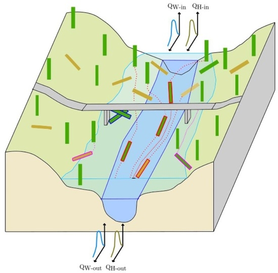
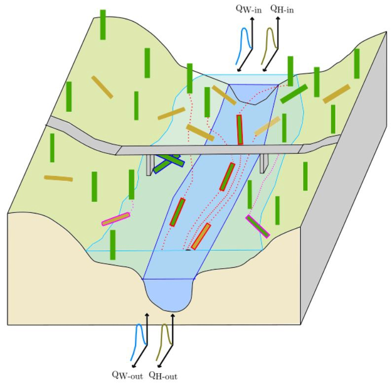
2.1. Basic Framework of LWD Modelling
2.2. Identification and Classification of Trees
2.3. Hydrodynamic Simulation
2.4. LWD Simulation
- Localization: For every tree, its closest 3 mesh-nodes of the hydrodynamic model are identified. On these nodes, the hydrodynamic conditions of the particular time step are read out. The conditions are interpolated at the position of the tree using the inverse distance weighting interpolation method.
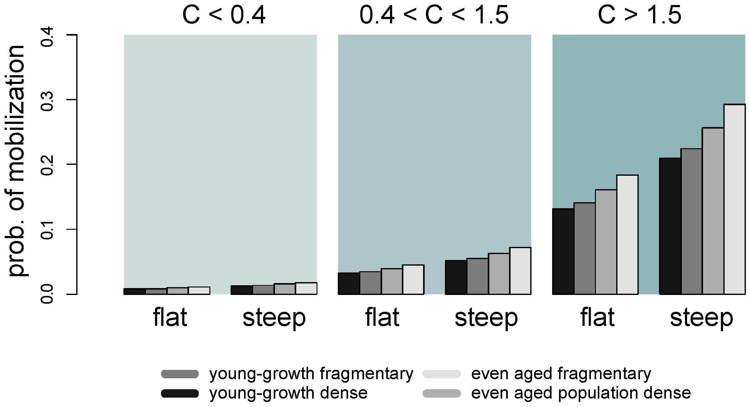
- Recruitment and mobilization: Whether standing trees are standing or have fallen into the channel is checked. For standing trees, the hydrodynamic forces are analyzed to estimate the recruitment. For uprooted trees, the recruitment analysis is not needed and the flow conditions are analyzed; only recruitment processes from soil erosion in the influence zone of the flood are considered. Lateral erosion of river banks and subsequent river widening or other changes of the channel morphology are not considered. Since there is still a lack of detailed knowledge with respect to possible recruitment mechanisms, a probabilistic approach is considered. Depending on the hydrodynamic forces acting on a tree, a recruitment probability is determined on the basis of the vegetation structure and the local slope according to [59]. In a first step, the hydraulic impact C is calculated on the basis of flow depth h and flow velocity U (Equation (2)).
- On the basis of the classified hydraulic impact, the wood structure, and the slope, a probability factor of recruitment is assigned (Figure 2). The probability of mobilization is calculated for each time step, divided by the total number of time steps. For each tree, it is randomly defined if the status of the tree changes from “standing” to “recruited,” depending on the assigned probability. A “recruited” tree is defined as an uprooted tree that has fallen due to hydrodynamic forces.
- Entrainment, transport, and deposition: For all lying trees (uprooted greenwood and deadwood), it is checked whether the conditions for entrainment are fulfilled. For simplicity, it is assumed that the density of all trees is lower than 1 and their orientation is parallel to the flow. Interactions between trees and breaking of logs are neglected. The transport process can take place under floating or rolling/sliding conditions [89]. Depending on these conditions, the transport velocity differs from a velocity equal to the streamflow for floating trees to reduced velocity for sliding or rolling trees. For a comprehensive description of the physical foundations of the transport dynamics, we refer to the literature [59]. Using the information about velocity and flow direction, the new positions for every transported log are calculated for every time step. A transported log can be deposited at a particular time step if the conditions for transportation are not fulfilled anymore, and it can be remobilized at a later time step. Transported trees that are not deposited or entrapped at a bridge reach the lower system boundary (LSB) and are not considered in the further simulation.
- Bridge clogging: Bridges can optionally be considered in the model as polygon geometries with information about their height above the riverbed and length. If 1 or more of the 3 closest mesh-nodes of a transported tree lies within such a polygon, it is assumed that the tree is passing a bridge. In this case, it can collide with 1 or more piers or interact with the bridge deck and cause clogging [90]. As a simplification, the specific bridge structure and the flow conditions are neglected. Furthermore, if log jams are formed, they do not interact with other trees and cannot break. With regard to the randomness of this process and the lack of physical knowledge, a probabilistic approach is applied. According to [90], the probability of a log being jammed at a bridge is the sum of all blocking probabilities on single bridge elements. The blocking probability for the piers is calculated following [91] since only the bottom width and log length are considered in the equation. The clogging probability at the bridge piers is calculated according to [92] (Equation (3)) and at the bridge deck according to [93] for trees with (Equation (4)) and without (Equation (5)) rootstocks. The total blocking probability of a tree at a bridge is the sum of the single probabilities. A random generator is used to determine, with the given probability, whether a tree is jammed or passes the bridge normally. For a detailed description of the clogging probabilities, we refer to [91]. This feature considering LW retention by clogging is optional.
2.5. Model Test
2.6. Modelling LWD during an Extreme Flood
3. Results
4. Discussion and Conclusions
Supplementary Materials
Author Contributions
Funding
Acknowledgments
Conflicts of Interest
References
- Desai, B.; Maskrey, A.; Peduzzi, P.; De Bono, A.; Herold, C. Making Development Sustainable: The Future of Disaster Risk Management, Global Assessment Report on Disaster Risk Reduction; United Nations Office for Disaster Risk Reduction (UNISDR): Geneva, Switzerland, 2015. [Google Scholar]
- Weingartner, R.; Barben, M.; Spreafico, M. Floods in mountain areas—An overview based on examples from Switzerland. Mt. Hydrol. Water Resour. 2003, 282, 10–24. [Google Scholar] [CrossRef]
- Zischg, A. Floodplains and Complex Adaptive Systems—Perspectives on Connecting the Dots in Flood Risk Assessment with Coupled Component Models. Systems 2018, 6, 9. [Google Scholar] [CrossRef]
- Zischg, A.P.; Hofer, P.; Mosimann, M.; Röthlisberger, V.; Ramirez, J.A.; Keiler, M.; Weingartner, R. Flood risk (d)evolution: Disentangling key drivers of flood risk change with a retro-model experiment. Sci. Total Environ. 2018, 639, 195–207. [Google Scholar] [CrossRef] [PubMed]
- Ruiz-Villanueva, V.; Wyżga, B.; Mikuś, P.; Hajdukiewicz, M.; Stoffel, M. Large wood clogging during floods in a gravel-bed river: The Długopole bridge in the Czarny Dunajec River, Poland. Earth Surf. Process. Landf. 2017, 42, 516–530. [Google Scholar] [CrossRef]
- Kim, H.J.; Lee, J.W.; Yoon, K.S.; Cho, Y.S. Numerical analysis of flood risk change due to obstruction. KSCE J. Civ. Eng. 2012, 16, 207–214. [Google Scholar] [CrossRef]
- Ruiz-Villanueva, V.; Bodoque, J.M.; Díez-Herrero, A.; Eguibar, M.A.; Pardo-Igúzquiza, E. Reconstruction of a flash flood with large wood transport and its influence on hazard patterns in an ungauged mountain basin. Hydrol. Process. 2013, 27, 3424–3437. [Google Scholar] [CrossRef]
- Ruiz-Villanueva, V.; Bodoque, J.M.; Díez-Herrero, A.; Bladé, E. Large wood transport as significant influence on flood risk in a mountain village. Nat. Hazards 2014, 74, 967–987. [Google Scholar] [CrossRef]
- Hajdukiewicz, H.; Wyżga, B.; Mikuś, P.; Zawiejska, J.; Radecki-Pawlik, A. Impact of a large flood on mountain river habitats, channel morphology, and valley infrastructure. Floods Mt. Environ. 2016, 272, 55–67. [Google Scholar] [CrossRef]
- Loat, R.; Petraschek, A. Consideration of Flood Hazards for Activities with Spatial Impact; Federal Office for the Environment (FOEN): Bern, Switzerland, 1997. [Google Scholar]
- Mazzorana, B.; Fuchs, S. Fuzzy Formative Scenario Analysis for woody material transport related risks in mountain torrents. Environ. Model. Softw. 2010, 25, 1208–1224. [Google Scholar] [CrossRef]
- Mazzorana, B.; Comiti, F.; Scherer, C.; Fuchs, S. Developing consistent scenarios to assess flood hazards in mountain streams. J. Environ. Manag. 2012, 94, 112–124. [Google Scholar] [CrossRef] [PubMed]
- Schmocker, L.; Weitbrecht, V. Driftwood: Risk Analysis and Engineering Measures. J. Hydraul. Eng. 2013, 139, 683–695. [Google Scholar] [CrossRef]
- Vetsch, D.; Siviglia, A.; Ehrbar, D.; Facchini, M.; Gerber, M.; Kammerer, S.; Peter, S.; Vonwiler, L.; Volz, C.; Farshi, D.; et al. BASEMENT—Basic Simulation Environment for Computation of Environmental Flow and Natural Hazard Simulation; Eidgenössische Technische Hochschule (ETH) Zurich: Zurich, Switzerland, 2017. [Google Scholar]
- Horton, P.; Jaboyedoff, M.; Rudaz, B.; Zimmermann, M. Flow-R, a model for susceptibility mapping of debris flows and other gravitational hazards at a regional scale. Nat. Hazards Earth Syst. Sci. 2013, 13, 869–885. [Google Scholar] [CrossRef] [Green Version]
- Coulthard, T.J.; Neal, J.C.; Bates, P.D.; Ramirez, J.; de Almeida, G.A.M.; Hancock, G.R. Integrating the LISFLOOD-FP 2D hydrodynamic model with the CAESAR model: Implications for modelling landscape evolution. Earth Surf. Process. Landf. 2013, 38, 1897–1906. [Google Scholar] [CrossRef]
- Gurnell, A.M.; Piegay, H.; Swanson, F.J.; Gregory, S.V. Large wood and fluvial processes. Freshw. Biol. 2002, 47, 601–619. [Google Scholar] [CrossRef]
- Wohl, E. Of wood and rivers: Bridging the perception gap. WIREs Water 2015, 2, 167–176. [Google Scholar] [CrossRef]
- Wohl, E. Bridging the gaps: An overview of wood across time and space in diverse rivers. Geomorphology 2017, 279, 3–26. [Google Scholar] [CrossRef]
- Moulin, B.; Schenk, E.R.; Hupp, C.R. Distribution and characterization of in-channel large wood in relation to geomorphic patterns on a low-gradient river. Earth Surf. Process. Landf. 2011, 36, 1137–1151. [Google Scholar] [CrossRef]
- Sear, D.A.; Millington, C.E.; Kitts, D.R.; Jeffries, R. Logjam controls on channel-floodplain interactions in wooded catchments and their role in the formation of multi-channel patterns. Geomorphology 2010, 116, 305–319. [Google Scholar] [CrossRef]
- Senter, A.E.; Pasternack, G.B.; Piégay, H.; Vaughan, M.C.; Lehyan, J.S. Wood export varies among decadal, annual, seasonal, and daily scale hydrologic regimes in a large, Mediterranean climate, mountain river watershed. Geomorphology 2017, 276, 164–179. [Google Scholar] [CrossRef] [Green Version]
- Seo, J.I.; Nakamura, F. Scale-dependent controls upon the fluvial export of large wood from river catchments. Earth Surf. Process. Landf. 2009, 34, 786–800. [Google Scholar] [CrossRef]
- Seo, J.I.; Nakamura, F.; Nakano, D.; Ichiyanagi, H.; Chun, K.W. Factors controlling the fluvial export of large woody debris, and its contribution to organic carbon budgets at watershed scales. Water Resour. Res. 2008, 44. [Google Scholar] [CrossRef] [Green Version]
- Kramer, N.; Wohl, E. Rules of the road: A qualitative and quantitative synthesis of large wood transport through drainage networks. Geomorphology 2017, 279, 74–97. [Google Scholar] [CrossRef]
- Ruiz-Villanueva, V.; PIEGAY, H.; Stoffel, M.; Gaertner, V.; Perret, F. Analysis of Wood Density to Improve Understanding of Wood Buoyancy in Rivers. In Engineering Geology for Society and Territory-Volume 3; Lollino, G., Arattano, M., Rinaldi, M., Giustolisi, O., Marechal, J.C., Grant, G.E., Eds.; Springer International Publishing: Cham, Switzerland, 2015; pp. 163–166. [Google Scholar]
- Ruiz-Villanueva, V.; Piégay, H.; Gurnell, A.A.; Marston, R.A.; Stoffel, M. Recent advances quantifying the large wood dynamics in river basins: New methods and remaining challenges. Rev. Geophys. 2016, 54, 611–652. [Google Scholar] [CrossRef] [Green Version]
- Ruiz-Villanueva, V.; Wyżga, B.; Hajdukiewicz, H.; Stoffel, M. Exploring large wood retention and deposition in contrasting river morphologies linking numerical modelling and field observations. Earth Surf. Process. Landf. 2016, 41, 446–459. [Google Scholar] [CrossRef]
- Gurnell, A.M.; Petts, G.E.; Hannah, D.M.; Smith, B.P.G.; Edwards, P.J.; Kollmann, J.; Ward, J.V.; Tockner, K. Wood storage within the active zone of a large European gravel-bed river. Geomorphology 2000, 34, 55–72. [Google Scholar] [CrossRef]
- Gurnell, A.M.; Petts, G.E.; Harris, N.; Ward, J.V.; Tockner, K.; Edwards, P.J.; Kollmann, J. Large wood retention in river channels: The case of the Fiume Tagliamento, Italy. Earth Surf. Process. Landf. 2000, 25, 255–275. [Google Scholar] [CrossRef]
- Wohl, E.; Cenderelli, D.A.; Dwire, K.A.; Ryan-Burkett, S.E.; Young, M.K.; Fausch, K.D. Large in-stream wood studies: A call for common metrics. Earth Surf. Process. Landf. 2010, 35, 618–625. [Google Scholar] [CrossRef]
- Seo, J.I.; Nakamura, F.; Chun, K.W.; Kim, S.W.; Grant, G.E. Precipitation patterns control the distribution and export of large wood at the catchment scale. Hydrol. Process. 2015, 29, 5044–5057. [Google Scholar] [CrossRef] [Green Version]
- MacVicar, B.J.; Piégay, H.; Henderson, A.; Comiti, F.; Oberlin, C.; Pecorari, E. Quantifying the temporal dynamics of wood n large rivers: Field trials of wood surveying, a-ting, tracking, and monitoring techniques. Earth Surf. Process. Landf. 2009, 34, 2031–2046. [Google Scholar] [CrossRef]
- Kramer, N.; Wohl, E. Estimating fluvial wood discharge using time-lapse photography with varying sampling intervals. Earth Surf. Process. Landf. 2014, 39, 844–852. [Google Scholar] [CrossRef]
- Ravazzolo, D.; Mao, L.; Picco, L.; Sitzia, T.; Lenzi, M.A. Geomorphic effects of wood quantity and characteristics in three Italian gravel-bed rivers. Geomorphology 2015, 246, 79–89. [Google Scholar] [CrossRef]
- Schenk, E.R.; Moulin, B.; Hupp, C.R.; Richter, J.M. Large wood budget and transport dynamics on a large river using radio telemetry. Earth Surf. Process. Landf. 2014, 39, 487–498. [Google Scholar] [CrossRef]
- Bertoldi, W.; Ashmore, P.; Tubino, M. A method for estimating the mean bed load flux in braided rivers. Geomorphology 2009, 103, 330–340. [Google Scholar] [CrossRef]
- Bertoldi, W.; Gurnell, A.A.; Welber, M. Wood recruitment and retention: The fate of eroded trees on a braided river explored using a combination of field and remotely-sensed data sources. Geomorphology 2013, 180, 146–155. [Google Scholar] [CrossRef]
- Brown, C.G.; Sarabandi, K.; Pierce, L.E. Model-Based Estimation of Forest Canopy Height in Red and Austrian Pine Stands Using Shuttle Radar Topography Mission and Ancillary Data: A Proof-of-Concept Study. IEEE Trans. Geosci. Remote Sens. 2010, 48, 1105–1118. [Google Scholar] [CrossRef] [Green Version]
- Henshaw, A.J.; Bertoldi, W.; Harvey, G.L.; Gurnell, A.M.; Welber, M. Large Wood Dynamics Along the Tagliamento River, Italy: Insights from Field and Remote Sensing Investigations. In Engineering Geology for Society and Territory-Volume 3; Lollino, G., Arattano, M., Rinaldi, M., Giustolisi, O., Marechal, J.C., Grant, G.E., Eds.; Springer International Publishing: Cham, Switzerland, 2015; pp. 151–154. [Google Scholar]
- Ravazzolo, D.; Mao, L.; Picco, L.; Lenzi, M.A. Tracking log displacement during floods in the Tagliamento River using RFID and GPS tracker devices. Geomorphology 2015, 228, 226–233. [Google Scholar] [CrossRef]
- MacVicar, B.; Piégay, H. Implementation and validation of video monitoring for wood budgeting in a wandering piedmont river, the Ain River (France). Earth Surf. Process. Landf. 2012, 37, 1272–1289. [Google Scholar] [CrossRef]
- Benacchio, V.; Piégay, H.; Buffin-Bélanger, T.; Vaudor, L. A new methodology for monitoring wood fluxes in rivers using a ground camera: Potential and limits. Geomorphology 2017, 279, 44–58. [Google Scholar] [CrossRef]
- Wyżga, B.; Mikuś, P.; Zawiejska, J.; Ruiz-Villanueva, V.; Kaczka, R.J.; Czech, W. Log transport and deposition in incised, channelized, and multithread reaches of a wide mountain river: Tracking experiment during a 20-year flood. Geomorphology 2017, 279, 98–111. [Google Scholar] [CrossRef]
- Comiti, F.; Lucía, A.; Rickenmann, D. Large wood recruitment and transport during large floods: A review. Geomorphology 2016, 269, 23–39. [Google Scholar] [CrossRef]
- Mazzorana, B.; Zischg, A.; Largiader, A.; Hübl, J. Hazard index maps for woody material recruitment and transport in alpine catchments. Nat. Hazards Earth Syst. Sci. 2009, 9, 197–209. [Google Scholar] [CrossRef] [Green Version]
- Wohl, E. Threshold-induced complex behavior of wood in mountain streams. Geology 2011, 39, 587–590. [Google Scholar] [CrossRef]
- Staffler, H.; Pollinger, R.; Zischg, A.; Mani, P. Spatial variability and potential impacts of climate change on flood and debris flow hazard zone mapping and implications for risk management. Nat. Hazards Earth Syst. Sci. 2008, 8, 539–558. [Google Scholar] [CrossRef] [Green Version]
- Ruiz-Villanueva, V.; Wyżga, B.; Mikuś, P.; Hajdukiewicz, H.; Stoffel, M. The role of flood hydrograph in the remobilization of large wood in a wide mountain river. J. Hydrol. 2016, 541, 330–343. [Google Scholar] [CrossRef]
- Ruiz-Villanueva, V.; Díez-Herrero, A.; Ballesteros, J.A.; Bodoque, J.M. Potential large woody debris recruitment due to landslides, bank erosion and floods in mountain basins: A quantitative estimation approach. River Res. Appl. 2014, 30, 81–97. [Google Scholar] [CrossRef]
- Ruiz-Villanueva, V.; Wyżga, B.; Zawiejska, J.; Hajdukiewicz, M.; Stoffel, M. Factors controlling large-wood transport in a mountain river. Geomorphology 2016, 272, 21–31. [Google Scholar] [CrossRef]
- Lucía, A.; Comiti, F.; Borga, M.; Cavalli, M.; Marchi, L. Dynamics of large wood during a flash flood in two mountain catchments. Nat. Hazards Earth Syst. Sci. 2015, 15, 1741–1755. [Google Scholar] [CrossRef] [Green Version]
- Rigon, E.; Comiti, F.; Lenzi, M.A. Large wood storage in streams of the Eastern Italian Alps and the relevance of hillslope processes. Water Resour. Res. 2012, 48. [Google Scholar] [CrossRef] [Green Version]
- Abbe, T.B.; Montgomery, D.R. Patterns and processes of wood debris accumulation in the Queets river basin, Washington. Geomorphology 2003, 51, 81–107. [Google Scholar] [CrossRef]
- Amicarelli, A.; Albano, R.; Mirauda, D.; Agate, G.; Sole, A.; Guandalini, R. A Smoothed Particle Hydrodynamics model for 3D solid body transport in free surface flows. Comput. Fluids 2015, 116, 205–228. [Google Scholar] [CrossRef]
- Albano, R.; Sole, A.; Mirauda, D.; Adamowski, J. Modelling large floating bodies in urban area flash-floods via a Smoothed Particle Hydrodynamics model. J. Hydrol. 2016, 541, 344–358. [Google Scholar] [CrossRef]
- Bragg, D.C. Simulating catastrophic and individualistic large woody debris recruitment for a small riparian system. Ecology 2000, 81, 1383–1394. [Google Scholar] [CrossRef]
- Bocchiola, D.; Catalano, F.; Menduni, G.; Passoni, G. An analytical–numerical approach to the hydraulics of floating debris in river channels. J. Hydrol. 2002, 269, 65–78. [Google Scholar] [CrossRef]
- Mazzorana, B.; Hübl, J.; Zischg, A.; Largiader, A. Modelling woody material transport and deposition in alpine rivers. Nat. Hazards 2011, 56, 425–449. [Google Scholar] [CrossRef] [Green Version]
- Ruiz-Villanueva, V.; Bladé, E.; Sánchez-Juny, M.; Marti-Cardona, B.; Díez-Herrero, A.; Bodoque, J.M. Two-dimensional numerical modeling of wood transport. J. Hydroinformatics 2014, 16, 1077–1096. [Google Scholar] [CrossRef]
- Cea, L.; Bladé, E. A simple and efficient unstructured finite volume scheme for solving the shallow water equations in overland flow applications. Water Resour. Res. 2015, 51, 5464–5486. [Google Scholar] [CrossRef] [Green Version]
- Bermúdez, M.; Zischg, A.P. Sensitivity of flood loss estimates to building representation and flow depth attribution methods in micro-scale flood modelling. Nat. Hazards 2018, 92, 1633–1648. [Google Scholar] [CrossRef]
- Braudrick, C.A.; Grant, G.E. When do logs move in rivers? Water Resour. Res. 2000, 36, 571–583. [Google Scholar] [CrossRef] [Green Version]
- Braudrick, C.A.; Grant, G.E. Transport and deposition of large woody debris in streams: A flume experiment. Geomorphology 2001, 41, 263–283. [Google Scholar] [CrossRef]
- Braudrick, C.A.; Grant, G.E.; Ishikawa, Y.; Ikeda, H. Dynamics of Wood Transport in Streams: A Flume Experiment. Earth Surf. Process. Landf. 1997, 22, 669–683. [Google Scholar] [CrossRef]
- Atha, J.B. Identification of fluvial wood using Google Earth. River Res. Appl. 2014, 30, 857–864. [Google Scholar] [CrossRef]
- Næsset, E. Determination of mean tree height of forest stands using airborne laser scanner data. ISPRS J. Photogramm. Remote Sens. 1997, 52, 49–56. [Google Scholar] [CrossRef]
- Lim, K.; Treitz, P.; Wulder, M.; St-Onge, B.; Flood, M. LiDAR remote sensing of forest structure. Prog. Phys. Geogr. 2003, 27, 88–106. [Google Scholar] [CrossRef]
- Hollaus, M.; Dorigo, W.; Wagner, W.; Schadauer, K.; Höfle, B.; Maier, B. Operational wide-area stem volume estimation based on airborne laser scanning and national forest inventory data. Int. J. Remote Sens. 2009, 30, 5159–5175. [Google Scholar] [CrossRef]
- Forzieri, G.; Guarnieri, L.; Vivoni, E.R.; Castelli, F.; Preti, F. Multiple attribute decision making for individual tree detection using high-resolution laser scanning. For. Ecol. Manag. 2009, 258, 2501–2510. [Google Scholar] [CrossRef]
- Kasprak, A.; Magilligan, F.J.; Nislow, K.H.; Snyder, N.P. A LiDAR-derived evaluation of watershed-scale large woody debris sources and recruitment. Costal Maine, USA. River Res. Appl. 2012, 28, 1462–1476. [Google Scholar] [CrossRef]
- Kwak, D.-A.; Cui, G.; Lee, W.-K.; Cho, H.-K.; Jeon, S.W.; Lee, S.-H. Estimating plot volume using lidar height and intensity distributional parameters. Int. J. Remote Sens. 2014, 35, 4601–4629. [Google Scholar] [CrossRef]
- Mücke, W.; Deák, B.; Schroiff, A.; Hollaus, M.; Pfeifer, N. Detection of fallen trees in forested areas using small footprint airborne laser scanning data. Can. J. Remote Sens. 2014, 39, S32–S40. [Google Scholar] [CrossRef]
- Atha, J.B.; Dietrich, J.T. Detecting Fluvial Wood in Forested Watersheds using LiDAR Data: A Methodological Assessment. River Res. Appl. 2016, 32, 1587–1596. [Google Scholar] [CrossRef]
- Yao, W.; Krzystek, P.; Heurich, M. Tree species classification and estimation of stem volume and DBH based on single tree extraction by exploiting airborne full-waveform LiDAR data. Remote Sens. Environ. 2012, 123, 368–380. [Google Scholar] [CrossRef]
- KAWA Amt für Wald des Kantons Bern. LiDAR Bern-Airborne Laserscanning. Gesamtbericht Befliegung –Befliegung Kanton Bern 2011–2014; Kanton Bern: Bern, Switzerland, 2015. [Google Scholar]
- Koch, B.; Heyder, U.; Weinacker, H. Detection of individual tree crowns in airborne lidar data. Photogramm. Eng. Remote Sens. 2006, 72, 357–363. [Google Scholar] [CrossRef]
- Brändli, U.B. Schweizerisches Landesforstinventar. Ergebnisse der dritten Erhebung 2004–2006; Eidgenössische Forschungsanstalt für Wald, Schnee und Landschaft WSL: Birmensdorf, Switzerland, 2010. [Google Scholar]
- Schweizerisches Landesforstinventar LFI. Daten der Erhebung 2009/13 (LFI4b); Swiss Federal Research Institute (WSL): Birmensdorf, Switzerland, 2016. [Google Scholar]
- KAWA Amt für Wald des Kantons Bern. Erläuterungen zu den LiDAR Bestandesinformationen Wald BE. Technischer Bericht; Kanton Bern: Bern, Switzerland, 2014. [Google Scholar]
- Denzin, A. Schätzung der Masse stehender Waldbäume. Forstarchiv 1929, 5, 382–384. [Google Scholar]
- Zischg, A.; Felder, G.; Weingartner, R.; Gómez-Navarro, J.J.; Röthlisberger, V.; Bernet, D.; Rössler, O.; Raible, C.; Keiler, M.; Martius, O. M-AARE-Coupling atmospheric, hydrological, hydrodynamic and damage models in the Aare river basin, Switzerland. In Proceedings of the 13th Congress INTERPRAEVENT 2016, Lucerne, Switzerland, 30 May–2 June 2016; pp. 444–451. [Google Scholar]
- Zischg, A.P.; Mosimann, M.; Bernet, D.B.; Röthlisberger, V. Validation of 2D flood models with insurance claims. J Hydrol. 2018, 557, 350–361. [Google Scholar] [CrossRef]
- Zischg, A. River corrections and long-term changes in flood risk in the Aare valley, Switzerland. E3S Web Conf. 2016, 7, 11010. [Google Scholar] [CrossRef] [Green Version]
- Felder, G.; Zischg, A.; Weingartner, R. The effect of coupling hydrologic and hydrodynamic models on probable maximum flood estimation. J. Hydrol. 2017, 550, 157–165. [Google Scholar] [CrossRef]
- Felder, G.; Gómez-Navarro, J.J.; Zischg, A.P.; Raible, C.C.; Röthlisberger, V.; Bozhinova, D.; Martius, O.; Weingartner, R. From global circulation to local flood loss: Coupling models across the scales. Sci. Total Environ. 2018, 635, 1225–1239. [Google Scholar] [CrossRef] [PubMed]
- Zischg, A.P.; Felder, G.; Mosimann, M.; Röthlisberger, V.; Weingartner, R. Extending coupled hydrological-hydraulic model chains with a surrogate model for the estimation of flood losses. Environ. Model. Softw. 2018, 108, 174–185. [Google Scholar] [CrossRef]
- R Development Core Team. R: A Language and Environment for Statistical Computing; R Foundation for Statistical Computing: Vienna, Austria, 2008. [Google Scholar]
- Haga, H.; Kumagai, T.O.; Otsuki, K.; Ogawa, S. Transport and retention of coarse woody debris in mountain streams: An in situ field experiment of log transport and a field survey of coarse woody debris distribution. Water Resour. Res. 2002, 38. [Google Scholar] [CrossRef]
- Diehl, T.H. Potential Drift Accumulation at Bridges; Publication No. FHWA-RD-97-028; U.S. Department of Transportation, Federal Highway Administration Research and Development, Turner-Fairbank Highway Research Center: McLean, VA, USA, 1997.
- Lange, D.; Bezzola, G.R. Schwemmholz: Probleme und Lösungsansätze; Versuchsanst. für Wasserbau, Hydrologie und Glaziologie (VAW-ETHZ): Zürich, Switzerland, 2006. [Google Scholar]
- Bezzola, G.R.; Gantenbein, S.; Hollenstein, R.; Minor, H.E. Verklausung von Brückenquerschnitten. In Proceedings of the Internationales Symposium Moderne Methoden und Konzepte im Wasserbau, Zurich, Switzerland, 7–9 October 2002; VAW, ETH-Zentrum: Zurich, Switzerland, 2002. [Google Scholar]
- Schmocker, L.; Hager, W.H. Probability of Drift Blockage at Bridge Decks. J. Hydraul. Eng. 2011, 137, 470–479. [Google Scholar] [CrossRef]
- River Discharge Measurements in Switzerland. 2018. Available online: https://www.hydrodaten.admin.ch/ (accessed on 16 August 2018).
- Waldner, P.; Köchli, D.; Usbeck, T.; Schmocker, L.; Sutter, F.; Rickli, C.; Rickenmann, D.; Lange, D.; Hilker, N.; Wirsch, A.; et al. Schwemmholz des Hochwassers 2005—Schlussbericht des WSL-Teilprojekts Schwemmholz der Ereignisanalyse BAFU/WSL des Hochwassers 2005; Eidgenössische Forschungsanstalt für Wald, Schnee und Landschaft WSL: Birmensdorf, Switzerland, 2005. [Google Scholar]
- Bezzola, G.R.; Hegg, C. Ereignisanalyse Hochwasser 2005. Teil 1–Prozesse, Schäden und erste Einordnung; Bundesamt für Umwelt BAFU, Eidgenössische Forschungsanstalt WSL: Bern, Switzerland, 2007. [Google Scholar]
- Zischg, A.P.; Felder, G.; Weingartner, R.; Quinn, N.; Coxon, G.; Neal, J.; Freer, J.; Bates, P. Effects of variability in probable maximum precipitation patterns on flood losses. Hydrol. Earth Syst. Sci. 2018, 22, 2759–2773. [Google Scholar] [CrossRef] [Green Version]
- Hunziker, G. Schwemmholz Zulg. Untersuchungen zum Schwemmholzaufkommen in der Zulg und deren Seitenbächen; Kanton Bern: Bern, Switzerland, 2016. [Google Scholar]
- Bocchiola, D.; Rulli, M.C.; Rosso, R. A flume experiment on the formation of wood jams in rivers. Water Resour. Res. 2008, 44. [Google Scholar] [CrossRef] [Green Version]
- Davidson, S.L.; MacKenzie, L.G.; Eaton, B.C. Large wood transport and jam formation in a series of flume experiments. Water Resour. Res. 2015, 51, 10065–10077. [Google Scholar] [CrossRef]
- Gschnitzer, T.; Gems, B.; Mazzorana, B.; Aufleger, M. Towards a robust assessment of bridge clogging processes in flood risk management. Geomorphology 2017, 279, 128–140. [Google Scholar] [CrossRef]
- Gschnitzer, T.; Gems, B.; Aufleger, M.; Mazzorana, B.; Comiti, F. On the Evaluation and Modelling of Wood Clogging Processes in Flood Related Hazards Estimation. In Engineering Geology for Society and Territory-Volume 3; Lollino, G., Arattano, M., Rinaldi, M., Giustolisi, O., Marechal, J.C., Grant, G.E., Eds.; Springer International Publishing: Cham, Switzerland, 2015; pp. 139–142. [Google Scholar]
- Iroumé, A.; Mao, L.; Andreoli, A.; Ulloa, H.; Ardiles, M.P. Large wood mobility processes in low-order Chilean river channels. Geomorphology 2014, 228, 681–693. [Google Scholar] [CrossRef]
- Ruiz-Villanueva, V.; Díez-Herrero, A.; Bodoque, J.M.; Bladé, E. Large wood in rivers and its influence on flood hazard. Cuadernos de Investigación Geográfica 2014, 40, 229–246. [Google Scholar] [CrossRef]
- Ruiz Villanueva, V.; Bladé Castellet, E.; Díez-Herrero, A.; Bodoque, J.M.; Sánchez-Juny, M. Two-dimensional modelling of large wood transport during flash floods. Earth Surf. Process. Landf. 2014, 39, 438–449. [Google Scholar] [CrossRef]
- Iacob, O.; Rowan, J.S.; Brown, I.; Ellis, C. Evaluating wider benefits of natural flood management strategies: An ecosystem-based adaptation perspective. Hydrol. Res. 2014, 45, 774. [Google Scholar] [CrossRef]


| LW Class | LW Volume (m3) |
|---|---|
| Forest stock in inundated areas | 112,661 |
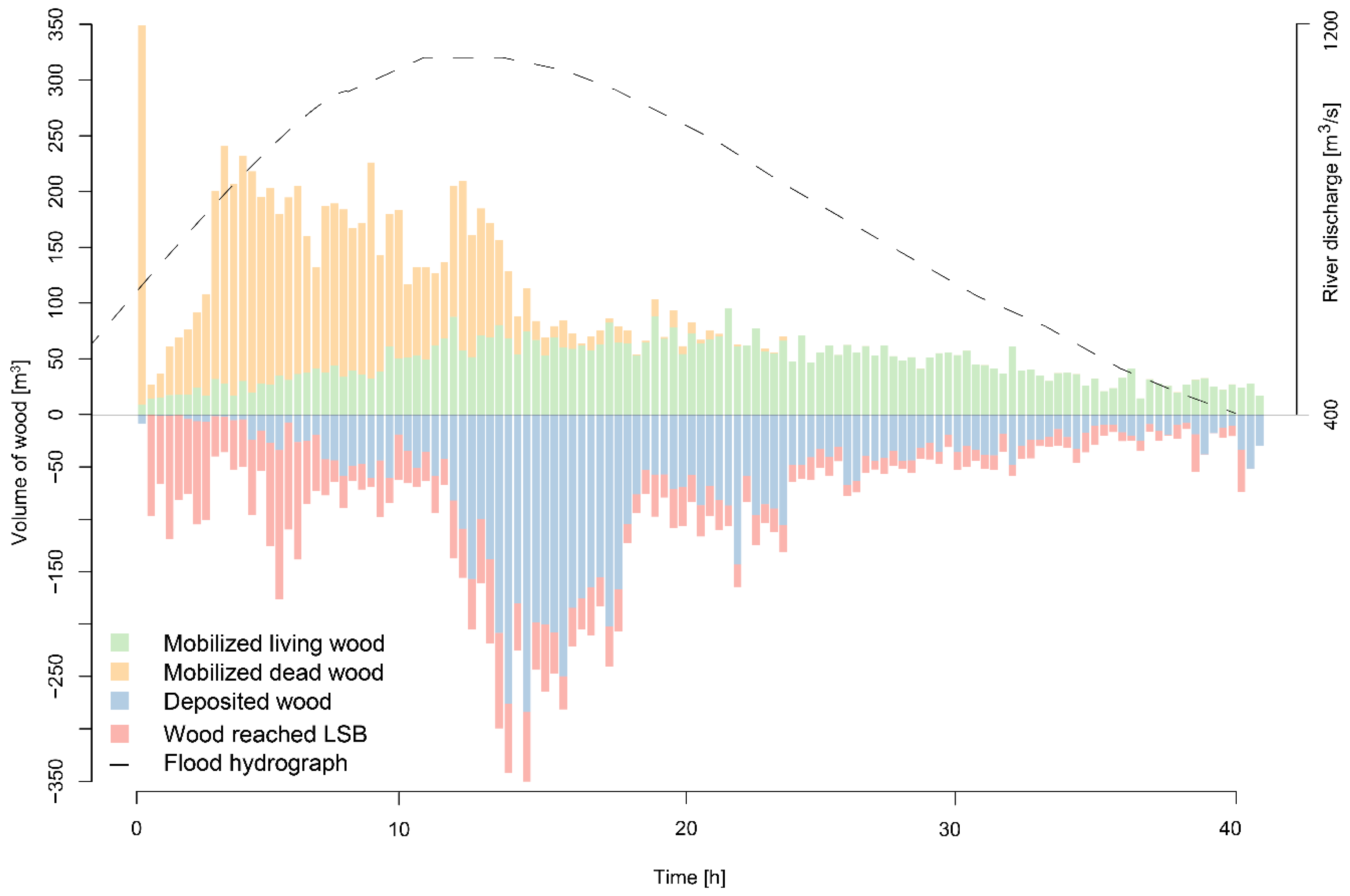
| Total mobilized wood | 11,841 |
| Mobilized in Zulg tributary | 343 |
| Mobilized living wood | 5732 |
| Mobilized deadwood | 6109 |
| Deposited after mobilization | 7288 |
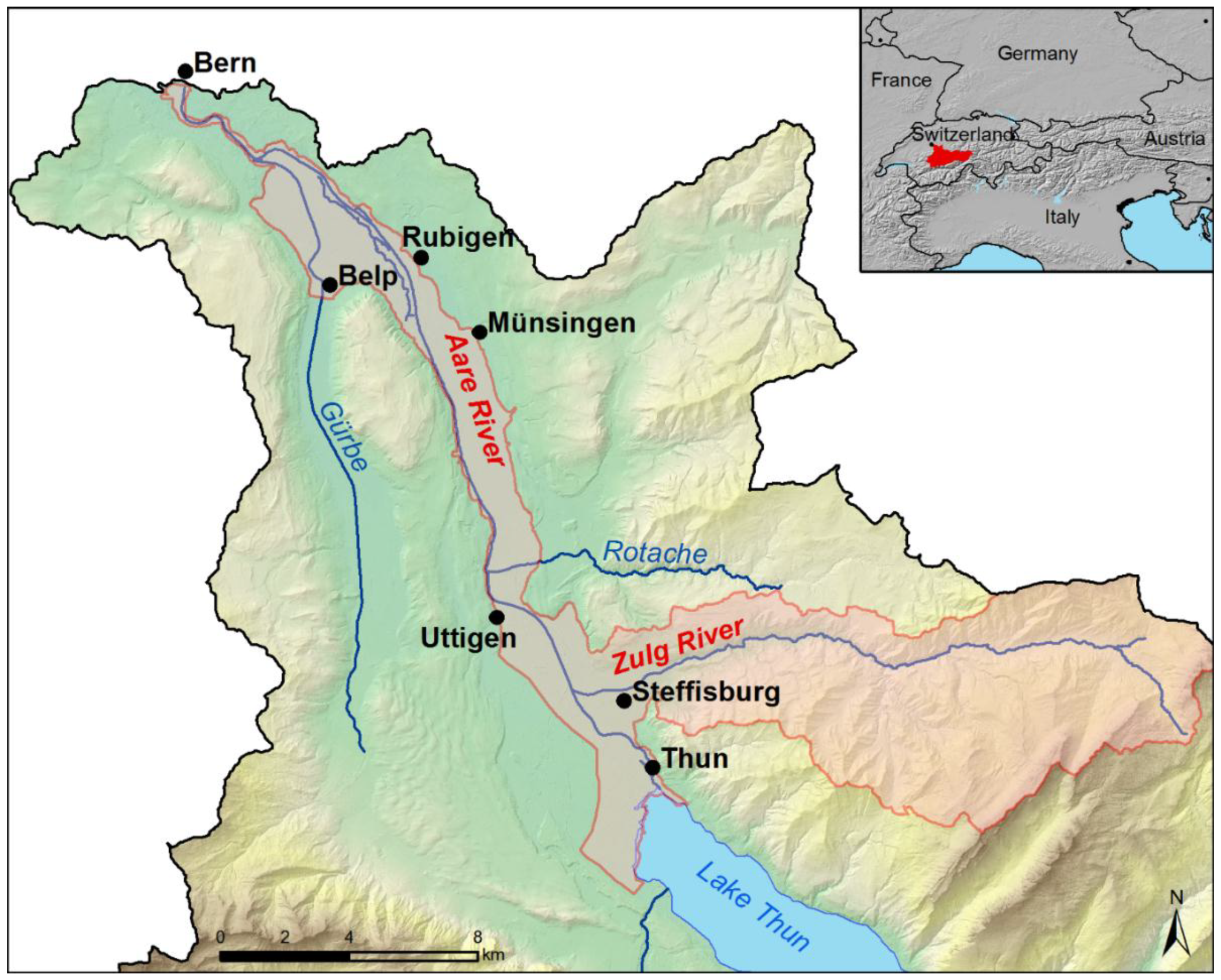
| Volume passing the lower system boundary in Bern | 3933 |
© 2018 by the authors. Licensee MDPI, Basel, Switzerland. This article is an open access article distributed under the terms and conditions of the Creative Commons Attribution (CC BY) license (http://creativecommons.org/licenses/by/4.0/).
Share and Cite
Zischg, A.P.; Galatioto, N.; Deplazes, S.; Weingartner, R.; Mazzorana, B. Modelling Spatiotemporal Dynamics of Large Wood Recruitment, Transport, and Deposition at the River Reach Scale during Extreme Floods. Water 2018, 10, 1134. https://doi.org/10.3390/w10091134
Zischg AP, Galatioto N, Deplazes S, Weingartner R, Mazzorana B. Modelling Spatiotemporal Dynamics of Large Wood Recruitment, Transport, and Deposition at the River Reach Scale during Extreme Floods. Water. 2018; 10(9):1134. https://doi.org/10.3390/w10091134
Chicago/Turabian StyleZischg, Andreas Paul, Niccolo Galatioto, Silvana Deplazes, Rolf Weingartner, and Bruno Mazzorana. 2018. "Modelling Spatiotemporal Dynamics of Large Wood Recruitment, Transport, and Deposition at the River Reach Scale during Extreme Floods" Water 10, no. 9: 1134. https://doi.org/10.3390/w10091134