Drivers of Ecosystem Metabolism in Two Managed Shallow Lakes with Different Salinity and Trophic Conditions: The Sauce Grande and La Salada Lakes (Argentina)

Abstract

Understanding the drivers and how they affect ecosystem metabolism is essential for developing effective management policy and plans. In this study, net ecosystem production (NEP), ecosystem respiration (R), and gross primary production (GPP) rates were estimated in relation to physicochemical, hydrological, and meteorological variables in La Salada (LS) and Sauce Grande (SG), two shallow lakes located in an important agricultural region with water management. LS is a mesosaline, mesotrophic-eutrophic lake, whereas SG is a hyposaline and eutrophic lake. GPP and R showed daily and seasonal variations, with R exceeding GPP during most of the study period in both lakes. Net heterotrophic conditions prevailed during the study period (NEP LS: −1.1 mmol O₂ m⁻² day⁻¹ and NEP SG: −1.25 mmol O₂ m⁻² day⁻¹). From data analysis, the temperature, wind speed, and lake volume are the main drivers of ecosystem metabolism for both lakes. Despite the significant differences between the two lakes, the NEP values were similar. The different hydrological characteristics (endorheic vs. flushing lake) were crucial in explaining why the two different systems presented similar ecosystem metabolic rates, emphasizing the importance of water management.

1. Introduction

The measurement of ecosystem metabolism with the diel oxygen technique is a reliable method to provide a measure of the overall trophic processes of an ecosystem. Primary production and respiration are the major metabolic pathways by which organic matter is produced and decomposed, respectively. Gross primary production (GPP) entails the fixation of inorganic C by photosynthesis, whereas community respiration (R) is the remineralization of the organic C to CO₂ by the organisms within an ecosystem. Therefore, the net ecosystem production (NEP) is the balance between GPP and R [1]. When NEP is greater than zero, the system is characterized as net autotrophic, supporting and exporting organic material and/or accumulating it within the system. When NEP values are below zero, it is characterized as net heterotrophic; therefore, R is subsidized by the allochthonous material [2]. This method has been applied worldwide in different types of aquatic systems, from shallow to deep lakes, most of them located in the Northern Hemisphere [3,4,5,6,7,8,9].

The metabolic rates varied across aquatic systems according to several factors. Those with high total phosphorous (TP), high chlorophyll a (Chl a), and low dissolved organic carbon (DOC) concentrations are typically characterized as autotrophic, whereas those with low TP, low Chl a, and high DOC concentrations are characterized as heterotrophic [4,10]. Moreover, the concentrations of these parameters can change in lakes according to the water management and catchment use conditions. Those lakes located in agrarian landscapes are particularly affected by nutrient loading from the catchment [11] leading to eutrophication [12]. Previous studies in La Salada (LS) found that water input changes the nutrient and salinity concentrations, and produces substantial changes in the composition and biomass of the planktonic community [13]. Also, an important source of additional energy to R is the input of allochthonous organic matter via streams [14,15,16]. According to [5], a lake´s morphometry and catchment conditions are crucial to determining the human impact on ecosystem metabolism. They found that with greater lake area, water depth, and drainage, the ratio of GPP and R decreased. Also, these authors found that small lakes with less incident light were characterized by NEP < 0 conditions, and finally that daily variations in GPP decreased with the lake area and water depth due to the effect of lower nutrient input per volume unit. On the other hand, the meteorological conditions also regulate GPP and R rates within a lake. It was found that wind or precipitation events (storms) produced changes in GPP and R rates, decoupling both variables temporarily which later returned to the previous conditions [9].

Finally with respect to their morphology, shallow lakes, which represent the most abundant lake type in the world [17] show different functional behavior with respect to deep ones [18,19]. Those located in the Pampean region (Argentina) are mostly shallow and polymictic, ranging from eutrophic to highly hypertrophic [20]. The precipitation, evaporation cycles, and water management have an important influence on water renewal time and salinity, which are highly variable [13,21,22]. In particular, the water level fluctuations coupled with salinity increments could change the trophic structure as the species diversity declines when their osmotic tolerance is exceeded [23,24,25,26]. Moreover, the structure of aquatic communities in saline lakes could change significantly with other factors, such as habitat permanence, water management, inflows of fresh water, and trophic interactions [27,28,29,30]. The alternative stable states theory [31] proposes that lakes can be in two alternative stable states: clear with abundant submerged macrophytes or turbid with few submerged plants, both well represented on the Pampas plain [32].

In conclusion, there is a wide mixture of stressors affecting lakes, and understanding how these drivers affect the ecological status through the study of the ecosystem metabolism resulted in a valuable tool for the development of effective management policy and plans. La Salada (LS) is an endorreic, mesosaline, mesotrophic to eutrophic lake that has been studied in recent years for its ecosystem metabolism [7], plankton community [13], and ecosystem services [33]. Sauce Grande (SG) is a flushing, hyposaline, and eutrophic lake that has been studied for its hydrology [34], water quality [35], and plankton community [36,37]. Therefore, we hypothesized that (1) water management will influence ecosystem metabolism with the increment of GPP and R rates through nutrients, DOC, and organic matter loadings from the catchment in both lakes, and (2) that the different salinity, trophic status, and hydrological functioning will result in contrasting metabolism conditions for both lakes.

2. Materials and Methods

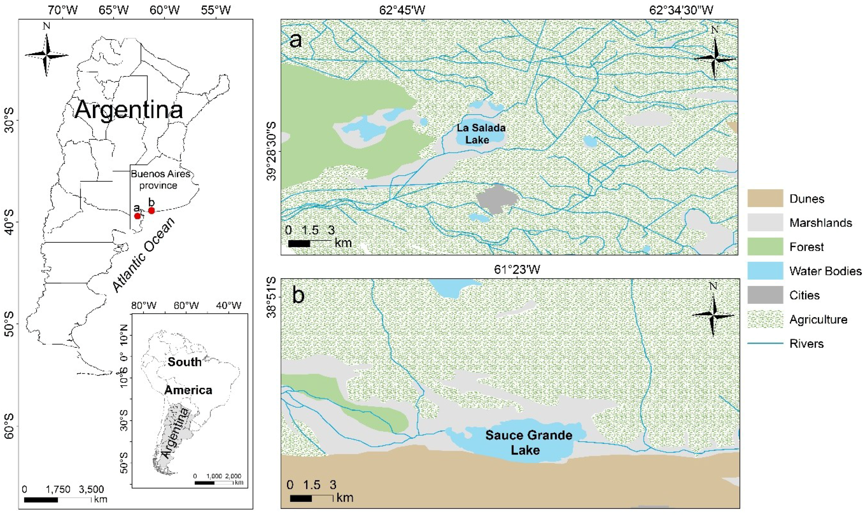
This study includes the physicochemical and hydrological surveys over two years for two shallow lakes: from January 2014 to December 2014 for the La Salada lake and from September 2016 to October 2017 for the Sauce Grande lake. The surveys included both low-frequency sampling and high-frequency data obtained with an instrumented buoy located in the deepest part of each lake.

2.1. Study Sites

La Salada (39°27′ S, 62°42′ W) is a shallow saline lake situated in the south west of the Pampean region (Argentina) (Figure 1a). It is a small polymictic lake (4 km²) with a mean depth of 2.5 m. Its main affluent is a channel derived from the Colorado river, which is managed by the Development Corporation of the Colorado River Valley ((Production Development Corporation) CORFO in Spanish), which decides when and how much water enters the lake. The irrigation system gates are open each year from 1 August to 1 May. It is a small circular lake, with the presence of some reeds in the margins of the channels. It is an alkaline, mesotrophic-eutrophic lake, with a low average concentration of Chl a (8.6 µg L⁻¹), and the bottom presents a dense cover of charophytes in most of the central part [38]. The presence of the omnivorous fish Odonthestes sp. is common in this lake, considered of great importance for sport fishing and consequently for tourism [39].

The SG lake (38°57′ S, 61°24′ W) is located in the south east of the Pampean region (Argentina) (Figure 1b). It is a natural water body with a surface area of 15.87 km² and a mean depth of 1.1 m [40]. It is a flushing lake with an affluent, the Sauce Grande River, and a connection with the Atlantic Ocean. The water flow of its affluent is managed by the Paso de las Piedras Dam, which supplies water to the cities of Bahía Blanca and Punta Alta. Water is released downstream only when the dam is full [41]. The SG lake is polymictic, rich in dissolved oxygen, turbid, and eutrophic, with an average concentration of Chl a of 171 µg L⁻¹ [37,39]. It is a large and elongated depression, with low coasts with smooth slopes (usually muddy and with reeds on the northern side), while a coastal dune system controls the southern coast. The bottom is almost entirely mud. The presence of the fish Odontesthes sp. is also frequent in this lake [42].

The climate in the area of LS is cold temperate and mostly dry, whereas in the SG area it is temperate [43]. Annual air temperature values are between 14 and 20 °C, with pronounced summers and winters. Wet and dry cycles characterize the Pampean region. The highest precipitation occurs typically in spring and summer, with an average annual rainfall of 692 mm for the SG area and 369 mm for the LS area [43]. Prevailing winds in the region are from the north west, with a mean speed between 3.9 and 4.1 m s⁻¹ [43].

2.2. Environmental Variables, Land Use, and Hydrological Conditions

For nutrient concentrations analysis, monthly samples of water were taken with a van Dorn bottle at 0.5 m depth and filtered through Whatman GF/F filters (Merck KGaA, Darmstadt, Germany). Total phosphorus was estimated with acid digestion with potassium persulfate (120 °C for 1 h) following [44]. Total organic nitrogen (TNorg) was determined by the semi-micro Kjeldahl method [44].

Suspended particulate matter (SPM) was determined by weighing the residue resulting from the filtration through a GF/F filter according to [44]. Chl a concentration was estimated with a fluorometer (SLM instruments, Urbana, IL, USA), using 90% acetone as the extraction solvent [45]. Water transparency was estimated with a Secchi disk. Trophic status was assessed with Carlson´s trophic index from TP, Chl a, and Secchi disk values [46]. Historical precipitation values were obtained from two meteorological stations, one located 10 km from LS, National Institute of Agricultural Technology in Hilario Ascasubi (INTA in Spanish) [47], and the other located at 23 km from SG, INTA Coronel Dorrego [47] to assess the effect of rainfall on physicochemical values and metabolism rates. To classify the intensity of dry and wet conditions the standardized precipitation index (SPI) was calculated, which quantifies the precipitation anomalies [48]. Finally, the water input for each lake was obtained from CORFO in the case of LS and from measurements of the discharge in the Sauce Grande River with a Sontek^® Acoustic Doppler Profiler (ADP) (San Diego, CA, USA) based on the River Surveyor system (SonTek, San Diego, CA, USA). The system is mounted on a vessel to collect the data used to make an instantaneous measurement of river discharge. The ADP measures the water current velocity simultaneously at multiple depth locations through the water column and over most of the cross-section of the river. This velocity field then was combined with the bathymetry of the section to measure instantaneous discharge, and then the River Surveyor program computed the total discharge.

2.3. Bathymetry

The bathymetry was performed by an autonomous unmanned vehicle (drone for bathymetry) based on Arduino, open electronic platform, developed at the Argentine Institute of Oceanography. The vehicle is fitted out with an autopilot system and echo sounder using a Garmin Echo 150 transducer that operates at 200 kHz and with water quality sensors. The route was followed using the Mission Planner software [49]. The echo sounder system is integrated with Mission Planner to monitor the echo sounder profile during the field work. All the data are saved on a memory card on board (GPS, acoustic profile and navigation parameters). A GNU Octave script was written to process all the data recorded from the drone. The coastline was determined using Landsat 8 images according to fieldwork dates. The Landsat images were processed using the software ArcGIS^® 10.2.2 software (Environmental Systems Research Institute, Redlands, CA, USA). Finally, a linear triangulation interpolation method was used to estimate the bathymetry from the depth values (from the GNU Octave script) and the coastline points (zero level).

2.4. Estimation of Metabolism

Meteorological and water variables were measured at 10-min intervals from two buoys (Estación de Monitoreo Ambiental Costero, EMAC) moored approximately in the deepest point of each lake (Figure 2). The physicochemical variables were measured at a 0.5-m depth, including dissolved oxygen (DO), water temperature, water level and electrical conductivity. Meteorological variables were measured at 2.10 m in height on the buoy, including air temperature and wind speed and direction. Data is available on the website www.emac.iado-conicet.gob.ar [50].

Estimation of the ecosystem metabolism was based on [1], with modifications for saline environments for LS and high wind environments for both lakes [51]. Hourly NEP (NEP_h) (mmol O₂ m⁻³ h⁻¹) was calculated as the difference between the changes in DO concentration (∆DO) and the fraction between the diffusive oxygen exchange of gas with the atmosphere (F) and the daily mean water depth (z) (

Table 1. Equations for the estimation of ecosystem metabolism in the La Salada (LS) and Sauce Grande (SG) lakes during the study period. NEP: net ecosystem production; GPP: gross primary production; R: ecosystem respiration.

Variable	Equation
Hourly NEP	$NE{P}_h=\Delta DO-\frac{F}{z}$
Diffusive oxygen exchange	$F=k\left(DO-D{O}_{sat}\right)$
Coefficient of oxygen exchange	$k=k_{660}{\left(\frac{Sc}{660}\right)}^{\frac{1}{2}}$
Schmidt number for LS	$S_c=1953.4 - 128.0 T + 3.9918 T^2 - 0.046527 T^3$
Schmidt number for SG	$S_c=1800.6-120.1 T+3.7818 T^2-0.0476 T^3$
Gas piston velocity	$k_{660}=\left(2.07+0.215 U_{10}^{1.7}\right)/100$
Wind speed at 10 m	$U_{10}=a U_{2.1}$
Correction factor	$a=1.4125h^{-0.15}$
NEP during daytime	$NE{P}_{daytime}=mean NEP during daylight\times dayfraction\times 24 h$
R during daytime	$R_{daytime}=R_{hr}\times 24 h\times dayfraction$
R	$R_{day}=R_{hr}\times 24 h$
NEP	$NEP=GPP-R_{day}$
GPP	$GPP=NE{P}_{daytime}+R_{daytime}$

). Unlike stratified lakes, we employed the daily mean depth instead of the mixing depth as both lakes are polymictic considering their shallow depth, the flat shape of the basins, and freedom from obstacles and continuous wind action [21,22,52]. F (mmol O₂ m⁻³ h⁻¹) was calculated as the difference between the DO measured and the concentration of oxygen in equilibrium with the atmosphere (DO_sat), where k is the coefficient of oxygen exchange at a given temperature (Table 1). This was computed from the Schmidt number (Sc) and the gas piston velocity (k₆₆₀), with a correction for high wind environments, using a half coefficient instead of two-thirds [51]. In this study, the Sc was calculated at each time step using the DO-specific equation of [53], but using the coefficients for seawater for the LS lake (4) and freshwater for the SG lake (5) (Table 1). The k₆₆₀ was estimated with a correction for high wind environments based on the equation proposed by [54] as a function of wind speed at 10 m above the lake surface (U₁₀). As the wind speed at the buoy is measured at 2.10 m above the water (U_2.1), U₁₀ was calculated assuming a neutrally stable boundary layer from the relationship given by [55] and a is a correction factor (Table 1).

To obtain GPP, R, and NEP values, NEP occurring during photosynthesis (NEP_daytime) was estimated as the mean hourly NEP taking place between sunrise and sunset extrapolated over day length [2]. The fraction of the day when there was daylight (day fraction) was calculated from latitude and date of measurements in radians (Table 1). We assume that there is no photosynthesis at night and GPP = 0 (therefore R = NEP during the nighttime), and that R during nighttime was equal to R during the daytime. Hourly respiration rates derived from changes in DO concentration during nighttime (R_hr) were extrapolated over a 24-h period to calculate the respiration during the day (R_day). Respiration during the daytime (R_daytime) was calculated from mean NEP_hr during darkness (R_hr) extrapolated over a day length. Finally, as NEP during daytime is the difference between GPP and R_daytime, GPP was calculated as the NEP_daytime added to R_daytime (Table 1). All rates were integrated daily (day⁻¹).

2.5. Statistical Analysis

Relationships between weekly metabolic rates and environmental variables were analyzed using correlation coefficients (Pearson) with appropriate software. Normality was examined through the Kolmogorov–Smirnov test [56]. High-frequency data was analyzed spectrally using fast Fourier transform to define any potential periodicity of the variables [57]. Furthermore, a multiple regression analysis was performed with daily environmental and metabolic data to explain the variation in metabolic rates with respect to the most significant environmental variables.

3. Results

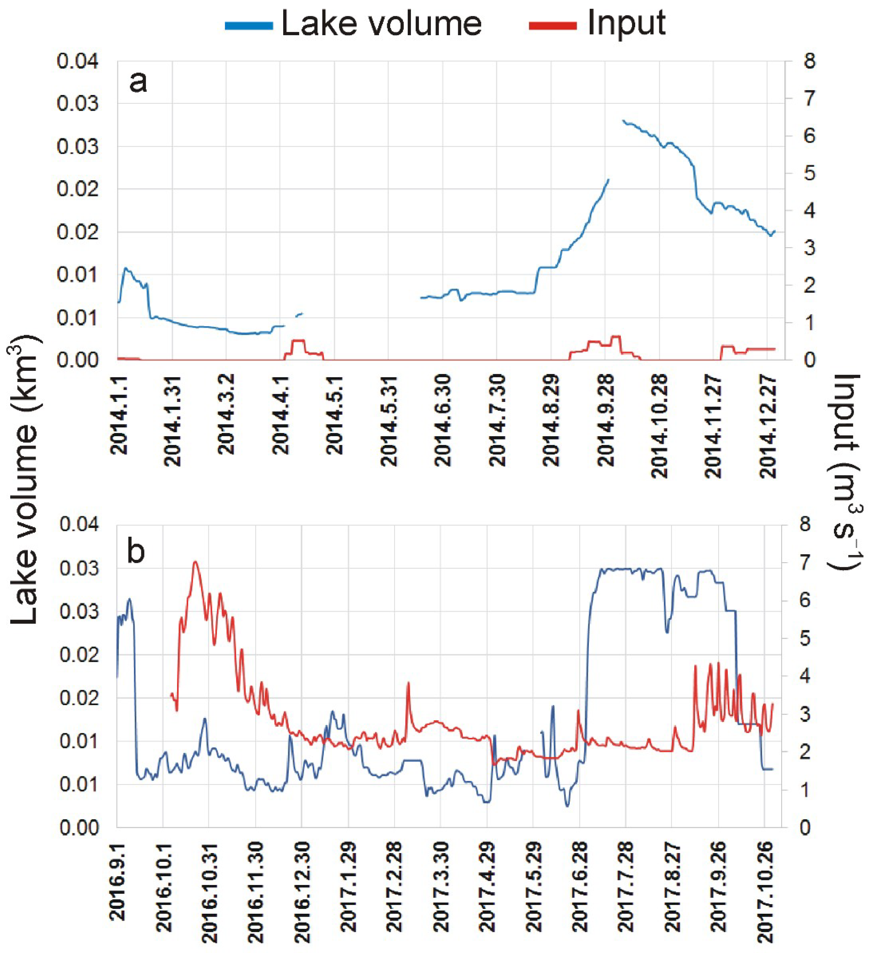
3.1. Environmental Variables, Land Use, and Hydrological Conditions

LS was characterized by a mesotrophic to eutrophic condition with low Chl a values. Suspended particular matter (SPM) and particulate organic matter (POM) values were also low, showing high transparency conditions during the entire study period, with a Secchi disk mean value of 1.6 m (

Table 2. Mean, standard deviation (SD), minimum (Min), and maximum (Max) values of the environmental parameters measured in La Salada and Sauce Grande Lakes during the study period. Temp: water temperature; Cond: conductivity; Level: water level; Prec: precipitation; Vol: lake volume; DO: dissolved oxygen; Chl a: chlorophyll a; SPM: suspended particulate matter; POM: particulate organic matter; TP: total phosphorous; TNorg: total organic nitrogen.

Variables	Sauce Grande				La Salada
	Mean	SD	Min	Max	Mean	SD	Min	Max
Temp (°C)	17.1	6.5	12.1	24.5	16.0	5.7	7.5	25.2
Cond (mS cm−1)	2.5	0.2	2.3	2.8	49.9	4.7	41.6	58.0
Level (m)	1.7	0.2	1.3	2.1	2.3	0.3	2.1	3.20
Caudal (m3 s−1)	2.8	1.1	1.7	7.0	0.28	0.16	0.03	0.64
Wind (m s−1)	3.3	2.6	0.0	13.2	6.6	4.3	0.0	27.6
Prec (mm)	33.8	12.0	18.9	49.2	52.2	29.5	8.0	92.5
Vol (km3)	0.013	0.009	0.003	0.030	0.012	0.008	0.003	0.028
pH	10.0	0.4	9.7	10.4	8.1	0.4	7.1	8.6
DO (mg L−1)	5.9	1.3	4.9	7.4	9.8	2.0	6.5	12.2
Chl a (µg L−1)	59.6	36.6	20.9	93.7	9.0	5.0	3.1	15.6
SPM (mg L−1)	64.8	14.6	50.8	80.0	40.9	25.2	6.4	100.4
POM (mg L−1)	33.4	16.9	20.0	52.5	12.3	21.5	2.4	76.9
Secchi disk (m)	0.28	0.7	0.20	0.33	1.6	0.7	0.0	2.7
TP (mg L−1)	0.1	0.09	0.04	0.21	0.05	0.02	0.03	0.09
TNorg (mg L−1)	12.8	4.7	9.4	18.2	3.5	0.2	3.3	3.8

) and a mean euphotic zone value of 4.3 ± 1.9 m. LS is a lake rich in DO with alkaline conditions (Table 2). Nutrient concentrations were also high during the entire study period (Table 2). With respect to land use, 74.8% of the lake’s area of influence (220 km²) was represented by agricultural systems, 12.1% by forests, 8.2% by marshlands, and 1.4% by human settlements. According to SPI values, 2014 was a year with wet conditions. The lake experienced great changes during the study period associated with the water inflow and the consequent water level fluctuations (Figure 3). The mean lake volume during the study period was 0.0117 ± 0.0075 km³ (Figure 3a). During 2014, the total amount of water that entered the lake was 0.0025 km³, reaching a maximum of 0.00005 km³ day⁻¹ during October 2014. The water volume varied in response to the water input (Figure 3a). The maximum water level values were recorded in October 2014 and the minimum during February 2014 (Table 2). Conductivity was high, classifying LS as a mesosaline lake. Depending on the water level fluctuations, the conductivity values presented minimum values during October 2014 and maximum during March 2014. Precipitation values presented minimum values in January 2014 and maximum in March 2014 (Table 1).

The SG Lake presented eutrophic conditions during the entire study period. In contrast with LS, it presented higher Chl a, nutrient, MPS, and MOP values (Table 2). Transparency was low with a Secchi disk mean value of 0.28 m and a mean euphotic zone value of 0.7 ± 0.2 m. Thus, it was classified as an alkaline lake, rich in DO. With respect to the nutrient concentrations, TP was twice that in LS, and TNorg was three times the concentration value. With respect to the land use in the area of influence of the lake (780 km²), 62% of the area is devoted to agricultural systems, 22.9% to dunes, 9.8% to marshlands, 1.7% to forests, and only 0.5% to human settlements. SPI values characterized the study period as normal conditions. In contrast with LS, volume fluctuations during the study period were not clearly associated with the water inputs (Figure 3b). The mean lake volume was 0.013 ± 0.0095 km³, with maximum values during the spring of 2017. During the study period, the total amount of water that entered the lake was 0.095 km³ (Figure 3b), reaching a maximum of 0.00061 km³ day⁻¹ during October 2016. Conductivity was low, classifying SG as a hyposaline lake (Table 2). Minimum values were recorded in March 2017 and maximum in April 2017. Precipitation values presented minimum values in July 2017 and maximum values in February 2017 (Table 2).

3.2. Lake Metabolism

In the LS Lake, GPP and R showed daily and seasonal variations, with R exceeding GPP during most of the study period (Figure 4). The mean monthly R value (17.21 mmol O₂ m⁻³ day⁻¹) slightly exceeded the mean monthly GPP value (16.61 mmol O₂ m⁻³ day⁻¹) (Figure 4d) presenting a GPP/R ratio of 0.91. Monthly GPP ranged between 6.32 mmol O₂ m⁻³ in June 2014, and 29.1 mmol O₂ m⁻³ day⁻¹ in January 2014. GPP presented a seasonal pattern increasing during summer and spring and decreasing during autumn and winter (Figure 4a,d). Temporal variation in R presented a similar pattern and was positively correlated with GPP (Figure 5). The minimum monthly R value was 8.35 O₂ m⁻³ day⁻¹ during June 2014 and the maximum value was 30.8 O₂ m⁻³ day⁻¹ in January 2014 (Figure 4b,d). NEP monthly values varied between −7.0 O₂ m⁻³ day⁻¹ during April 2014 and 3.5 O₂ m⁻³ day⁻¹ during December 2014. NEP < 0 occurred during most of the study period except during spring of 2014 (Figure 4c,d). Mean monthly NEP value was −1.1 O₂ m⁻³ day⁻¹ classifying LS as a heterotrophic lake during the study period. Fourier analysis showed maximum densities on monthly, 11-day and weekly scales, and minor scales at 3 days for the three metabolic variables. With regard to the environmental variables, the water input, water temperature, wind speed, and conductivity coincide with these scales, whereas the water volume only showed maximum densities on the monthly scale.

In SG lake GPP and R also showed daily, and seasonal variations, with R showing greater or similar values with respect to GPP (Figure 4). The mean R value was 13.9 O₂ m⁻³ day⁻¹, and the mean GPP value was 12.6 O₂ m⁻³ day⁻¹ presenting a GPP/R ratio of 0.93. Monthly GPP ranged between 8.1 O₂ m⁻³ day⁻¹ during October 2016 and 21.2 O₂ m⁻³ day⁻¹ during March 2017 (Figure 4h). GPP showed a seasonal pattern with maximum values during summer of 2017, decreasing towards colder months. R presented a similar seasonal pattern (Figure 4f,h) with minimum values during October 2016 (7.2 O₂ m⁻³ day⁻¹) and maximum during March 2017 (25.8 O₂ m⁻³ day⁻¹). Both variables were positively correlated (Figure 5). The NEP mean value during the study period was −1.25 O₂ m⁻³ day⁻¹, with NEP < 0 during most of the study period, classifying SG as a heterotrophic lake (Figure 4g,h). Minimum NEP values were recorded during March 2017 (−4.1 O₂ m⁻³ day⁻¹) and maximum during October 2017 (0.9 O₂ m⁻³ day⁻¹) (Figure 4h). Fourier analysis showed maximum densities on monthly, 11-day and weekly scales and minor scales at 3 days for the three metabolic variables. These coincide with the maximum densities found in the water input, DO, wind speed, and water temperature, whereas the lake volume only presented maximum values on the monthly scale and conductivity on the monthly and 10-day scales.

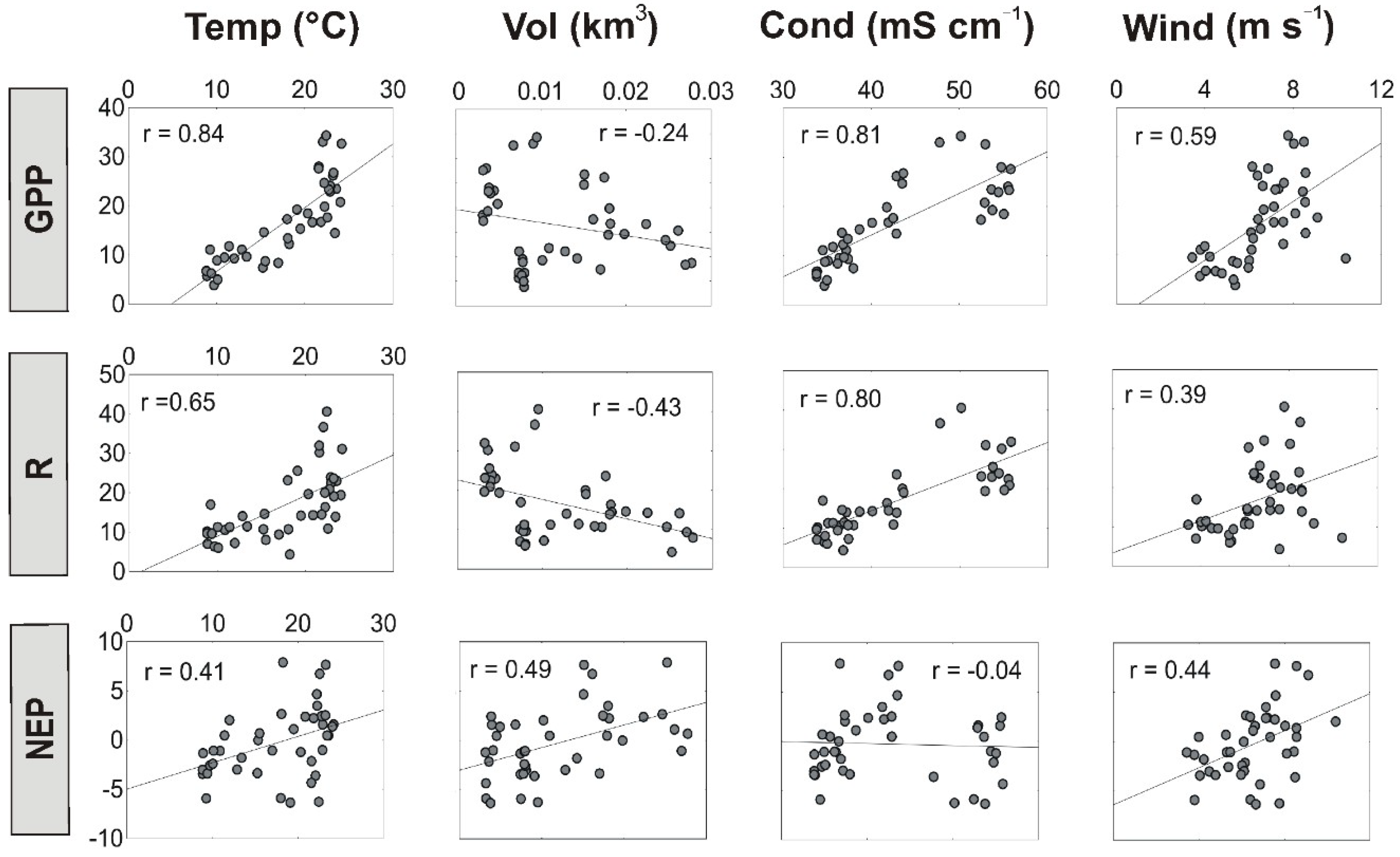
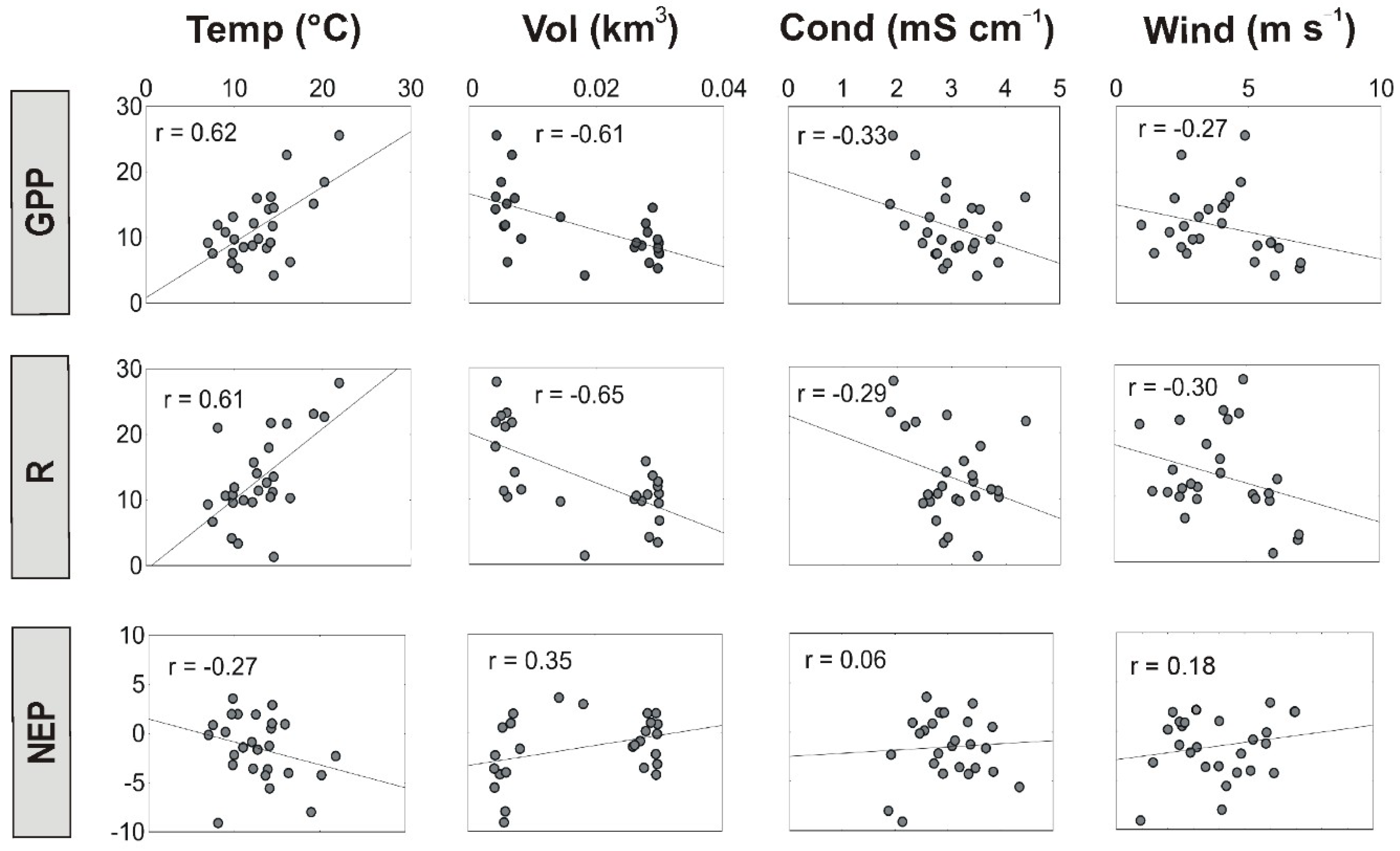
3.3. Regulation of Lake Metabolism

With respect to the average weekly metabolism rates, in LS lake GPP, R, and NEP were positively correlated with water temperature and wind speed during the study period. Moreover, R and GPP were also positively correlated with the conductivity. Finally, R was negatively correlated with lake volume, and NEP was positively correlated (Figure 5). In the case of SG lake, GPP and R were positively correlated with water temperature and negatively correlated with lake volume, whereas NEP was positively correlated (Figure 6). The environmental variables measured monthly (e.g., TP, TNorg, Chl a, etc.) were not included in the statistical analysis because of the small number of measurements. From multiple regression analyses the variables that best described the metabolism rates from the daily measurements were the water temperature, wind speed, and lake volume for both lakes (

Table 3. Multiple regression analysis for GPP: Gross primary production, R: community respiration, and NEP: net ecosystem production as a function of Temp: water temperature (°C), Wind: wind speed (m s⁻¹) and Vol: lake volume (m³ seg⁻¹) in the La Salada and Sauce Grande lakes during the study periods.

Lake	Dependent Variable	Parameter	R2	Standarized Regression Coefficient	t	P
La Salada	GPP	Temp	0.392	0.51	1.32	<0.0001
		Wind		0.50	−0.12	<0.0001
		Vol		−1.50	−294.61	<0.0001
	R	Temp	0.299	0.50	1.09	<0.0001
		Wind		0.49	−0.19	<0.0001
		Vol		−1.50	−507.73	<0.0001
	NEP	Temp	0.362	0.50	2.42	<0.0001
		Wind		0.50	−0.29	<0.0001
		Vol		−1.50	−831.22	<0.0001
Sauce Grande	GPP	Temp	0.255	0.4	0.91	<0.0001
		Wind		−0.09	−0.68	<0.0001
		Vol		−1.34	−4.80	<0.0001
	R	Temp	0.302	1.1	1.29	<0.0001
		Wind		−0.72	−0.57	<0.0001
		Vol		0.57	0.74	<0.0001
	NEP	Temp	0.314	−0.35	2.30	<0.0001
		Wind		−0.57	−1.14	<0.0001
		Vol		1.49	31.14	<0.0001

).

4. Discussion

Rates of ecosystem metabolism obtained in both lakes showed large variations on a daily basis and across seasons during the study period. The general annual balance characterized both shallow lakes as heterotrophic. With respect to other studies that have dealt with ecosystem metabolism, only a few were carried out in shallow saline systems and at low frequency [7,58,59]. Moreover, most of them were in the Northern Hemisphere and only for the few months when they were iceless (e.g., [6]) and not over the entire year as in this study. If LS and SG NEP rates are compared with other shallow lakes, most of them showed higher negative [2,10,59,60,61] or positive NEP values [6,10,59,62]. However, most of the other data referred to periods of only a few months, usually over the summer, when productivity was greatest. In this study the net heterotrophic conditions found contradict the expected NEP > 0 values according to their nutrient and Chl a concentrations [4,10], but again, these studies are based on the analysis of a short period and may differ in comparison with the estimations of ecosystem metabolism based on an entire year.

Daily GPP and R were closely linked during the entire study period. This is consistent with the positive correlation founded between GPP and R, and the monthly NEP values near zero during most of the study period. According to [1] this could be explained by the relatively rapid respiration by bacteria and zooplankton of the newly produced organic matter within the lakes. This could be the case in both lakes as high abundances of zooplankton for LS (up to 1300 ind L⁻¹), bacteria (up to log₁₀ 3.89 colony formation units (CFU)), and mesozooplankton (up to 100 ind L⁻¹) for SG are cited in previous studies [13,35,37]. In other studies, GPP and R were are also coupled and positively correlated as in this case [6,8,16]. Nevertheless, it was documented that the presence of high winds or unusual precipitation events could temporarily produce decoupling between these two variables [9,63,64]. However, although LS and SG are characterized by the presence of high winds [43], neither of the lakes showed this kind of disruption.

According to the temporal pattern for metabolic rates in both lakes, maximum values for GPP and R were found during warmer months and minimum values towards colder months. This was reflected in the positive correlations of the metabolic rates with water temperature. This is in agreement with the results cited for other shallow lakes where seasonal patterns are the result of variations in light and temperature [2,6,7,16,61]. As well as the water temperature, most of the processes were influenced by lake volume for both lakes, and wind speed and conductivity for LS. In other studies, wind speed presented a negative relationship with GPP and NEP values associated with turbidity conditions [6]. Nevertheless, in LS, it was positively related to the metabolic rates because, unlike other shallow lakes, LS has charophytes on the bottom that prevent the resuspension of sediments with major wind speed. Finally, the use of lake volume instead of water level, as in other studies [6,61], resulted in better comparisons between the morphologically different lakes as in this case. SG presented a greater area than LS, but the lake volume was similar and so they were comparable. In this study, the lake volume was negatively correlated with GPP and R, as in other studies, and could be attributed to the dilution of organisms and nutrients within the lake [61].

The annual GPP/R ratio in both lakes was near one, indicating that the main substrate for R is the GPP within the lake; nevertheless, the fact that NEP < 0 determines that this would be insufficient. Possibly, the origin of organic resources respired during heterotrophy conditions might arise either from the excess of GPP generated when the system is under autotrophic conditions or from the allochthonous material. The allochthonous input of organic matter via streams is an important source of supplementary energy for the community R [14,16]. Besides, both lakes are located in important agricultural areas where fertilization of crops with nitrogen is a common practice applied from June to July (seedtime) and from September to October (tillering) [65]. In a previous study in LS an increment in GPP and R values was observed after water input [7], and an increase in nutrient concentrations and a decrease in conductivity, leading to changes in plankton composition and biomass [13]. In this study, an increase in GPP and R values was also observed in LS, accompanied with the maximum increase in its volume. Considering that the water comes from the irrigation of crops, this finding suggests that the supply of nutrients, new organic material, and/or plankton organisms from the river would promote GPP and R, respectively. According to [5], the input of DOC and nutrients increases with a high drainage ratio (catchment area to lake surface area). Also, small lakes possess a long shoreline relative to lake volume and receive significant inputs of organic matter [66], increasing R and leading to NEP < 0 conditions [1,10]. In the same manner, in SG, GPP, and R showed a stronger negative relation with lake volume, but NEP was positively correlated. Nevertheless, SG has a different hydrological function from LS, where greater water input was recorded, but the lake volume did not respond immediately to these variations as in LS. The explanation for this is that SG is a flushing lake and part of the input and production within the lake of DOC, nutrient and organisms are delivered to the sea. Nevertheless, the increases in nutrient concentrations coinciding with the increments in water input and lake volume could explain the positive correlation with NEP values for both lakes.

Finally, according to Scheffer’s stable states theory [31], LS is in a clear state during the whole study period and dominated by the presence of charophytes which prevent the resuspension of sediments [13], whereas SG is in a turbid state during the whole study period and dominated by phytoplankton [36,37,67]. It is well known that solar light promotes primary production (GPP) and the later the respiration processes (R) that occur within a lake ecosystem [68]. The fact that the euphotic zone is reduced in SG, unlike LS, could explain the lower GPP rates and explain why it presented a stronger negative relation with lake volume. Meanwhile in LS, GPP was weakly related to lake volume because charophytes (and phytoplankton as well) receive light during the whole year, independently of the significant water level fluctuations. In a study of 25 Danish lakes with alkaline and nutrient-rich catchments and relatively low transparency conditions [5], it was found that the benthic zone was dominated by sediments rich in carbon, with a high demand of oxygen. This suggests the dominance of heterotrophic processes, which is in accordance with the case of SG. Furthermore, according to a study performed in two eutrophic lakes with similar nutrient concentrations, they found that the one with submerged plants presented substantially higher GPP rates than the one that only had phytoplankton and periphyton [69]. In this study, LS presents submerged charophytes, and the GPP rates were greater than in SG. Furthermore, if salinity conditions are considered, LS is a mesosaline lake. Increased salinity could result in ion toxicity and osmotic stress accompanied by high mortality or lower reproduction and growth rates for salt-sensitive taxa [70,71]. Therefore, it would be expected that these conditions are limiting GPP in comparison with SG.

In conclusion, temperature resulted the main driver of ecosystem metabolism for both lakes, but the NEP values resulted similar during this study, in contrast to what was expected from the different salinity, trophic status, and hydrology conditions. The high transparency conditions of LS allowed the presence of macrophytes. This was in conjunction with the endorreic condition and the fact that water input promoted increases in GPP and R. In contrast, the flushing and turbid conditions in SG promoted decreases in GPP and R rates under lower volume conditions. These findings emphasize the importance of water management in lakes found in agricultural systems.

References

1. Staehr, P.A.; Bade, D.; Van de Bogert, M.C.; Koch, G.R.; Williamson, C.; Hanson, P.; Kratz, T. Lake metabolism and the diel oxygen technique: State of the science. Limnol. Oceanogr. Methods. 2010, 8, 628–644. [Google Scholar] [CrossRef] [Green Version]
2. Cole, J.J.; Pace, M.L.; Carpenter, S.R.; Kitchell, J.F. Persistence of net heterotrophy in lakes during nutrient addition and food web manipulation. Limnol. Oceanogr. 2000, 45, 1718–1730. [Google Scholar] [CrossRef]
3. Lauster, G.H.; Hanson, P.C.; Kratz, T.K. Gross primary production and respiration differences among a littoral and pelagic habitats in northern Wisconsin lakes. Can. J. Fish. Aquat. Sci. 2006, 63, 1130–1141. [Google Scholar] [CrossRef]
4. Sand-Jensen, K.; Staher, P.A. Scaling of pelagic metabolism to size, trophy and forest cover in small Danish lakes. Ecosystems 2007, 10, 127–141. [Google Scholar] [CrossRef]
5. Staehr, P.A.; Baastrup-Spohr, L.; Sand-Jensen, K.; Stedmon, C. Lake metabolism scales with lake morphometry and catchment conditions. Aquat. Sci. 2012, 74, 155–169. [Google Scholar] [CrossRef]
6. Laas, A.; Nõges, P.; Kõiv, T.; Nõges, T. High-frequency metabolism study in a large and shallow temperate lake reveals seasonal switching between net autotrophy and net heterotrophy. Hydrobiologia 2012, 694, 57–74. [Google Scholar] [CrossRef]
7. Alfonso, M.B.; Vitale, A.J.; Menéndez, M.C.; Perillo, V.L.; Piccolo, M.C.; Perillo, G.M.E. Estimation of ecosystem metabolism from diel oxygen technique in a saline shallow lake: La Salada (Argentina). Hydrobiologia 2015, 752, 223–237. [Google Scholar] [CrossRef]
8. Tonetta, D.; Staehr, P.A.; Schmitt, R.; Petrucio, M.M. Physical conditions driving the spatial and temporal variability in aquatic metabolism of a subtropical coastal lake. Limnologica 2016, 58, 30–40. [Google Scholar] [CrossRef]
9. Richardson, D.C.; Carey, C.C.; Bruesewitz, D.A.; Weathers, K.C. Intra-and inter-annual variability in metabolism in an oligotrophic lake. Aquat. Sci. 2017, 79, 319–333. [Google Scholar] [CrossRef]
10. Hanson, P.C.; Bade, D.L.; Carpenter, S.R. Lake metabolism: Relationships with dissolved organic carbon and phosphorus. Limnol. Oceanogr. 2003, 48, 1112–1119. [Google Scholar] [CrossRef] [Green Version]
11. Heathwaite, A.L. Multiple stressors on water availability at global to catchment scales: Understanding human impact on nutrient cycles to protect water quality and water availability in the long term. Freshwater Biol. 2010, 55, 241–257. [Google Scholar] [CrossRef]
12. Le, C.; Zha, Y.; Li, Y.; Sun, D.; Lu, H.; Yin, B. Eutrophication of lake waters in China: Cost, causes, and control. Environ. Manag. 2010, 45, 662–668. [Google Scholar] [CrossRef] [PubMed]
13. Alfonso, M.B.; Zunino, J.; Piccolo, M.C. Impact of water input on plankton temporal dynamics from a managed shallow saline lake. Ann. Limnol. Int. J. Lim. 2017, 53, 391–400. [Google Scholar] [CrossRef]
14. Staehr, P.A.; Sand-Jensen, K.; Raun, A.L.; Nielsson, B.; Kidmose, J. Drivers of metabolism and net heterotrophy in contrasting lakes. Limnol. Oceanogr. 2010, 55, 817–830. [Google Scholar] [CrossRef]
15. Karlsson, J.; Berggren, M.; Ask, J.; Byström, P.; Jonsson, A.; Laudon, H.; Jansson, M. Terrestrial organic matter support of lake food webs: Evidence from lake metabolism and stable hydrogen isotopes of consumers. Limnol. Oceanogr. 2012, 57, 1042–1048. [Google Scholar] [CrossRef] [Green Version]
16. Solomon, C.T.; Bruesewitz, D.A.; Richardson, D.C.; Rose, K.C.; Van de Bogert, M.C.; Hanson, P.C.; Kratz, T.K.; Larget, B.; Adrian, R.; Leroux, B.; et al. Ecosystem respiration: Drivers of daily variability and background respiration in lakes around the globe. Limnol. Oceanogr. 2013, 58, 849–866. [Google Scholar] [CrossRef] [Green Version]
17. Downing, J.A.; Prairie, Y.T.; Cole, J.J.; Duarte, C.M.; Tranvik, L.J.; Striegl, R.G.; McDowell, W.H.; Kortelainen, P.; Caraco, N.F.; Melack, J.M.; et al. The global abundance and size distribution of lakes, ponds, and impoundments. Limnol. Oceanogr. 2006, 51, 2388–2397. [Google Scholar] [CrossRef] [Green Version]
18. Serruya, C. Overview: An appraisal of concepts. In Large Lakes: Ecological Structure and Function Large; Tilzer, M., Serruya, C., Eds.; Springer: Berlin, Germany, 1990; pp. 663–673. [Google Scholar]
19. Mitsch, W.J.; Gosselink, J.G. The value of wetlands: Importance of scale and landscape setting. Ecol. Econ. 2000, 351, 25–33. [Google Scholar] [CrossRef]
20. Diovisalvi, N.; Bohn, V.Y.; Piccolo, M.C.; Perillo, G.M.E.; Baigún, C.; Zagarese, H.E. Shallow-lakes from the Central Plains of Argentina: An overview and worldwide comparative analysis of their basic limnological features. Hydrobiologia 2014, 752, 5–20. [Google Scholar] [CrossRef]
21. Quirós, R.; Rennella, A.M.; Boveri, M.; Rosso, J.J.; Sosnovsky, A. Factores que afectan la estructura y el funcionamiento de las lagunas pampeanas. South. Ecol. 2002, 12, 175–185. [Google Scholar]
22. Echaniz, S.A.; Vignatti, A.M.; De Paggi, S.J.; Paggi, J.C.; Pilati, A. Zooplankton seasonal abundance of south American saline shallow lakes. Int. Rev. Hydrobiol. 2006, 91, 86–100. [Google Scholar] [CrossRef]
23. Vignatti, A.M.; Paggi, J.C.; Cabrera, G.C.; Echaniz, S.A. Zooplankton diversity and its relationship with environmental changes after the filling of a temporary saline lake in the semi-arid region of La Pampa, Argentina. Lat. Am. J. Aquat. Res. 2012, 40, 1005–1016. [Google Scholar] [CrossRef]
24. Vignatti, A.; Cabrera, G.; Echaniz, S. Changes in the zooplankton and limnological variables of a temporary hypo-mesosaline wetland of the central region of Argentina during its drying. Pan. Am. J. Aquat. Sci. 2012, 7, 93–106. [Google Scholar]
25. Barnes, B.D.; Wurtsbaugh, W.A. The effects of salinity on plankton and benthic communities in the Great Salt Lake, Utah, USA: A microcosm experiment. Can. J. Fish. Aquat. Sci. 2015, 72, 807–817. [Google Scholar] [CrossRef]
26. Jeppesen, E.; Brucet Balmaña, S.; Naselli-Flores, L.; Papastergiadou, E.; Stefanidis, K.; Noges, T.; Bucak, T. Ecological impacts of global warming and water abstraction on lakes and reservoirs due to changes in water level and related changes in salinity. Hydrobiologia 2015, 750, 201–227. [Google Scholar] [CrossRef] [Green Version]
27. Jeppesen, E.; Søndergaard, M.; Kanstrup, E.; Petersen, B.; Henriksen, R.B.; Hammershøj, M.; Mortensen, E.; Jensen, J.P.; Have, A. Does the impact of nutrients on the biological structure and function of brackish and freshwater lakes differ? Hydrobiologia 1994, 275, 15–30. [Google Scholar] [CrossRef]
28. Barker, T.; Hatton, K.; O’Connor, M.; Connor, L.; Moss, B. Effects of nitrate load on submerged plant biomass and species richness: Results of a mesocosm experiment. Fund. Appl. Limnol. 2008, 173, 89–100. [Google Scholar] [CrossRef]
29. Larson, C.A.; Belovsky, G.E. Salinity and nutrients influence species richness and evenness of phytoplankton communities in microcosm experiments from Great Salt Lake, Utah, USA. J. Plankton Res. 2013, 35, 1154–1166. [Google Scholar] [CrossRef] [Green Version]
30. Stenger-Kovács, C.; Lengyel, E.; Buczkó, K.; Tóth, M.F.; Crossetti, O.L. Vanishing world: Alkaline, saline lakes in Central Europe and their diatom assemblages. Inland Waters 2014, 4, 383–396. [Google Scholar] [CrossRef] [Green Version]
31. Scheffer, M.; Hosper, S.H.; Meijer, M.L.; Moss, B.; Jeppesen, E. Alternative equilibria in shallow lakes. Trends Ecol. Evol. 1993, 8, 275–279. [Google Scholar] [CrossRef]
32. Izaguirre, I.; Allende, L.; Escaray, R.; Bustingorry, J.; Pérez, G.; Tell, G. Comparison of morpho-functional phytoplankton classifications in human-impacted shallow lakes with different stable states. Hydrobiologia 2012, 698, 203–216. [Google Scholar] [CrossRef]
33. Zilio, M.I.; Alfonso, M.B.; Ferrelli, F.; Perillo, G.M.E.; Piccolo, M.C. Ecosystem services provision, tourism and climate variability in shallow lakes: The case of La Salada, Buenos Aires, Argentina. Tourism Manag. 2017, 62, 208–217. [Google Scholar] [CrossRef]
34. Fornerón, C.F.; Piccolo, M.C.; Carbone, M.E. Análisis morfométrico de la laguna Sauce Grande (Argentina). Huellas 2010, 14, 11–30. [Google Scholar]
35. Fernández, C.; Salerno, C.M.; Paoloni, J.D.; Laurent, G.C. Water quality in a lagoon in the southeast pampa region of Argentina. Revista Argentina de Microbiología 2007, 39, 51–56. [Google Scholar] [PubMed]
36. Cony, N.L.; Ferrer, N.C.; Cáceres, E.J. Evolución del estado trófico y estructura del fitoplancton de un lago somero de la Región Pampeana: Laguna Sauce Grande (provincia de Buenos Aires, Argentina). Biología Acuática 2014, 30, 79–91. [Google Scholar]
37. Baleani, C.A.; Menéndez, M.C.; Alfonso, M.B.; Fornerón, C.F.; Piccolo, M.C. Composición y abundancia del mesozooplancton en una laguna Pampeana (Provincia de Buenos Aires, Argentina). Anales de Biología 2017, 39, 137–147. [Google Scholar] [CrossRef]
38. Alfonso, M.B. Estructura y dinámica del zooplankton en una laguna con manejo antrópico: Laguna La Salada (Pedro Luro, Pcia. de Buenos Aires). Ph.D. Thesis, Universidad Nacional del Sur, Bahía Blanca, Argentina, 2018. [Google Scholar]
39. Bersain, G.E. Laguna La Salada de Pedro Luro, Partido de Villarino. Campaña de relevamientos limnológicos e ictiológicos; Informe Técnico N°136; Estación Hidrobiológica de Chascomús: Buenos Aires, Argentina, 2012. [Google Scholar]
40. Bohn, V.Y.; Delgado, A.L.; Piccolo, M.C.; Perillo, G.M. Assessment of climate variability and land use effect on shallow lakes in temperate plains of Argentina. Environ. Earth Sci. 2016, 75, 1–15. [Google Scholar] [CrossRef]
41. Casado, A.; Hannah, D.M.; Peiry, J.L.; Campo, A.M. Influence of dam-induced hydrological regulation on summer water temperature: Sauce Grande River, Argentina. Ecohydrology 2013, 6, 523–535. [Google Scholar] [CrossRef]
42. Remes Lenicov, M.; Colautti, D. Laguna Sauce Grande, Partido de Monte Hermoso. Campaña de Relevamientos Limnológicos e Ictiológicos; Informe técnico N°75; Dirección de Desarrollo Pesquero, Subsecretaría de Actividades Pesqueras, Ministerio de Asuntos Agrarios: Buenos Aires, Argentina, 2003.
43. Aliaga, V.S.; Ferrelli, F.; Piccolo, M.C. Regionalization of climate over the Argentine Pampas. Int. J. Climatol. 2017, 37, 1237–1247. [Google Scholar] [CrossRef]
44. Clesceri, L.S. Standard Methods for the Examination of Water and Wastewater, 20th ed.; American Public Health Association: Washington, DC, USA, 1998; p. 1220. [Google Scholar]
45. Marker, A.F.; Crowther, C.A.; Gunn, R.J.M. Methanol and acetone as solvents for estimating chlorophyll a and phaeopigments by spectrophotometry. Arch Hydrobiol. Beih. Ergebn. Limnol. 1980, 14, 52–69. [Google Scholar]
46. Carlson, R.E. A trophic state index for lakes. Limnol. Oceanogr. 1977, 22, 361–369. [Google Scholar] [CrossRef] [Green Version]
47. Red de Información Agropecuaria Nacional. Available online: http://rian.inta.gov.ar/ (accessed on 19 June 2017).
48. Du, J.; Fang, J.; Xu, W.; Shi, P. Analysis of dry/wet conditions using the standardized precipitation index and its potential usefulness for drought/flood monitoring in Hunan Province, China. Stoch. Environ. Res. Risk Assess. 2013, 27, 377–387. [Google Scholar] [CrossRef]
49. Mission Planner Home. Available online: http://ardupilot.org/planner/ (accessed on 6 March 2017).
50. EMAC. Available online: http://emac.iado-conicet.gob.ar/ (accessed on 19 June 2018).
51. Ho, D.T.; Law, C.S.; Smith, M.J.; Schlosser, P.; Harvey, M.; Hill, P. Measurements of air-sea gas exchange at high wind speeds in the Southern Ocean: Implications for global parameterizations. Geophys. Res. Lett. 2006, 33, L16611. [Google Scholar] [CrossRef]
52. Scheffer, M.; Jeppesen, E. Alternative stable states. In The Structuring Role of Submerged Macrophytes in Lakes, 1st ed.; Jeppesen, E., Sondergaard, M., Sondergaard, M., Christofferson, K., Eds.; Springer: Berlin, Germany, 1998; Volume 131, pp. 397–406. ISBN 978-0-387-98284-7. [Google Scholar]
53. Wanninkhof, R. Relationship between wind speed and gas exchange over the ocean. J. Geophys. Res. 1992, 97, 7373–7382. [Google Scholar] [CrossRef]
54. Cole, J.J.; Caraco, N.F. Atmospheric exchange of carbon dioxide in a low-wind oligotrophic lake measured by the addition of SF6. Limnol. Oceanogr. 1998, 43, 647–656. [Google Scholar] [CrossRef]
55. Smith, R.L.; Strohmaier, F.E.; Oremland, R.S. Isolation of anaerobic oxalate-degrading bacteria from freshwater lake sediments. Arch. Microbiol. 1985, 141, 8–13. [Google Scholar] [CrossRef]
56. Zar, J.H. Biostatistical Analysis, 3rd ed.; Prentice Hall: Upper Saddle River, NJ, USA, 1996. [Google Scholar]
57. Bendat, J.S.; Piersol, A.G. Random data: Analysis and Measurements Procedures, 4th ed.; Wiley: New York, NY, USA, 2000. [Google Scholar]
58. Reati, G.J.; Florín, M.; Fernández, G.J.; Montes, C. The Laguna de Mar Chiquita (Córdoba, Argentina): A little known, secularly fluctuating, saline lake. Int. J. Salt Lake Res. 1997, 5, 187–219. [Google Scholar] [CrossRef]
59. Florín, M.; Montes, C. Which are the relevant scales to assess primary production of Mediterranean semiarid salt lakes? Int. J. Ecol. Environ. Sci. 1998, 24, 161–177. [Google Scholar]
60. Bachmann, R.W.; Hoyer, M.V.; Canfield, D.E. Internal heterotrophy following the switch from macrophytes to algae in Lake Apopka, Florida. Hydrobiologia 2000, 418, 217–227. [Google Scholar] [CrossRef]
61. López-Archilla, A.I.; Molla, S.; Coleto, M.C.; Guerrero, M.C.; Montes, C. Ecosystem metabolism in a Mediterranean shallow lake (Laguna de Santa Olalla, Donana National Park, SW Spain). Wetlands 2004, 24, 848–858. [Google Scholar] [CrossRef]
62. Ford, J.D.; Smit, B. A framework for assessing the vulnerability of communities in the Canadian Arctic to risks associated with climate change. Arctic 2004, 57, 389–400. [Google Scholar] [CrossRef]
63. Klug, J.L.; Richardson, D.C.; Ewing, H.A.; Hargreaves, B.R.; Samal, N.R.; Vachon, D.; Pierson, D.C.; Lindsey, A.M.; O’Donnell, D.M.; Effler, S.W.; et al. Ecosystem effects of a tropical cyclone on a network of lakes in Northeastern North America. Environ. Sci. Technol. 2012, 46, 11693–11701. [Google Scholar] [CrossRef] [PubMed]
64. Vachon, D.; Del Giorgio, P.A. Whole-lake CO2 dynamics in response to storm events in two morphologically different lakes. Ecosystems 2014, 17, 1338–1353. [Google Scholar] [CrossRef]
65. Barbieri, P.; Echeverría, H.; Sainz Rozas, H. Nitratos en el suelo a la siembra o al macollaje como diagnóstico de la nutrición nitrogenada en trigo en el sudeste bonaerense. Cienc. Suelo 2009, 27, 41–47. [Google Scholar]
66. Gasith, A.; Hosier, A.D. Airborne litterfall as a source of organic matter in lakes. Limnol. Oceanogr. 1976, 21, 253–258. [Google Scholar] [CrossRef] [Green Version]
67. Cony, N.L.; Ferrer, N.C.; Martínez, A.; Cáceres, E.J. Productividad, estado trófico y dinámica fitoplanctónica en la laguna Sauce Grande y su afluente homónimo (pcia. de Buenos Aires, Argentina). Biología Acuática 2016, 31, 50–62. [Google Scholar]
68. Coloso, J.J.; Cole, J.J.; Pace, M.L. Short-term variation in thermal stratification complicates estimation of lake metabolism. Aquat. Sci. 2011, 73, 305–315. [Google Scholar] [CrossRef]
69. Brothers, S.M.; Hilt, S.; Attermeyer, K.; Grossart, H.P.; Kosten, S.; Lischke, B.; Köhler, J. A regime shift from macrophyte to phytoplankton dominance enhances carbon burial in a shallow, eutrophic lake. Ecosphere 2013, 4, 1–17. [Google Scholar] [CrossRef]
70. Jeppesen, E.; Søndergaard, M.; Meerhoff, M.; Lauridsen, T.L.; Jensen, J.P. Shallow lake restoration by nutrient loading reduction—Some recent findings and challenges ahead. Hydrobiologia 2007, 584, 239–252. [Google Scholar] [CrossRef]
71. Bezirci, G.; Akkas, S.B.; Rinke, K.; Yildirim, F.; Kalaylioglu, Z.; Severcan, F.; Beklioglu, M. Impacts of salinity and fish-exuded kairomone on the survival and macromolecular profile of Daphnia pulex. Ecotoxicology 2012, 21, 601–614. [Google Scholar] [CrossRef] [PubMed]
Figure 1. Geographic location of the study sites with respect to their surroundings: (a) La Salada lake location and land use; (b) Sauce Grande lake location and land use.
Water 10 01136 g001
Figure 2. Map with isobaths in meters and location of the Estación de Monitoreo Ambiental Costero (EMAC) buoy in the: (a) La Salada and (b) Sauce Grande lakes.
Water 10 01136 g002
Figure 3. Lake volume and water input variations in the (a) La Salada and (b) Sauce Grande lakes during the study period. Input: water input.
Water 10 01136 g003
Figure 4. Calculated daily and monthly GPP: Gross primary production, R: community respiration, and NEP: net ecosystem production values for the (ad) La Salada and (eh) Sauce Grande lakes. Gaps correspond to periods of replacement or cleaning and calibration of the sensors.
Water 10 01136 g004
Figure 5. Correlation matrix relating the weekly averages for metabolic variables GPP: Gross primary production, R: community respiration, and NEP: net ecosystem production (mmol m−3 day−1) with the environmental variables Temp: water temperature (°C), Vol: lake volume (m3 seg−1), Cond: electrical conductivity (mS cm−1), and Wind: wind speed (m s−1) for the La Salada lake during the study period.
Water 10 01136 g005
Figure 6. Correlation matrix relating the weekly averages for metabolic variables GPP: Gross primary production, R: community respiration, and NEP: net ecosystem production (mmol m−3 day−1) with the environmental variables Temp: water temperature (°C), Vol: lake volume (m3 seg−1), Cond: electrical conductivity (mS cm−1), and wind speed (m s−1) for the Sauce Grande lake during the study period.
Water 10 01136 g006