Numerical Simulation of Wave Propagation, Breaking, and Setup on Steep Fringing Reefs

Abstract

The prediction of wave transformation and associated hydrodynamics is essential in the design and construction of reef top structures on fringing reefs. To simulate the transformation process with better accuracy and time efficiency, a shock-capturing numerical model based on the extended Boussinesq equations suitable for rapidly varying topography with respect to wave transformation, breaking and runup, is established. A hybrid finite volume–finite difference scheme is used to discretize conservation form of the extended Boussinesq equations. The finite-volume method with a HLL Riemann solver is applied to the flux terms, while finite-difference discretization is applied to the remaining terms. The fourth-order MUSCL (Monotone Upstream-centered Schemes for Conservation Laws) scheme is employed to create interface variables, with in which the van-Leer limiter is adopted to improve computational accuracy on complex topography. Taking advantage of van-Leer limiter, a nested model is used to take account of both computational run time and accuracy. A modified eddy viscosity model is applied to better accommodate wave breaking on steep reef slopes. The established model is validated with laboratory measurements of regular and irregular wave transformation and breaking on steep fringing reefs. Results show the model can provide satisfactory predictions of wave height, mean water level and the generation of higher harmonics.

1. Introduction

Coral reefs are widely distributed within tropical and subtropical waters. Unique topographic features such as steep slopes, lagoons, and spatially varied bottom friction all contribute to extremely complex hydrodynamic characteristics, which bring enormous challenges to numerical simulations [1,2]. As waves propagate from deep sea to reef flats, water depth decreases drastically along reef slopes, where waves break vigorously and non-linearly. The characteristics of wave breaking on steep slopes are distinctively different from those on a gently sloping beach, in terms of breaker types and surf zone [3]. The breaking of waves causes changes in the wave radiation stress gradient which has an impact on wave setup on reef flats. When the breaking of waves occurs on a slope, overtopping occurs at the reef crest which leads to a significant wave setup. At low tide, this type of wave setup is particularly noticeable [4], and can significantly change wave height. In recent years, with the exploration and utilization of the deep sea, an increasing number of artificial islands are being constructed on top of coral reefs. The engineering design of such islands requires accurate prediction of wave height and wave setup. Current design method specifications [5] for reef top structures exhibit a tendency to underestimate wave height and wave setup, and may result in insufficient breakwaters.

The most advanced Navier–Stokes models are well suited for simulating breaking waves because they can provide a detailed description of wave breaking including wave overturning or air entrainment during the splash-up phenomenon [6,7,8]. Navier–Stokes approaches are still very computationally expensive to run, however, and therefore not suitable for large-scale propagation applications. Boussinesq-type equations take account of wave nonlinearity and dispersion, and can be applied to the simulation of wave propagation on coral reefs. For decades, newly developed or improved Boussinesq-type equations, as well as the development of shock-capturing schemes and model extensions to incorporate additional physical effects, have been constantly improving the performance of Boussinesq-type numerical models. The finite volume method is a more stable alternative in which energy dissipation during wave breaking is captured automatically by shock-capturing schemes in the hybrid models. A number of finite volume and finite difference hybrid models have been developed recently [9,10,11,12,13]. A more detailed review can be found in the literature [14,15]. These developments have led to enhanced capabilities of the numerical model in the simulation of complex reef environments using the Boussinesq equation [11,16]. Nwogu et al. [17] employed the finite difference method to solve weak nonlinear Nwogu’s equations, and simulated wave setup and infragravity motions over fringing reefs. Roeber et al. [2,13] further developed the finite volume method to discretize Nwogu’s equations and simulated wave propagation and transformation on one-dimensional and two-dimensional reef terrains. Other scholars applied full non-linear Boussinesq equations to the reef terrain. Yao et al. [1] used the modified Coulwave model in the simulation of the propagation of regular and irregular waves upon reefs with different shapes, conducted model experiments to verify, and found strong correspondence between calculated results and measured values. Su et al. [18] also explored a full non-linear Boussinesq equation-based FUNWAVE-TVD (An open source code developed by Shi [11]) in the simulation of the motion of infragravity waves on reef terrain, and investigated the influence of relative submergence degree and effect of the steep slopes of reefs on long gravity waves. Fang et al. [19] reviewed all Boussinesq equation-based simulations of wave propagation on reef flats and pointed out that Boussinesq-type numerical wave models tend to underestimate wave-induced setup on the reef flat when slopes are steep and waves are strongly non-linear. This irregularity leads to inadequate design as the wave height in the shallow water of the reef top is mainly controlled by the water depth [20].

Kim et al. [21] derived a new system of Boussinesq equations which are suitable for rapidly varying bathymetry (referred as KLS09 equations) by including both bottom curvature and squared bottom slope terms in Madsen and Sørensen’s [22] equations (referred to as MS92 equations). Kim et al. [21] compared the performance of numerical models bases on several types of Boussinesq-type equations (KLS09 equations, MS92 equations, Nwogu’s equtions [23] and Madsen’s fully non-linear Boussinesq equations [24]) through Booij’s experiment [25]. Numerical results show that the KLS09 equation shows best performance in the case of steep slopes [21] and retains a high accuracy in the case of slopes steeper than 1:1, which suggests its potential for application to the reef environment.

Previous studies have successfully used the KLS09 equation to establish several numerical models [12,21,26]; however, the application of KLS09 equation-based numerical models to reef terrains has limits. Kim et al. [21] and Li et al. [26] did not take wave breaking into consideration, and the finite difference method provides relatively poor stability, requiring a numerical filter. Both of these factors have a negative impact upon simulation accuracy. The hybrid scheme numerical model built by Fang et al. [12] exhibited high performance in computational accuracy and time efficiency, whereas the Minmod limiter demonstrated excessive numerical dissipation [16] and low simulation accuracy on complex terrains. Additionally, the hybrid breaking model utilized by Fang [12] to process wave breaking is overly simplified and can only simulate the overall impact of wave breaking, failing to describe the details of wave-breaking dynamics at specific locations [27]. Furthermore, the hybrid breaking model fails to take into consideration the impact of slopes on breaking, resulting in lowered simulation accuracy when applied to steep slope bathymetry.

The present Boussinesq-type models for rapidly varying topography focus either on the type of governing equations [9,19,21,24,28] and the numerical scheme [9,10,12,27], while others concentrate upon the modifying of the breaking model by selecting the relevant breaking parameters according to the breaking type [3,29]. Based on this, a numerical model which takes into account all of the above factors is needed in order to accurately simulate wave breaking on steep slopes. The KLS09 equation is more suitable for rapidly varying topography, but the present models based on the KLS09 equation have their limits. In view of the insufficiency of the present models, a numerical model suitable for steep fringing reefs based on the KLS09 equation is established in this paper. In the established model, a numerical scheme more suitable for complex reef terrain is adopted and a modified eddy viscosity model considering the influence of terrains is adopted to better simulate wave breaking on steep terrains. A nested model is adopted to take account of both accuracy and time-efficiency. Spatially varied bottom friction is also considered by the design of a spatially uniform friction coefficient to each section of the bottom area, and a robust wetting and drying algorithm is used to process the wave runup boundary. Verification is then conducted on monochromatic and randomized waves’ propagation and transformation on steep fringing reefs.

2. Governing Equations

2.1. Boussinesq-Type Equations for Rapidly Varying Topography

The one-dimensional form of the KLS09 equation is:

$${\eta }_t+q_x=0,$$

(1)

$$q_t+{\left(\frac{q^2}{d}\right)}_x+gd{\eta }_x+{\mathsf{\Psi }}_x+R_f-R_b-R_{sp}=0,$$

(2)

where $\eta$ is free water surface; $h$ is still water depth; $d=h+\eta$ represents total water depth; $q=du$ is horizontal mass flux; $u$ is depth-average velocity; and $g$ is gravitational constant. Subscript $x$ and $t$ are partial derivatives of time and space respectively; $R_f=-fu\left|u\right|$ represents bottom friction; $f$ is the coefficient of bottom friction and its value to be given afterwards; $R_b$ is energy dissipation due to wave breaking; $R_{sp}$ is energy dissipation due to wave dissipating sponge layer. The second-order dispersion term is ${\mathsf{\Psi }}_x$ which is expressed by:

$$\begin{array}{ll}{\mathsf{\Psi }}_x& =-\left(B+\frac{1}{3}\right)h^2{q}_{xxt}-Bg{h}^3{\eta }_{xxx}-h{h}_x\left(\frac{1}{3}{q}_{x}t+2Bgh{\eta }_{xx}\right)\\ & +\left(\frac{1}{3}{h}_x{h}_x-\frac{1}{6}h{h}_x\right)q_t-Bg{h}^2{h}_{xx}{\eta }_x\end{array},$$

(3)

where B is a free parameter of optimized dispersion. A value of $B=1/15$ is used as suggested [22], which gives a Padé [2, 2] approximation of the explicit linear dispersion relation and enables the equations applicable to the simulation of wave propagation in deep waters.

2.2. Conservation Form of Governing Equations

To facilitate discretization with the finite volume method, the governing equations can be written in conservation form as follows:

$${\mathbf{U}}_t+{\mathbf{F}}_x=\mathbf{S},$$

(4)

where $\mathbf{U}$ is the vector of conserved variables, $\mathbf{F}$ is flux vector, and $\mathbf{S}$ is the source terms. They are expressed as:

$$\mathbf{U}=\left[\begin{array}{c}\eta \\ U\left(q\right)\end{array}\right],\mathbf{F}=\left[\begin{array}{c}q\\ \frac{q^2}{d}+\frac{1}{2}g\left({\eta }^2+2h\eta \right)\end{array}\right],\mathbf{S}=\left[\begin{array}{c}0\\ g\eta h_x+S_d-R\end{array}\right],$$

(5)

in which:

$$U(q)=q-\left(B+\frac{1}{3}\right)h^2{q}_{xx}-\frac{1}{3}h{h}_x{q}_x-\frac{1}{6}h{h}_{xx}q+\frac{1}{3}{\left(h_x\right)}^{2}q,$$

(6)

$$S_d=Bg{h}^3{\eta }_{xxx}+2Bg{h}^2{h}_x{\eta }_{xx}+Bg{h}^2{h}_{xx}{\eta }_x,$$

(7)

where $S_d$ is the source term of dispersion and $R=R_f-R_b-R_{sp}$ is energy dissipation; the surface gradient $gd{\eta }_x$ in Equation (2) can be transformed into $g(h^2+2h\eta )/2-gh{\eta }_x$ using the surface gradient method (SGM) [11,30], in which non-physical shock is suppressed and harmony of the Godunov form is maintained.

3. Numerical Simulation Method

3.1. Spatial Discretization

The computational domain is discretized in space and time as follows: $x_i=i\Delta x\left(i=1,\cdots ,N\right)$, $t_n=n\Delta t$, where $\Delta x$ and $\Delta t$ are mesh spacing and time step, respectively. Green’s theorem is then used to integrate Equation (4) within finite volume $[x_{i-1/2},x_{i+1/2}]\times [t^n,t^{n+1}]$:

$${\mathbf{U}}_i^{n+1}={\mathbf{U}}_i^n-\frac{\Delta t}{\Delta x}\left[{\mathbf{F}}_{i+1/2}-{\mathbf{F}}_{i-1/2}\right]+\Delta t{\mathbf{S}}_i,$$

(8)

where ${\mathbf{U}}_i^n$ is the spatial mean of solution $\mathbf{U}$ within unit ${\mathbf{I}}_i[x_{i-1/2},x_{i+1/2}]$ at time n; ${\mathbf{F}}_{i+1/2}$ is the numerical flux at the boundary of unit $x_{i+1/2}$; and ${\mathbf{S}}_i$ is the corresponding numeric source term for unit ${\mathbf{I}}_i$. The numerical scheme employed in this study is of fourth-order accuracy in both time and space.

3.2. Calculation of Numerical Flux and Source Terms

A hybrid scheme of finite volume and finite difference is employed to conduct space discretization. Flux terms are calculated with the finite volume method and dispersion terms are calculated with the central difference method. There are two steps in the calculation of interface flux with the finite volume method. The first is to construct (left and right) cell interface values with the appropriate scheme and the second is to solve the Riemann problem and obtain numerical fluxes.

The fourth-order MUSCL-type extrapolation scheme is employed to construct left and right variables of the interface to ensure high-order accuracy in the calculation of numerical flux. An appropriate limiter can help improve the simulation accuracy in this process. Euduran et al. [16] compared four different limiters and found the dissipation of the van-Leer limiter to be the most reasonable at the cost of demand for a finer meshing. Choi et al. [31] reached the same conclusions through numerical simulations and further noted that the Minmod–van-Leer hybrid limiter is more suitable for actual complex terrains. In light of this, the fourth-order MUSCL scheme of the Minmod–van-Leer hybrid limiter is employed in this paper to enhance validity and stability of the established model. The combined form of the interface construction can be written as follows:

$${\varphi }_{i+1/2}^L={\varphi }_i+\frac{1}{6}\left\{\chi \left(\gamma \right){\Delta }^{*}{\varphi }_{i-1/2}+2\chi \left(1/\gamma \right){\Delta }^{*}{\varphi }_{i+1/2}\right\},$$

(9)

$${\varphi }_{i-1/2}^R={\varphi }_i-\frac{1}{6}\left\{2\chi \left(\gamma \right){\Delta }^{*}{\varphi }_{i-1/2}+\chi \left(1/\gamma \right){\Delta }^{*}{\varphi }_{i+1/2}\right\},$$

(10)

where ${\varphi }_{i+1/2}^L$ is the constructed value at the left hand side interface of $i+1/2$ and ${\varphi }_{i-1/2}^R$ is the right side value of the interface $i-1/2$. The value of ${\Delta }^{*}\varphi$ is to be calculated as follows:

$$\{\begin{array}{l}{\Delta }^{*}{\varphi }_{i+1/2,}=\Delta {\varphi }_{i+1/2}-{\Delta }^3{\overline{\varphi }}_{i+1/2}/6\\ \Delta {\varphi }_{i+1/2}={\varphi }_{i+1}-{\varphi }_i\\ {\Delta }^3{\overline{\varphi }}_{i+1/2}=\Delta {\overline{\varphi }}_{i+3/2}-2\Delta {\overline{\varphi }}_{i+1/2}+\Delta {\overline{\varphi }}_{i-1/2}\\ \Delta {\overline{\varphi }}_{i-1/2}=\mathrm{minmod}\left(\Delta {\varphi }_{i-1/2},\Delta {\varphi }_{i+1/2},\Delta {\varphi }_{i+3/2}\right)\\ \Delta {\overline{\varphi }}_{i+1/2}=\mathrm{minmod}\left(\Delta {\varphi }_{i+1/2},\Delta {\varphi }_{i+3/2},\Delta {\varphi }_{i-1/2}\right)\\ \Delta {\overline{\varphi }}_{i+3/2}=\mathrm{minmod}\left(\Delta {\varphi }_{i+3/2},\Delta {\varphi }_{i-1/2},\Delta {\varphi }_{i+1/2}\right)\end{array},$$

(11)

where the Minmod represents the Minmod limiter and is given by:

$$\mathrm{Minmod}\left(i,j,k\right)=sign(i)\max \left[0,\min \left\{\left|i\right|,sign(i)j,sign(i)k\right\}\right],$$

(12)

In Equations (9) and (10), $\chi \left(\gamma \right)$ is the van-Leer limiter function:

$$\chi \left(\gamma \right)=\frac{r+\left|r\right|}{1+r},$$

(13)

in which:

$$r=\frac{{\Delta }^{*}{\varphi }_{i+1/2}}{{\Delta }^{*}{\varphi }_{i-1/2}},$$

(14)

After the construction of left and right variables of the interface, numerical flux of the interface is calculated using a HLL-type Riemann solver. The solution is expressed as follows:

$${\mathbf{F}}_{i+1/2}=\{\begin{array}{ll}{\mathbf{F}}_L\hfill & S_L\ge 0\hfill \\ \frac{S_r{\mathbf{F}}_L-S_L{\mathbf{F}}_R+S_r{S}_L({\mathbf{U}}_R-{\mathbf{U}}_L)}{S_R-S_L}\hfill & S_L\le 0\le S_R\hfill \\ {\mathbf{F}}_R\hfill & S_R\le 0\hfill \end{array},$$

(15)

where $\mathbf{U}$ and $\mathbf{F}$ are variable vector and the corresponding flux vector respectively. Wave speeds of the Riemann solver are expressed as $S_L=u_L-a_L{q}_L,S_R=U_R+a_R{q}_R$, where subscript L and R represent the computing units on the left and right side of the interface; $a=\sqrt{gd}$ is the velocity of long wave; and $q_L$ is expressed as follows ($q_R$ takes a similar form):

$$q_L=\{\begin{array}{ll}\sqrt{\frac{1}{2}\frac{(H_{*}+H_L)H_{*}}{H_L^2}}\hfill & H_{*}>H_L\hfill \\ 1\hfill & H_{*}\le H_L\hfill \end{array},$$

(16)

where $H_{*}$ is calculated as $H_{*}=\frac{1}{g}{\left\{\frac{1}{2}\left(a_L+a_R\right)+\frac{1}{4}\left(u_L-u_R\right)\right\}}^2$.

The dispersion source term S_d is discretized with the second order central finite difference method. The differential schemes of the derivatives of each order are as follows:

$$\begin{array}{l}{\left({\varphi }_i\right)}_x=\frac{{\varphi }_{i+1}-{\varphi }_{i-1}}{2\Delta x}+O(\Delta x^2)\\ {({\varphi }_i)}_{xx}=\frac{{\varphi }_{i-1}-2{\varphi }_i+{\varphi }_{i+1}}{\Delta x^2}+O(x^2)\\ {(\varphi )}_{xxx}=\frac{{\varphi }_{i+2}-2{\varphi }_{i+1}+2{\varphi }_{i-1}-{\varphi }_{i-2}}{2\Delta x^3}+O(\Delta x^2)\end{array},$$

(17)

In applying Equation (17) to Equation (7), a discretized dispersion can be obtained:

$$\begin{array}{ll}{S}_d& =\frac{Bg{h}_i^3}{2\Delta x^3}\left[{\eta }_{i+2}-2{\eta }_{i+1}+2{\eta }_{i-1}-{\eta }_{i-2}\right]+\frac{2Bg{h}_i^2}{\Delta x^3}\left(h_{i+1/2}-h_{i-1/2}\right)\left[{\eta }_{i+1}-2{\eta }_i+{\eta }_{i-1}\right]\\ & +\frac{Bg{h}_i^2}{2\Delta x^3}\left(h_{i-1}-2h_i+h_{i+1}\right)\left[{\eta }_{i+1}-{\eta }_{i-1}\right]\end{array},$$

(18)

The discretized form of the terrain-related term $h_x$ is $\frac{h_{i+1/2}-h_{i-1/2}}{\Delta x}$ where $h_{i+1/2}$ and $h_{i-1/2}$ are hydrostatic depths at the interface and are calculated through the interpolation of two adjacent grids.

3.3. Time Integration

Time integration utilizes a fourth-order predictor–corrector method. The prediction step adopts the third-order compact Adams–Bashforth scheme and the correction step uses the fourth-order Adams–Moulton scheme. The employment of a fourth-order-accurate time integral scheme ensures that the numerical truncation error is consistent with derivative error.

The prediction step is as follows:

$${\mathbf{U}}_i^{n+1}={\mathbf{U}}_i^n-\frac{\Delta t}{12}\left[23{\left(-\frac{\Delta {\mathbf{F}}_i}{\Delta x}+{\mathbf{S}}_i\right)}^n-16{\left(-\frac{\Delta {\mathbf{F}}_i}{\Delta x}+{\mathbf{S}}_i\right)}^{n-1}+5{\left(-\frac{\Delta {\mathbf{F}}_i}{\Delta x}+{\mathbf{S}}_i\right)}^{n-2}\right],$$

(19)

where superscript n represents current time step; $\Delta {\mathbf{F}}_i={\mathbf{F}}_{i+1/2}-{\mathbf{F}}_{i-1/2}$ is flux variation in left and right interface; ${\mathbf{S}}_i$ is the source term. The fourth-order correction step is expressed as:

$${\mathbf{U}}_i^{n+1}={\mathbf{U}}_i^n-\frac{\Delta t}{24}\left[9{\left(-\frac{\Delta {\widehat{F}}_i}{\Delta x}+{\widehat{S}}_i\right)}^{n+1}+19{\left(-\frac{\Delta {\mathbf{F}}_i}{\Delta x}+{\mathbf{S}}_i\right)}^n-5{\left(-\frac{\Delta {\mathbf{F}}_i}{\Delta x}+{\mathbf{S}}_i\right)}^{n-1}+{\left(-\frac{\Delta {\mathbf{F}}_i}{\Delta x}+{\mathbf{S}}_i\right)}^{n-1}\right],$$

(20)

where $\Delta {\widehat{F}}_i$ and ${\widehat{S}}_i$ are flux variation and dispersion obtained from the prediction step; ${\eta }_i$ in the continuity equation is to be solved explicitly; and $u_i$ in the momentum equation is to be solved implicitly. After each prediction step and correction step, Equation (6) must be solved to acquire mass flux $q_i$ and velocity $u_i$. By applying the difference scheme in Equation (17) to $q_{xx}$, $q_x$, $h_x$ and $h_{xx}$ in Equation (6) $q_x$, the equation can be rewritten as tridiagonal linear equations as follows:

$${\alpha }_i{q}_{i-1}+{\beta }_i{q}_i+{\gamma }_i{q}_{i+1}=U_i,$$

(21)

in which:

$$\begin{array}{l}{\alpha }_i=-\left(B+\frac{1}{3}\right)h_i^2/\Delta x^2+\frac{1}{6}{\left(h{h}_x\right)}_i/\Delta x\\ {\beta }_i={\left(1-\frac{1}{6}h{h}_x+\frac{1}{3}{h}_x^2\right)}_i+2\left(B+\frac{1}{3}\right)h_i^2/\Delta x^2\\ {\gamma }_i=-\left(B+\frac{1}{3}\right)h_i^2/\Delta x^2-\frac{1}{6}{\left(h{h}_x\right)}_i/\Delta x\end{array},$$

where, ${\alpha }_i$, ${\beta }_i$ and ${\gamma }_i$ are time-independent and need to be solved globally only once. A trigonometric chasing method is employed to solve Equation (21) and then mass flux $q_i$ of each grid is obtained and $u_i$ is calculated through $u_i=q_i/d_i$.

Correction steps are iterated until the relative error meets the requirement, as shown in Equation (22).

$$\Delta f=\frac{{\displaystyle \sum _i\left|f_i^{n+1}-{\widehat{f}}_i^{n+1}\right|}}{{\displaystyle \sum _i\left|f_i^{n+1}\right|}},$$

(22)

where $f=\left\{\eta ,u\right\}$, $f^{n+1}$ and ${\widehat{f}}^{n+1}$ represent the computational result of the current and previous iterative step respectively. The correction step is generally iterated once or twice before the accuracy requirement of $\Delta f<{10}^{-4}$ is met.

The time step must meet the restrain condition of CFL stability as follows:

$$\Delta t=CFL\times \min \left(\frac{\Delta x}{\left|u\right|+\sqrt{gH}}\right),$$

(23)

3.4. Wave-Breaking Treatment

The model established in this study employs a modified eddy viscosity model [32] to process wave breaking on a steep reef slope.

The eddy viscosity method, compared with a roller model [33], is simple to apply and simulates multiple types of wave breaking [34]. Compared to the hybrid wave-breaking model [35], the eddy viscosity model demonstrates more robustness and stability when applied to various forms of equations or different meshing selections [36]. It also provides more accuracy in the simulation of wave height and water flow after wave breaking [31]. For these reasons, the eddy viscosity model is selected in this study.

In Equation (2), energy dissipation due to wave breaking $R_b$ is expressed as:

$$R_b={\left[{\nu }_t{\left(H{u}_a\right)}_x\right]}_x,$$

(24)

where ${\nu }_t$ is eddy viscosity and ${\nu }_t=B\delta \left|d{\eta }_t\right|$; $\delta$ is empirical coefficient governing the magnitude of wave breaking with a range from 0.14 to 10; parameter $B$ controls the occurrence of energy dissipation with a smooth transition from zero to one. The expressions for B is given by:

$$B=\{\begin{array}{ll}1\hfill & {\eta }_t\ge 2{\eta }_t^{*}\hfill \\ {\eta }_t/{\eta }_t^{*}-1\hfill & {\eta }_t^{*}<{\eta }_t\le 2{\eta }_t^{*}\hfill \\ 0\hfill & {\eta }_t\le {\eta }_t^{*}\hfill \end{array},$$

(25)

where ${\eta }_t^{*}$ determines the onset and stoppage of the breaking process and is evaluated by:

$${\eta }_t^{*}=\{\begin{array}{ll}{\eta }_t^F\hfill & t-t_0\ge T^{*}\hfill \\ {\eta }_t^I+\frac{t-t_0}{T^{*}}\left({\eta }_t^F-{\eta }_t^I\right)\hfill & 0\le t-t_0\le T^{*}\hfill \end{array},$$

(26)

where $t_0$ is the moment when wave breaking begins; $t-t_0$ is the duration of wave breaking; $T^{*}={\alpha }_1\sqrt{d/g}$ is the transition time; ${\eta }_t^I={\alpha }_2\sqrt{gd}$ and ${\eta }_t^F={\alpha }_3\sqrt{gd}$ represent the threshold values of the occurrence and cease of wave breaking, respectively. In the case of monotone gently sloping beaches, the values recommended by Kennedy et al. [32] are: ${\alpha }_1$ between 5 and 8; ${\alpha }_2$ between 0.35 and 0.65; and ${\alpha }_3$ between 0.05 and 0.15.

Significant differences exist between the characteristics of steep slope and gentle slope wave breaking. A steep slope narrows the surf zone and subsequently produces plunging or collapsing breakers where wave energy dissipates quickly over a short distance. The boundary condition for wave breaking to occur is not the same as that on a gentle slope. Due to the inapplicability of wave-breaking parameters on gentle slope situations, a correction needs to be made [37,38].

As different types of wave breakers demonstrate distinctively different characteristics, breaking parameters are not expected to vary gradually. Previous research has concluded that the wave breaking type is the governing factor in adjusting wave-breaking parameters. Calabrese et al. [29] modified the eddy viscosity model and proposed a criterion for a breaking type on steep terrains. The breaking type is first determined, and relevant parameters are then selected accordingly. The modified eddy viscosity model simulates energy dissipation of the wave on steep slopes with higher accuracy and is, therefore, more applicable to coral reef environments.

3.5. Nested Model

Due to the steep slopes of reefs, water depth deceases drastically within a short distance. Compared with gentle slope terrains, the surf zone in steep slopes is represented by relatively few grid points, resulting in significant numerical sensitivity in temporal and spatial determinations of the surf zone. On the other hand, the Minmod–van-Leer hybrid limiter requires much finer meshing to provide high accuracy as well [16,31]. However, finer meshing will significantly increase the computational cost, especially when a large area is to be simulated. To solve this dilemma, a one-way nesting model is adopted. Less-fine grids and a low-precision numerical scheme are employed in the calculation of the whole computational domain. The wave surface elevation and velocity of the left boundary, required by the nested area, are obtained and taken as the incident condition. Calculation is further conducted upon the nested area with finer grids and high-precision numerical scheme (refer to Section 3.2). Low precision employs the second-order scheme and van-Leer limiter in constructing an interface flux. Left and right interface fluxes are expressed as follows:

$${\varphi }_{i+1/2}^L={\varphi }_i+\frac{1}{2}\Delta x\Delta {\varphi }_i{\varphi }_{i-1/2}^R={\varphi }_i-\frac{1}{2}\Delta x\Delta {\varphi }_i,$$

(27)

where $\Delta {\varphi }_i$ represents the gradient of $\varphi$ and is expressed as:

$$\Delta \varphi =\mathrm{avg}\left(\frac{{\varphi }_{i+1}-{\varphi }_i}{x_{i+1}-x_i},\frac{{\varphi }_i-{\varphi }_{i-1}}{x_i-x_{i-1}}\right),$$

(28)

where $\mathrm{avg}$ is the van-Leer slope limiter, which is expressed as:

$$\mathrm{avg}(a,b)=\frac{a\left|b\right|+\left|a\right|b}{\left|a\right|+\left|b\right|},$$

(29)

The nested model adopted in this study is suitable for coral reef environments with few changes in deep water before a fore reef and rapid change on the reef face, taking account of both accuracy and time-efficiency.

3.6. Boundary Conditions

The boundary of the computational domain consists of the solid wall boundary, wave absorbing boundary and wave runup boundary. Three ghost cells are set on both sides of the computational domain, with the cell number determined by the combination need of MUSCL and finite difference formulas. The grids of the computational domain are marked as $1~N$ and ghost cells −3, −2, and −1 (on the left), as well as $N+1$, $N+2$, and $N+3$ (on the right). The $d$ and $q$ on the ghost cells are determined from the inner domain by imposing symmetric and antisymmetric conditions with respect to the solid wall. They are expressed as:

$$\begin{array}{c}{d}_{-i}=d_i,q_{-i}=-q_{i}i=1,2,3\mathrm{left}\\ d_{N+i}=d_{N-i},q_{N+i}=q_{N-i}i=1,2,3\mathrm{right}\end{array},$$

(30)

The wetting and drying scheme is employed to simulate a moving boundary. The wet and dry cells are judged by total water depth. When the total depth of water is smaller than a certain selected value $D_{min}$, the cell is marked as dry state, otherwise it is considered wet, where $D_{min}$ is the minimum depth of water permitted in the calculation. The free water surface in a dry grid is defined as ${\eta }_i=D_{min}-h_i$. For a dry cell adjacent to a wet cell, surface elevation of the cell is compared between the cell and its wet neighbor to reevaluate the status of the specific grid. If the surface elevation of the adjacent wet neighbor is higher than that of the dry one, then the grid is considered a wet one:

$$\begin{array}{c}{s}_L=u_L-\sqrt{g{d}_L,}{S}_R=u_R+2\sqrt{g{d}_L}\mathrm{right}\mathrm{dry}\mathrm{cell}\\ s_L=u_L-\sqrt{g{d}_R},S_R=u_R-2\sqrt{g{d}_R}\mathrm{left}\mathrm{dry}\mathrm{cell}\end{array},$$

(31)

Sponge layer wave absorption employs the method proposed by Kirby et al. [39], adding a damping term to the momentum equation, and $R_{sp}$ in Equation (2) can be written as:

$$R_{sp}=-w_1(x)u+w_2(x)u_{xx},$$

(32)

where $w_1$ and $w_2$ represent two different attenuation mechanisms, namely the Newton cooling method and the viscous dissipation method [40]. In these two mechanisms, wave damping is accomplished by diminishing the velocity linearly or adding a friction-like term in the momentum equation. Outside, the sponge layer, $w_i(x)(i=1,2)$ is zero. Inside, the sponge layer $w_i(x)(i=1,2)$ is expressed as:

$$w_i(x)=c_i\omega f(x),$$

(33)

where $c_i(i=1,2)$ is the constant coefficient of two attenuation functions. In this model, $c_1=10.0$ and $c_2=0.01$. $\omega$ is the circular frequency of the attenuating wave. The function of a smooth transition from zero to one is $f(x)$ and is expressed as:

$$f(x)=\frac{\exp [(x-x_s)/(x_e-x_s)]-1}{\exp (1)-1},x_s<x<x_e,$$

(34)

where $x_s$ and $x_e$ represents the starting and ending position of the sponge layer respectively. The thickness of the sponge layer should be equal to or greater than 1.0 times the maximum wavelength. In practice, this number is usually taken as 1.5 times wavelength. The sponge layer boundary has a positive absorbing effect on waves with different frequencies.

Regular and irregular waves are made with the internal source function method proposed by Wei et al. [41]. Internal wave maker guarantees the mass conservation of water and ensures accurate simulation of the wave-induced setup on the reef flat.

In accordance with the literature [18,42], the bottom friction coefficient was assumed to be spatially uniform at the reef flat and the remaining area is considered separately, so as to represent the spatially-varied bottom friction.

4. Model Verification

The published laboratory studies have provided experiment data for the verification of the established model [1,43,44,45]. In this section, laboratory experiments of monochromatic wave and random wave transformation and breaking on a steep reef slope are used to verify the numerical model established in this study.

4.1. Monochromatic Wave Transformation over Idealized Fringing Reefs

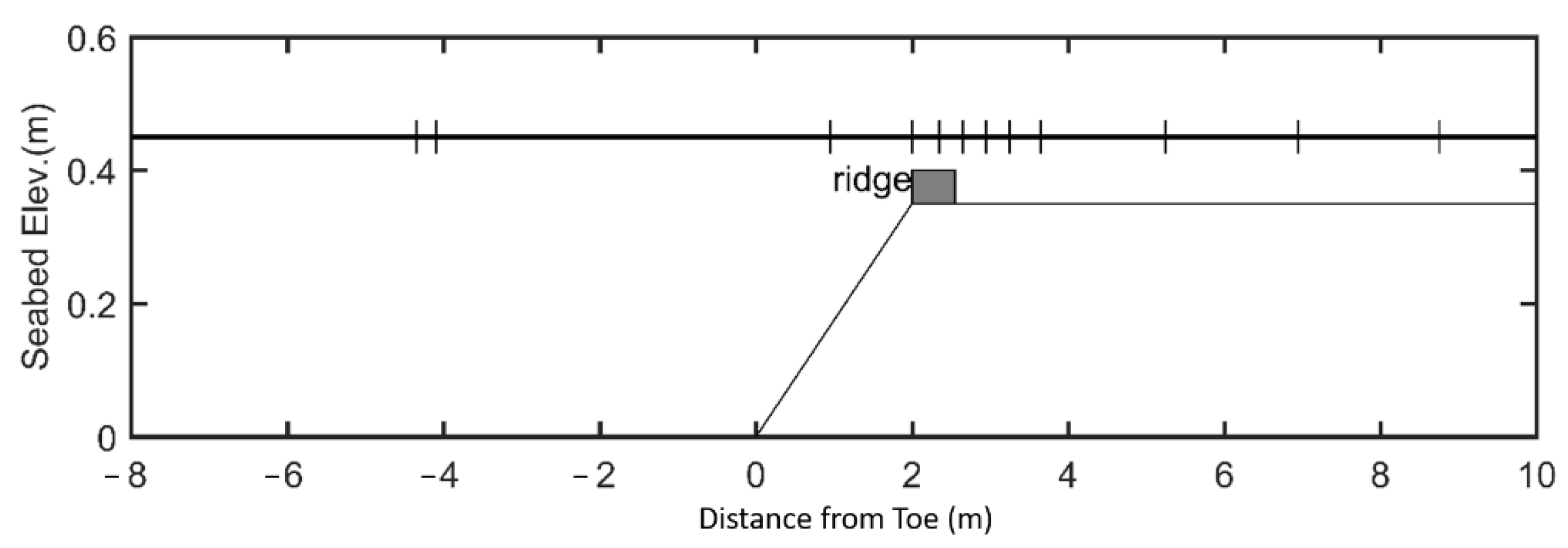
Yao et al. [1] conducted a list of experiments in wave propagation over fringing reefs in the Hydraulics Laboratory in Nanyang Technological University. Two representative cases for regular waves transformation on an idealized fringing reef with and without an idealized ridge are simulated in this study. The case without ridge is marked as Case 1, and the case where an idealized ridge is present is Case 2. Figure 1 shows the diagram of experimental terrain and the positions of the wave gauges. In the figure, the abscissa represents the distance from the toe of the reef, while the ordinate represents the seabed elevation. Twelve wave gauges were positioned. The reef slope was 1:6, the offshore water depth was 0.45 m, and the water depth over the reef top was 0.1 m. For Case 2, a rectangular box (55 cm long and 5 cm wide) was placed at the reef edge to mimic an idealized ridge. Sponge absorbing layers with a width of 5 m were installed at both sides of the domain. The incident wave height was 0.095 m and the wave period was 1.25 s.

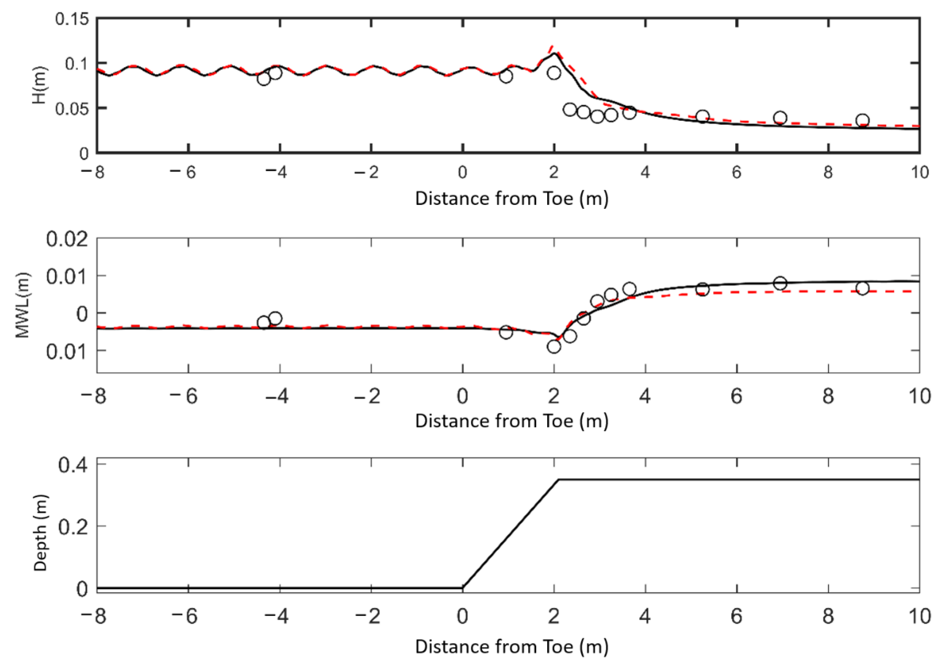
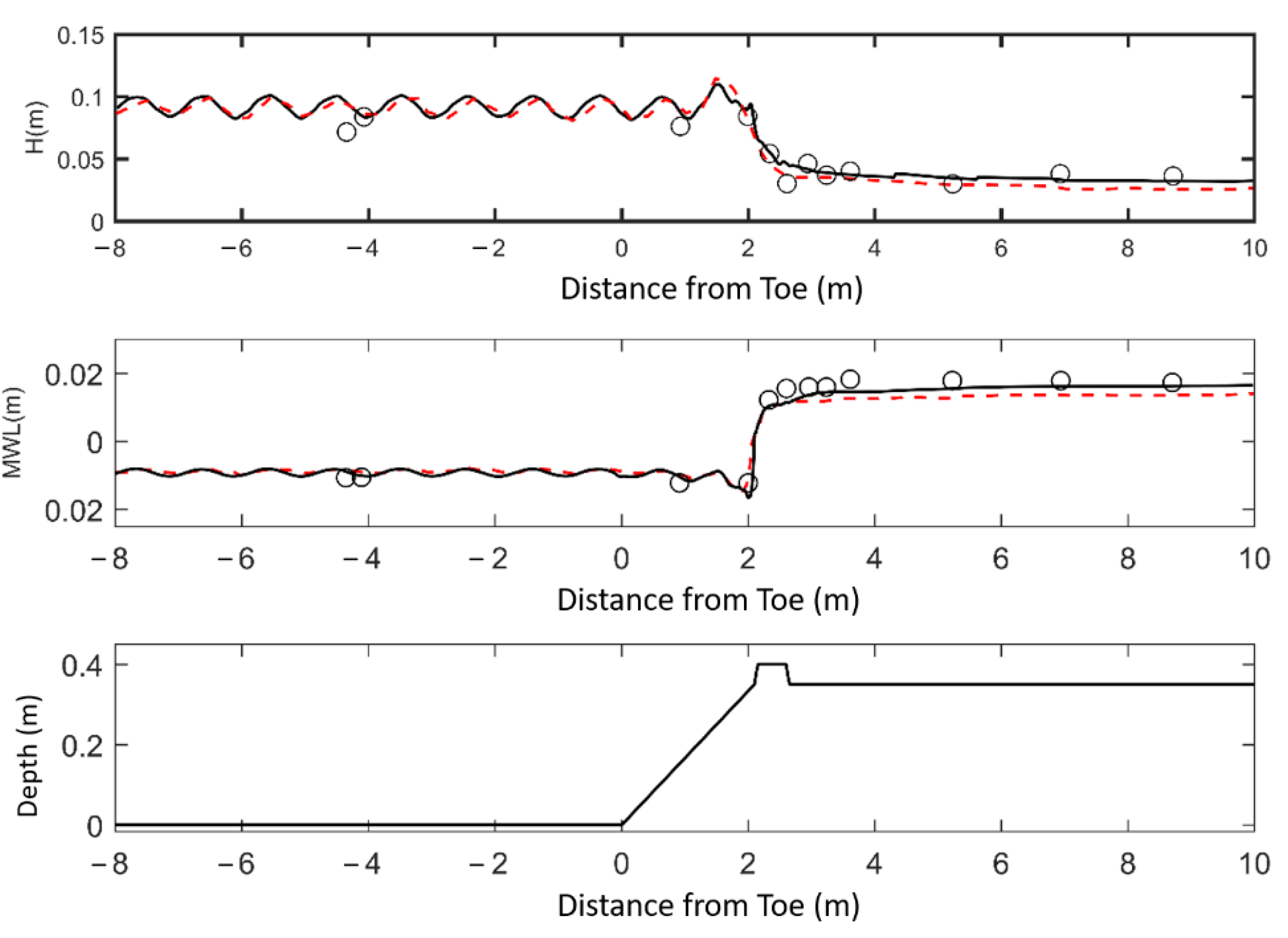
For monochromatic wave cases, the nested model is not adopted because computational time is relatively short. A grid size $dx=0.03\mathrm{m}$ and a time step $dt=0.01\mathrm{s}$ are used for simulation. The model is run for 100 wave periods and the last 40 wave periods are used for data analysis. Figure 2 and Figure 3 compare the simulated values with the measured values of wave height and mean water level of Case 1 and Case 2 respectively. Yao’s simulation result is also plotted in the figure to verify the simulation results of the present model.

Figure 2 and Figure 3 illustrate that before the reef slope, the predictions of the present model compare well with that of Yao, with the main differences concentrated in the swash zone and on the reef flat. The established model in this paper provides improved prediction of mean water level variation in both cases, especially for the wave setup on the reef flat. For Case 1 without a ridge, the wave setup is relatively small and has little effect on the wave height. For Case 2, the presence of the ridge leads to a notable increase of wave setup on the reef top, which in turn has a marked impact on the predicted wave height on the reef top. The improvement of the prediction of the wave setup by the present model results in an enhanced prediction of the wave height on the reef top.

4.2. Random Wave Transformation Over Steep Fringing Reefs

4.2.1. Model Setup

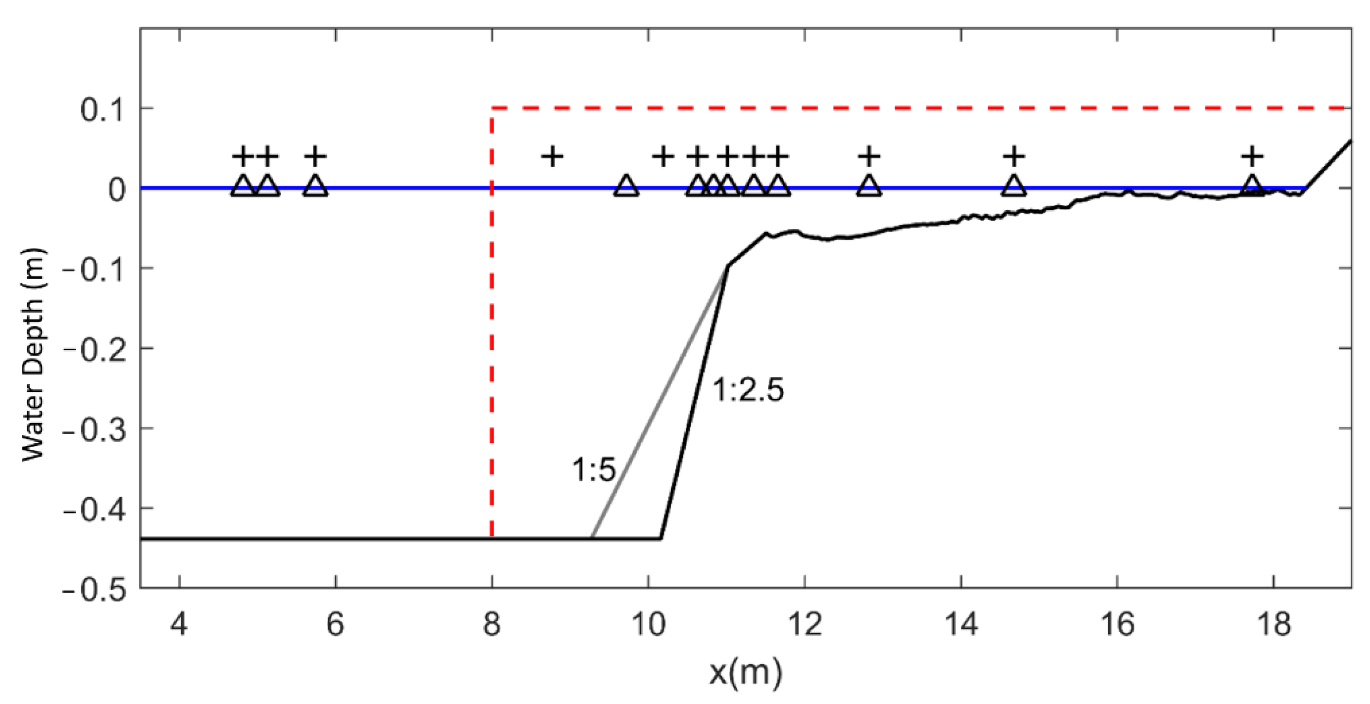
Based on actual bathymetry of Guam reefs, Smith et al. [45] simulated wave propagation, breaking, setup and runup on generalized reefs in a two-dimensional flume. The propagation experiment was conducted under three levels of tidal water, and two different slopes were selected. In the experiment, the surface of the reef was divided into smooth surface and rough surface. The acrylic reef surface was installed for the smooth-surface cases, and the reef surface applied paint mixed with roughening agent for the rough-surface cases. The reef flat is 7.3 m long with varying gentle slopes and the boundary at the far right is a 1:10 slope. Two reef slopes are 1:5 and 1:2.5. Figure 4 shows the diagram of experimental terrain and the positions of wave gauges. A total of 12 wave gauges are positioned and marked from left to right from WG1 to WG12. The positions of WG4 to WG6 are adjusted to different slopes as necessary. Randomized waves are made based on TMA spectrum for peak frequencies between 0.35 and 1.0 Hz.

Case 278 and Case 182 in Smith’s experiment are selected to conduct simulation in this study. These two cases correspond to 0.439 m off-reef water depth, with an incident significant wave height of 0.0792 m and peak period 0.99 s. Case 278 corresponds to a 1:5 reef slope with rough surface and Case 182 to a 1:2.5 reef slope with smooth surface. The computational setup is consistent with the experiment. A 5 m wide sponge absorbing layer is installed at the left end, internal wave maker is employed and Fourier analysis is conducted on the time series of the wave surface of WG1 to generate the corresponding internal wave signal for the desired wave. A one-way nesting model is employed in calculations. Less-refined grids and a second-order scheme are employed in the calculation of the whole computational domain, which is 20 m long and divided into 400 grids with the grid size of $dx=0.05\mathrm{m}$ and time step $dt=0.01\mathrm{s}$. Different coefficients of bottom friction are employed in the off-reef area ($f=0.002$) and reef flat ($f=0.2$).

4.2.2. Discussion of the Nested Model

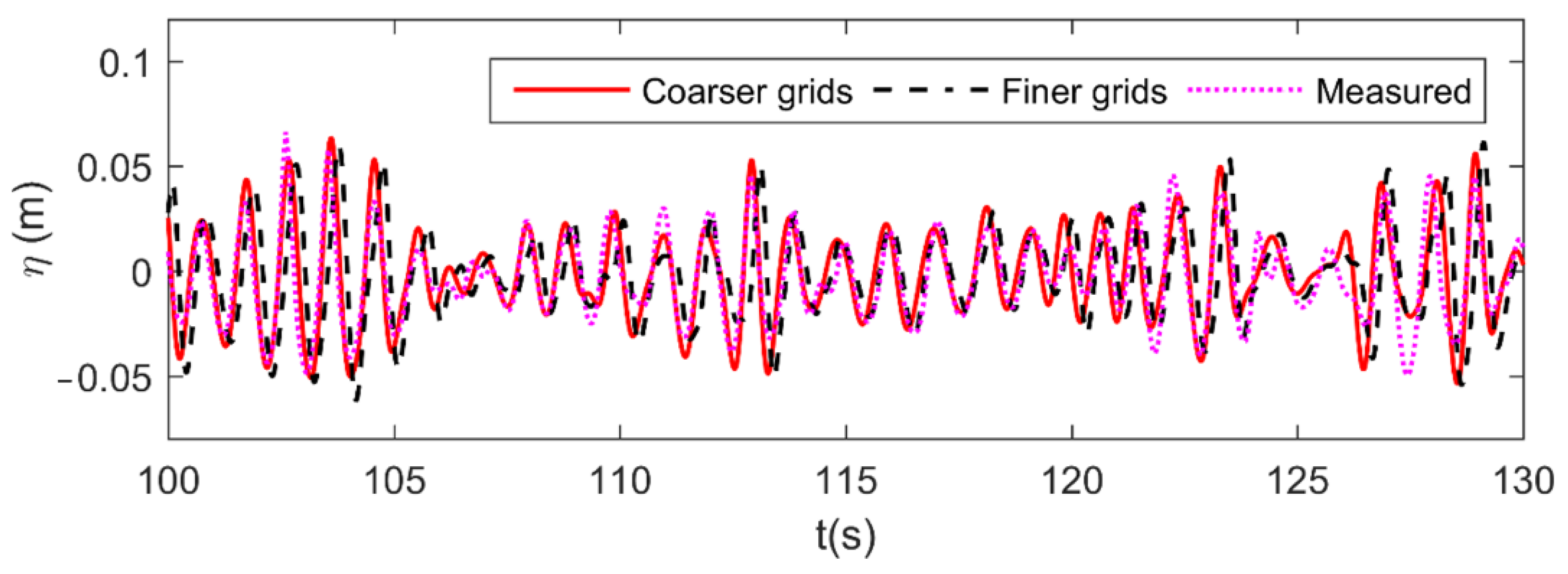
The nesting area with finer grids is located between 8 m to 20 m, as suggested by the red dashed line in Figure 4. Within the nested area, $dx=0.02\mathrm{m}$, $dt=0.005\mathrm{s}$ and the coefficient of friction remains the same. The nesting boundary must be located off the toe of the reef, where the bathymetry has not yet begun to change rapidly. In the first step of the one-way coupling, the calculation of the whole computational domain with coarser grids provides a time series of $u$ and $\eta$ at the nesting boundary for the next calculation step. In this step, the reflection and the return flow are taken into consideration and included in the time series of surface elevation and velocity at the nested boundary. The precision of the simulated reflection requires further testing, however. Figure 5 compares the simulated time series of Case 182 at WG4 by using different grid sizes, where WG4 is in the region of return flow. The size of coarser grids and that of finer grids are $dx=0.05\mathrm{m}$ and $dx=0.02\mathrm{m}$ individually. From the figure it can be seen that the simulation results of different grid sizes correspond well with each other and both give a satisfactory prediction of the measured value. This illustrates that the coarser grid adopted in the nested model is accurate enough for simulating reflection. A small phase difference exists because WG4 does not fall on the mesh points for coarser grids and the simulated value of the nearest grid point is adopted.

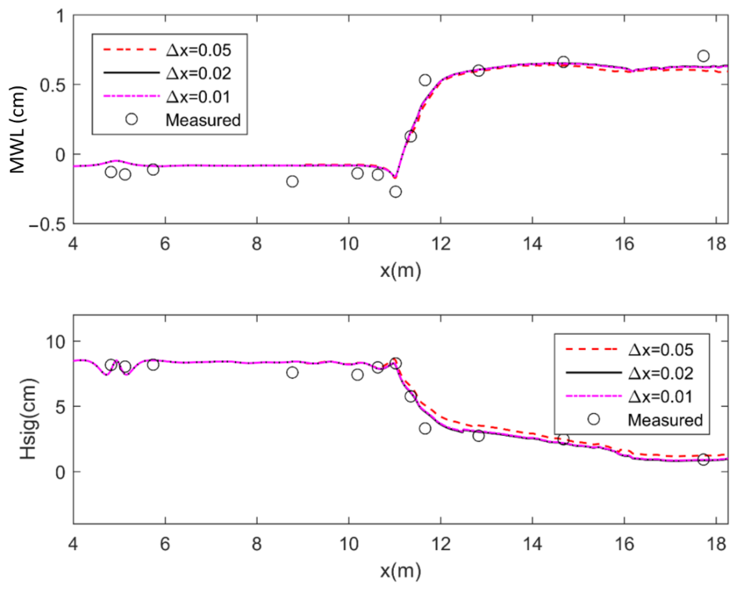
However, to better simulate the non-linear shoaling and capture of breaking point more accurately in the swash zone on a steep slope, finer grids are needed in the nested area. Determining optimum grid size is one of the key factors of the nested model and is very important for guaranteeing both the quality of the results and time-efficiency. The calculation of the coarser grid size in the first step of model coupling refers to the commonly used method of applying a Boussinesq-type model in slowly varying topography, where grid size approximately equals 1/60~1/40 of incident wavelength. The selected coarse grid size provides an accurate enough boundary condition for the nested area, as shown in Figure 5. To determine the grid size in the nested area, several simulations with different grid sizes are performed and the simulation results are compared in Figure 6.

From Figure 6 it can be seen that when grid size changes from $\Delta x=0.05\mathrm{m}$ to $\Delta x=0.02\mathrm{m}$, the simulated significant wave height improves remarkably, illustrating the necessity of the nested model. As the grid size becomes finer, the simulated result remains nearly unchanged. The value of the grid size in the nested area can be 1/3~1/2 of the coarse grid size, which is fine enough to gather accurate results in the swash zone.

Table 1. Comparison of central processing unit (CPU) time required for the fine-grid/non-nested and for the nested run.

Case No.	CPU Time (s)
	Fine Grid	Nested Model	Saved Time	Saving Ratio
278	5299.0	3033.0 (1896.5 + 1136.5) 1	2266.0	42.8%
182	5060.3	2949.7 (1842.6 + 1107.1)	2110.6	41.7%

¹ In the parentheses bold fonts is the CPU time of coarser grid in the whole computational domain.

compares the central processing unit (CPU) time of using fine grid in the whole domain (non-nested) and the time of the nested model. The CPU time of the nested model consists of two parts: The CPU time of applying coarser grids in the whole computational domain, and the CPU time of applying finer grids in the nested area. Use of the nested model enables one to save around 40% of the computational time which is needed when the finer mesh is applied to the whole domain.

4.2.3. Model Results and Discussion

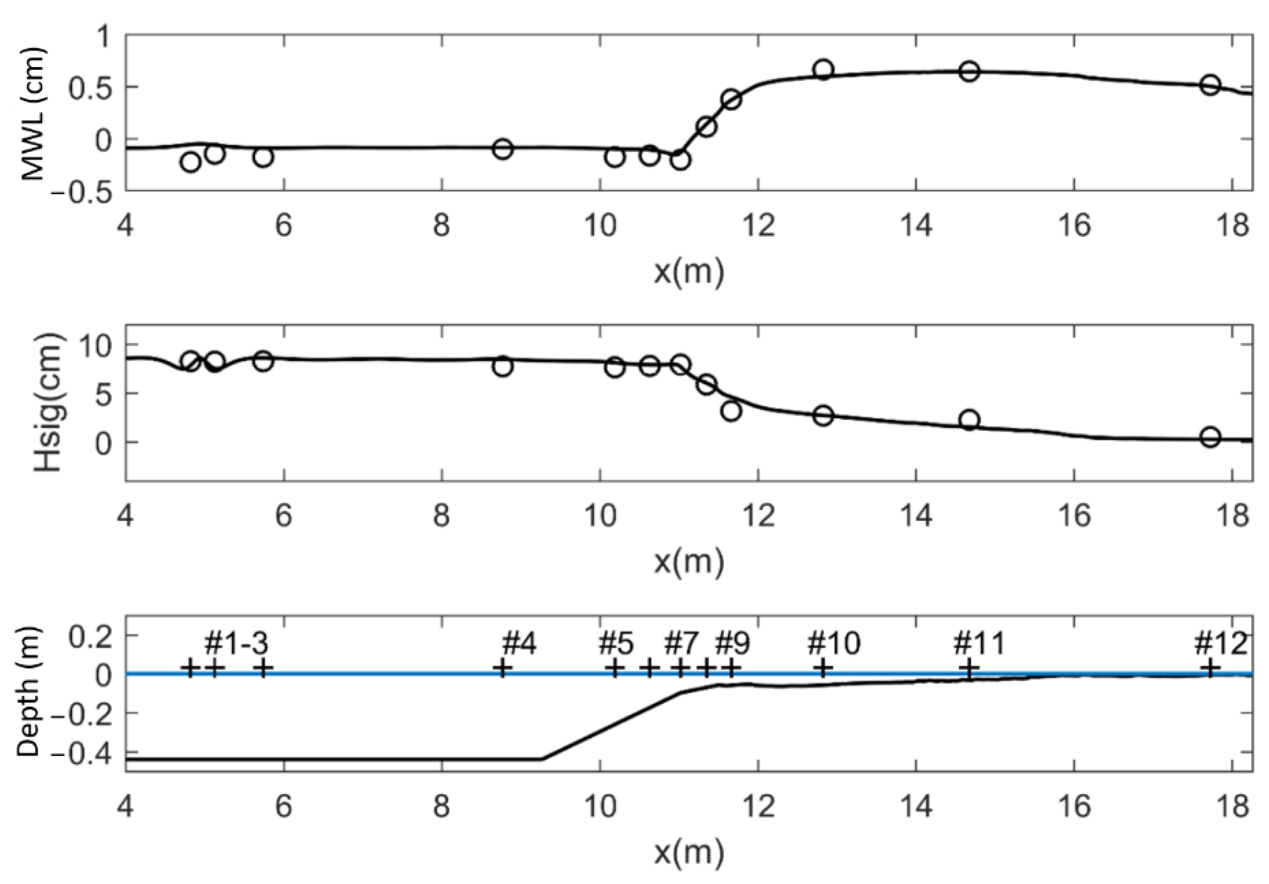
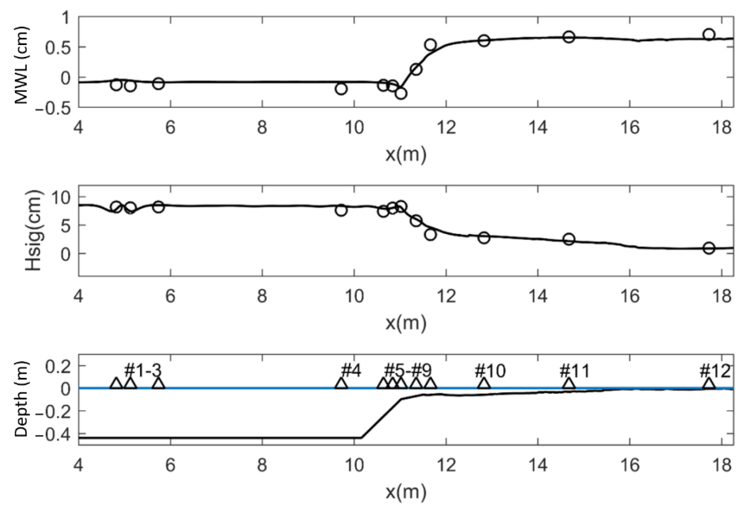
The present simulation lasted for 1200 s and the results of the last 720 s are used here for data analysis. Figure 7 and Figure 8 compares the simulated values with the measured values of significant wave height and mean water level of Case 278 and Case 182 respectively. The model accurately simulates the cross-reef variation of significant wave height, as well as wave setup on the reef flat, which are the most important criterion for assessing the applicability of the wave numerical model on reefs. To quantify performance of the numerical model assessed, the model skill [46] is introduced as:

$$\mathrm{skill}=1-\sqrt{\frac{\frac{1}{N}{\displaystyle \sum _{i=1}^N{(X_m^i-X_p^i)}^2}}{\frac{1}{N}{\displaystyle \sum _{i=1}^N{X_m^i}^2}}},$$

(35)

where $X_m$ represents measured value, $X_p$ calculated value, and $N$ is the position number of water gauge. For a nearly perfect model result, the value of skill would approach 1.

When it comes to actual construction, it is critical to accurately predict the wave setup on the reef flat, which is a key design factor. Table 1 lists the model skills of significant wave height (Hsig) and mean water level (MWL) under two cases as well as the model skills of the reef-flat wave setup (measured by WG7-WG12), and the ratios of the simulated value of maximum setup ${\eta }_p$ to the measured value ${\eta }_m$.

From

Table 2. Model skills and ratio of maximum wave setup of Case 278 and 182.

Case No.	Significant Wave Height (Hsig)	Mean Water Level MWL	Reef-Flat Wave Setup	${\mathit{\eta }}_{\mathit{p}}/{\mathit{\eta }}_{\mathit{m}}$
278	0.907	0.845	0.911	0.964
182	0.910	0.798	0.867	0.925

it can be seen that the model skills of significant wave height under both conditions are greater than 0.9, suggesting an accurate numerical simulation of wave height. Satisfactory accuracy is achieved in the simulation of wave setup on the steep reef slope and an even higher accuracy is achieved on a gentler slope. When the reef flat is the only concern, the model provides a superior degree of capability as it underestimates the maximum wave-induced setdown at breaking point which lowers the matching coefficient in the surf zone. The model can also predict the maximum wave setup with high accuracy.

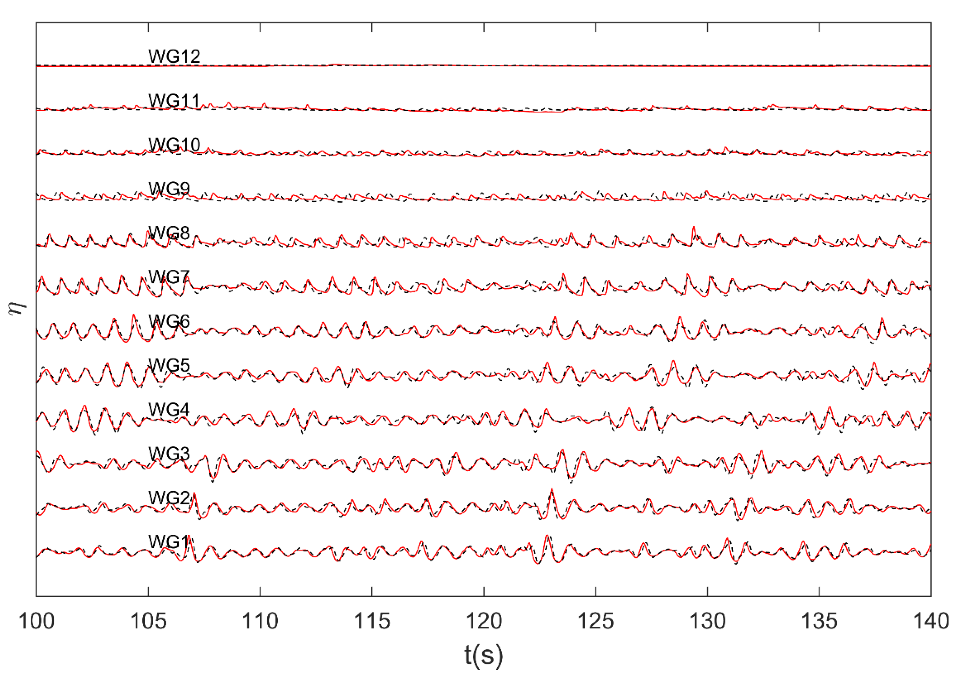
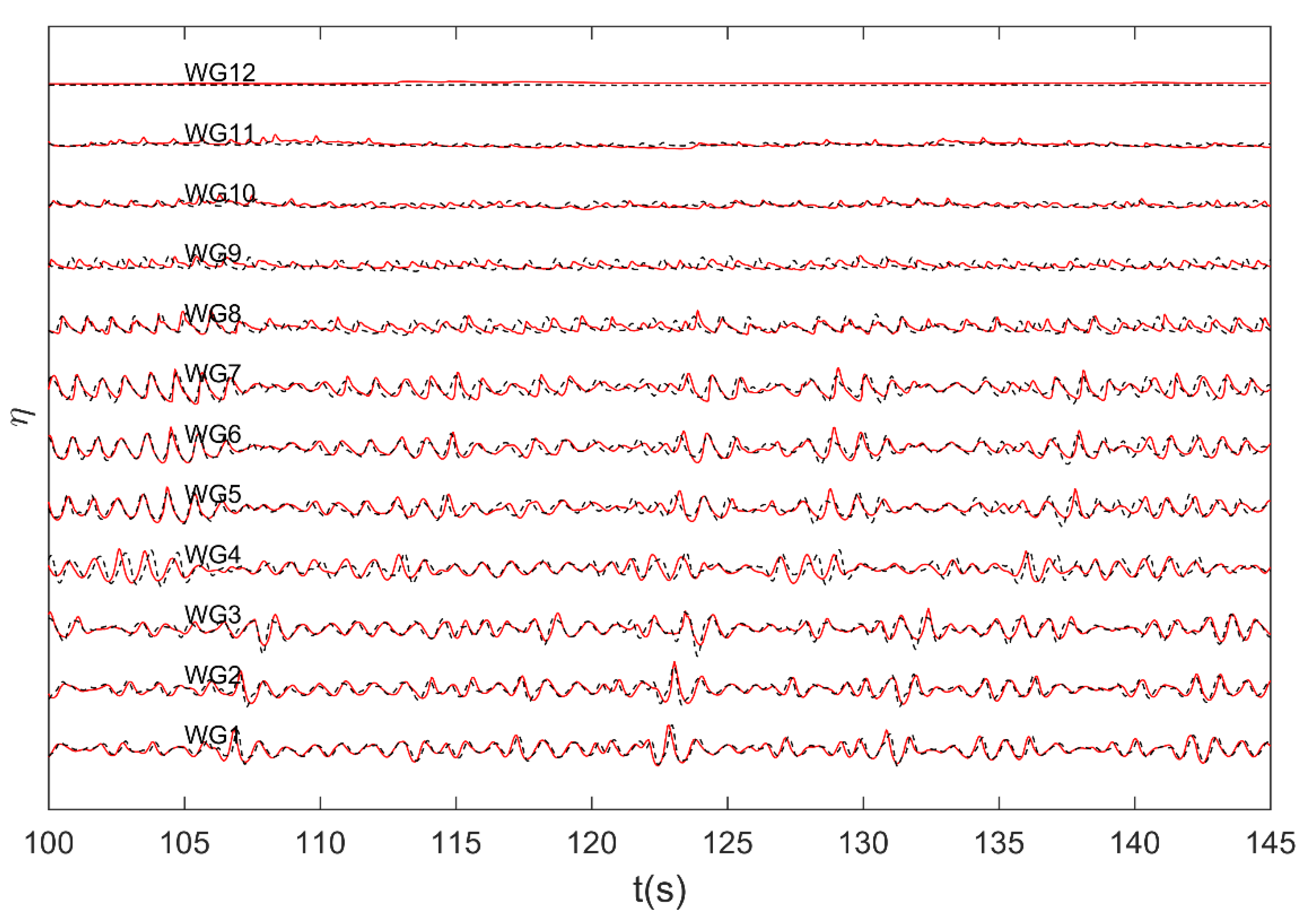
Figure 9 and Figure 10 compares time series of computed surface elevation from 100 s to 140 s with the measured data at all 12 gauges for case 278 and case 182. From bottom to top are the surface elevations at WG1 to WG12 and WG1 to WG3 show the results calculated with coarse meshing, while WG4 to WG12 illustrate the results calculated using the nested model with finer meshing. From the figure it can be seen that at WG1 to WG8, the time histories of experiment data and numerical result correspond well with each other, verifying the accuracy of the wave maker and nested model and illustrating that the numerical model can simulate non-linear wave shoaling well. At the positions of WG1 to WG12, the magnitude of calculated values and measured values is still in good agreement but displays a phase difference. This suggests that the model can provide an accurate simulation of energy dissipation but fails to reproduce the complex moving process of wave breaking with accuracy. This is because depth-integrated Boussinesq-type equations cannot describe the overturning of a free surface and the detailed breaking process, and the added empirical eddy viscosity model fails to reproduce all the details of wave breaking.

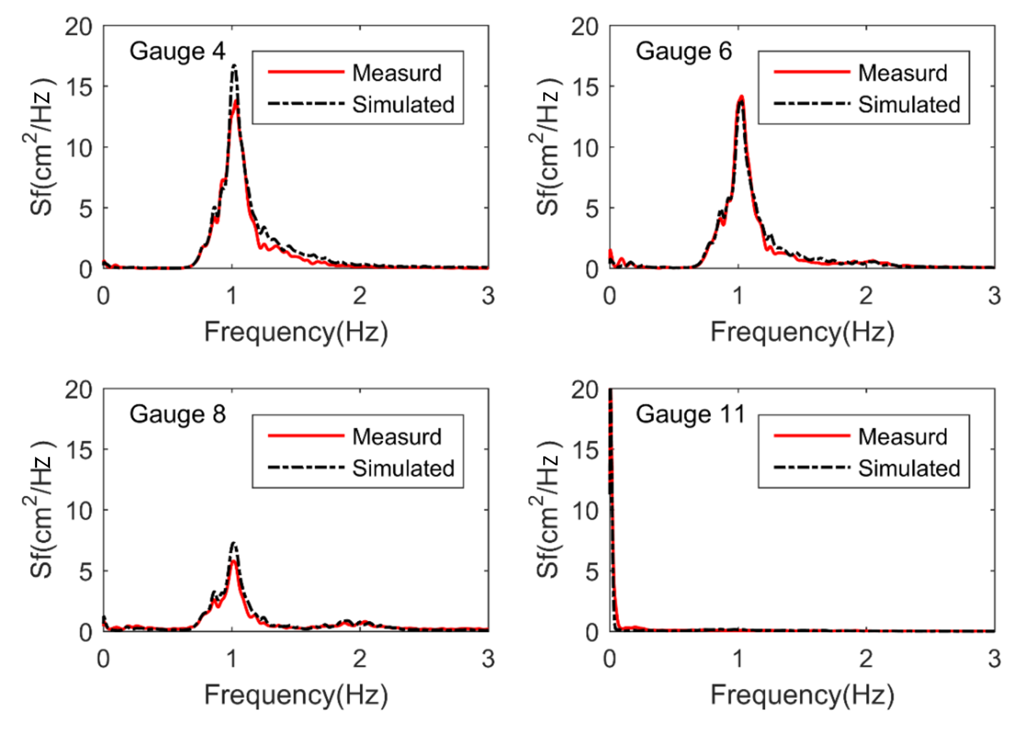
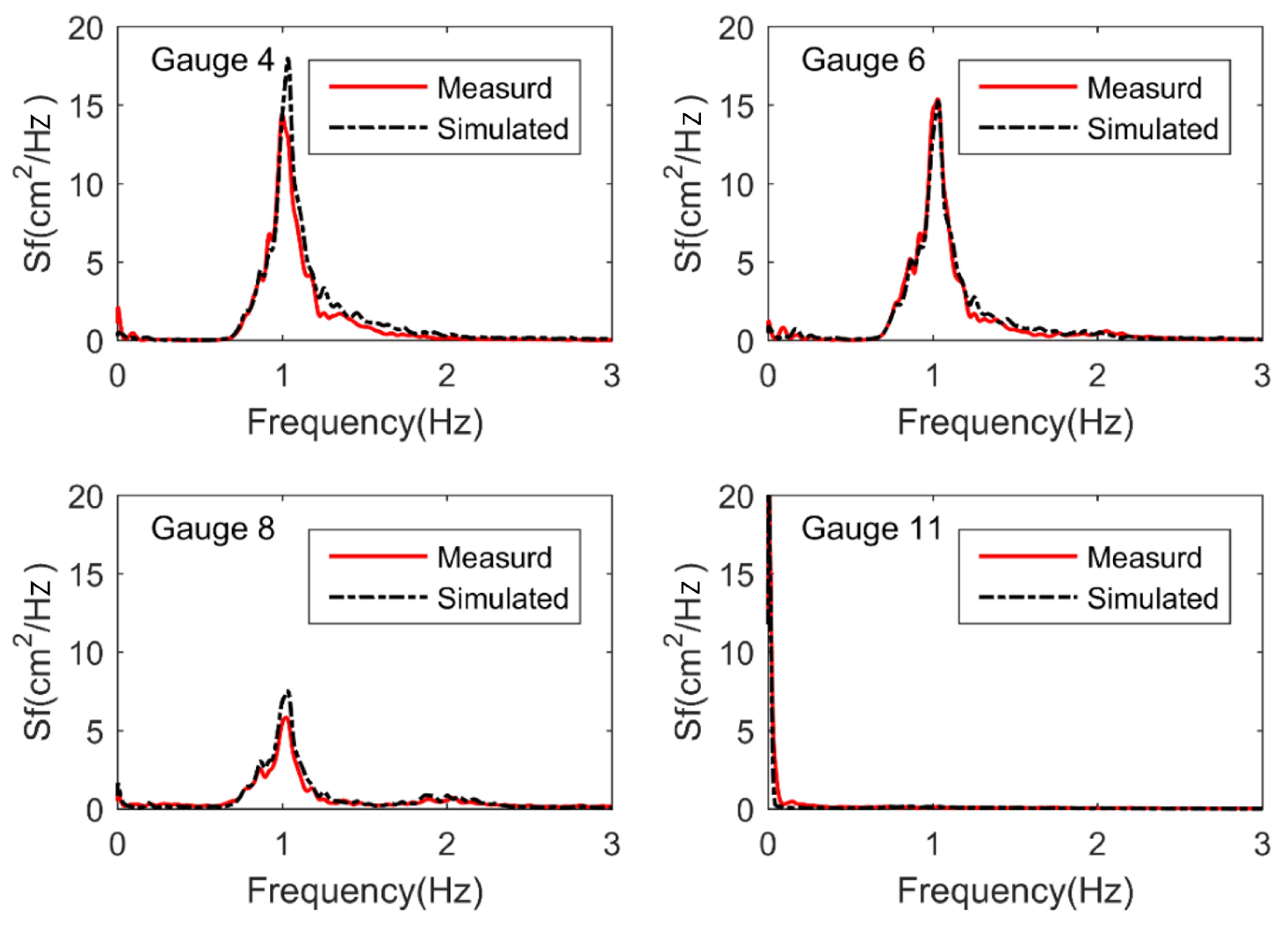
The breaking of random waves upon coral reef terrains is usually accompanied by energy transfer and results in a shift from high-frequency waves to low-frequency waves. Figure 11 and Figure 12 compare the measured and simulated wave energy spectra of four representative wave gauges for two cases. The four wave gauges selected are WG4 positioned off reef deep waters, WG6 on the reef slope, WG8 in the surf zone, and WG11 in the middle of the reef flat. From the figures it can be seen that as waves propagate from deep waters to reef flats, wave energy gradually transfers from spectral peak frequency to both higher and lower frequencies. High-order harmonics are generated at $f=2f_p$, and the manifestation of which is easily referred to wave energy spectra at WG6 and WG8. Waves break near the reef crest and a large part of the wave energy around the spectral peak frequency of incident waves is dissipated in the surf zone area, as shown by WG8. On the reef flat, the energy of incident waves continues to dissipate and when the waves reach WG11, positioned in the middle of the reef flat, wave energy is dominated by long gravity waves.

5. Conclusions

A numerical model is established in this study to simulate wave transformation, breaking, and setup on complex coral reef terrains with steep slopes. The model includes many modifications to better suit the topographic features of coral reefs. The main conclusions drawn are listed as follows:

• To better suit the steep terrain of coral reefs, the KLS09 Boussinesq-type equations is employed to establish a numerical wave model, as it is capable of describing rapidly varying bathymetry. A hybrid scheme of finite volume and finite difference is used to discretize equations to enhance stability and computational accuracy on complex terrains such as fringing reefs. When employing the finite volume method in the construction of interface flux, the Minmod–van-Leer mixed limiter is selected as most fitting for complex terrains.
• The nested model is established in accordance with the topographic characteristics of reefs as well as the requirements imposed by the hybrid limiter on meshing. In gentle slope areas, a finite volume method with coarse meshing and lower precision scheme is employed. In steep reef slope areas, as well as on reef flats, a finite volume method is employed with a far more refined meshing to improve both accuracy and time efficiency. This model can capture high-order harmonics with peak accuracy, also confirming the necessity of a nested model.
• An eddy viscosity method, modified to better suit steep terrains, is employed to simulate energy dissipation due to wave breaking. The breaker type is identified before the determination of wave-breaking parameters and piecewise uniform coefficients are used to process space-varying bottom friction.
• The verification of the model is conducted though laboratory experiments involving 1:5 and 1:2.5 reef slopes. Numerical results show that the employment of the nested model does not only save computing time but also retains high computational accuracy. The model can accurately simulate significant wave height and wave setup, especially on reef flats. As the reef slope increases, the simulation precision of mean water level slightly decreases, but remains a relatively high simulation accuracy of wave setup on the reef flat. In addition, the model can accurately simulate the energy transformation from a high-frequency to low-frequency wave during wave breaking with high accuracy. This result suggests the model is capable of predicting the generation of infragravity waves in the wave-breaking process. The numerical model established in this study can be applied in the design and construction of artificial islands to predict the change of wave height and wave setup on fringing reefs with steep slopes.

References

- Yao, Y.; Huang, Z.; Monismith, S.G.; Lo, E.Y.M. 1dh boussinesq modeling of wave transformation over fringing reefs. Ocean Eng. 2012, 47, 30–42. [Google Scholar] [CrossRef]
- Roeber, V.; Cheung, K.F. Boussinesq-type model for energetic breaking waves in fringing reef environments. Coast. Eng. 2012, 70, 1–20. [Google Scholar] [CrossRef]
- Metallinos, A.S.; Repousis, E.G.; Memos, C.D. Wave propagation over a submerged porous breakwater with steep slopes. Ocean Eng. 2016, 111, 424–438. [Google Scholar] [CrossRef]
- Gourlay, M. Wave set-up on coral reefs. 2. Set-up on reefs with various profiles. Coast. Eng. 1996, 28, 17–55. [Google Scholar] [CrossRef]
- FDINE. Code of Hydrology for Sea Harbour (jtj 213-98); FDINE: Tianjin, China, 1999. [Google Scholar]
- Kazolea, M.; Filippini, A.G.; Ricchiuto, M.; Abadie, S.; Medina, M.M.; Morichon, D.; Journeau, C.; Marcer, R.; Pons, K.; Le Roy, S. Wave Propagation Breaking, and Overtoping on a 2d Reef: A Comparative Evaluation of Numerical Codes for Tsunami Modelling; Research Report RR-9005; INRIA: Le Chesnay, France, 2016. [Google Scholar]
- Chella, M.A.; Bihs, H.; Myrhaug, D. Characteristics and profile asymmetry properties of waves breaking over an impermeable submerged reef. Coast. Eng. 2015, 100, 26–36. [Google Scholar] [CrossRef]
- Kamath, A.; Chella, M.A.; Bihs, H.; Arntsen, Ø.A. Energy transfer due to shoaling and decomposition of breaking and non-breaking waves over a submerged bar. Eng. Appl. Comput. Fluid Mech. 2017, 11, 450–466. [Google Scholar] [CrossRef]
- Tissier, M.; Bonneton, P.; Marche, F.; Chazel, F.; Lannes, D. A new approach to handle wave breaking in fully non-linear boussinesq models. Coast. Eng. 2012, 67, 54–66. [Google Scholar] [CrossRef]
- Tonelli, M.; Petti, M. Shock-capturing boussinesq model for irregular wave propagation. Coast. Eng. 2012, 61, 8–19. [Google Scholar] [CrossRef]
- Shi, F.; Kirby, J.T.; Harris, J.C.; Geiman, J.D.; Grilli, S.T. A high-order adaptive time-stepping tvd solver for boussinesq modeling of breaking waves and coastal inundation. Ocean Model. 2012, 43–44, 36–51. [Google Scholar] [CrossRef]
- Fang, K.; Zou, Z.; Dong, P.; Liu, Z.; Gui, Q.; Yin, J. An efficient shock capturing algorithm to the extended boussinesq wave equations. Appl. Ocean Res. 2013, 43, 11–20. [Google Scholar] [CrossRef]
- Roeber, V.; Cheung, K.F.; Kobayashi, M.H. Shock-capturing boussinesq-type model for nearshore wave processes. Coast. Eng. 2010, 57, 407–423. [Google Scholar] [CrossRef]
- Kirby, J.T. Boussinesq models and their application to coastal processes across a wide range of scales. J. Waterw. Port Coast. Ocean Eng. 2016, 142, 03116005. [Google Scholar] [CrossRef]
- Brocchini, M. A reasoned overview on boussinesq-type models: The interplay between physics, mathematics and numerics. Proc. Math. Phys. Eng. Sci. 2013, 469, 20130496. [Google Scholar] [CrossRef] [PubMed]
- Erduran, K.S.; Ilic, S.; Kutija, V. Hybrid finite-volume finite-difference scheme for the solution of boussinesq equations. Int. J. Numer. Methods Fluids 2010, 49, 1213–1232. [Google Scholar] [CrossRef]
- Nwogu, O.; Demirbilek, Z. Infragravity wave motions and runup over shallow fringing reefs. J. Waterw. Port Coast. Ocean Eng. 2010, 136, 295–305. [Google Scholar] [CrossRef]
- Su, S.-F.; Ma, G.; Hsu, T.-W. Boussinesq modeling of spatial variability of infragravity waves on fringing reefs. Ocean Eng. 2015, 101, 78–92. [Google Scholar] [CrossRef]
- Fang, K.-Z.; Yin, J.-W.; Liu, Z.-B.; Sun, J.-W.; Zou, Z.-L. Revisiting study on boussinesq modeling of wave transformation over various reef profiles. Water Sci. Eng. 2014, 7, 306–318. [Google Scholar]
- Ding, J.; Tian, C.; Wang, Z.; Ling, H.; Li, Z. Experimental research on wave deformation near the typical island. Chin. J. Hydrodyn. 2015, 30, 194–200. [Google Scholar]
- Kim, G.; Lee, C.; Suh, K.-D. Extended boussinesq equations for rapidly varying topography. Ocean Eng. 2009, 36, 842–851. [Google Scholar] [CrossRef]
- Madsen, P.A.; Sørensen, O.R. A new form of the boussinesq equations with improved linear dispersion characteristics. Part 2. A slowly-varying bathymetry. Coast. Eng. 1992, 18, 183–204. [Google Scholar] [CrossRef]
- Nwogu, O. Alternative form of boussinesq equations for nearshore wave propagation. J. Waterw. Port Coast. Ocean Eng. 1993, 119, 618–638. [Google Scholar] [CrossRef]
- Madsen, P.A.; Fuhrman, D.R.; Wang, B. A boussinesq-type method for fully nonlinear waves interacting with a rapidly varying bathymetry. Coast. Eng. 2006, 53, 487–504. [Google Scholar] [CrossRef]
- Booij, N. A note on the accuracy of the mild-slope equation. Coast. Eng. 1983, 7, 191–203. [Google Scholar] [CrossRef]
- Li, Y.-S.; Zhan, J.-M.; Su, W. Chebyshev finite spectral method for 2-d extended boussinesq equations. J. Hydrodyn. Ser. B 2011, 23, 1–11. [Google Scholar] [CrossRef]
- Kazolea, M.; Delis, A.I. A Well-Balanced Shock-Capturing Hybrid Finite Volume-Finite Difference Numerical Scheme for Extended 1d Boussinesq Models; Elsevier Science Publishers B. V.: London, UK, 2013; pp. 167–186. [Google Scholar]
- Darvishi, E.; Fenton, J.D.; Kouchakzadeh, S. Boussinesq equations for flows over steep slopes and structures. J. Hydraul. Res. 2016, 55, 324–337. [Google Scholar] [CrossRef]
- Calabrese, M.; Buccino, M.; Pasanisi, F. Wave breaking macrofeatures on a submerged rubble mound breakwater. J. Hydro-Environ. Res. 2008, 1, 216–225. [Google Scholar] [CrossRef]
- Zhou, J.G.; Causon, D.M.; Mingham, C.G.; Ingram, D.M. The surface gradient method for the treatment of source terms in the shallow-water equations. J. Comput. Phys. 2001, 168, 1–25. [Google Scholar] [CrossRef]
- Choi, Y.-K.; Seo, S.-N. Wave transformation using modified funwave-tvd numerical model. J. Korean Soc. Coast. Ocean Eng. 2015, 27, 406–418. [Google Scholar] [CrossRef]
- Kennedy, B.; Chen, Q.; Kirby, J.T.; Dalrymple, R.A. Boussinesq modeling of wave transformation, breaking, and runup i: 1d. J. Waterw. Port Coast. Ocean Eng. 2000, 126, 39–47. [Google Scholar] [CrossRef]
- Schäffer, H.A.; Madsen, P.A.; Deigaard, R. A boussinesq model for waves breaking in shallow water. Coast. Eng. 1993, 20, 185–202. [Google Scholar] [CrossRef]
- Bruno, D.; De Serio, F.; Mossa, M. The FUNWAVE model application and its validation using laboratory data. Coastal Eng. 2009, 56, 773–787. [Google Scholar] [CrossRef]
- Tonelli, M.; Petti, M. Hybrid finite volume—Finite difference scheme for 2dh improved boussinesq equations. Coast. Eng. 2009, 56, 609–620. [Google Scholar] [CrossRef]
- Kazolea, M.; Ricchiuto, M. On wave breaking for boussinesq-type models. Ocean Model. 2018, 123, 16–39. [Google Scholar] [CrossRef]
- Chen, Q.; Kirby, J.T.; Dalrymple, R.A.; Kennedy, A.B.; Chawla, A. Boussinesq modeling of wave transformation, breaking, and runup. Ii: 2d. J. Waterw. Port Coast. Ocean Eng. 2000, 126, 48–56. [Google Scholar] [CrossRef]
- Chondros, M.K.; Koutsourelakis, I.G.; Memos, C.D. A boussinesq-type model incorporating random wave-breaking. J. Hydraul. Res. 2011, 49, 529–538. [Google Scholar] [CrossRef]
- Kirby, J.T.; Wei, G.; Chen, Q.; Kennedy, A.B.; Dalrymple, R.A. Funwave 1.0. Fully Nonlinear Boussinesq Wave Model. Documentation and User’s Manual; University of Delaware: Newark, DE, USA, 1998. [Google Scholar]
- Israeli, M.; Orszag, S.A. Approximation of radiation boundary conditions. J. Comput. Phys. 1981, 41, 115–135. [Google Scholar] [CrossRef]
- Wei, G.; Kirby, J.T.; Sinha, A. Generation of waves in boussinesq models using a source function method. Coast. Eng. 1999, 36, 271–299. [Google Scholar] [CrossRef]
- Francesca, D.S.; Michele, M. Experimental study on the hydrodynamics of regular breaking waves. Coastal Eng. 2006, 53, 99–113. [Google Scholar] [CrossRef]
- De Serio, F.; Mossa, M. Numerical simulation of infragravity waves in fringing reefs using a shock-capturing non-hydrostatic model. Ocean Eng. 2014, 85, 54–64. [Google Scholar] [CrossRef]
- De Serio, F.; Mossa, M. A laboratory study of irregular shoaling waves. Exp. Fluids 2013, 54, 1536. [Google Scholar] [CrossRef]
- Smith, E.R.; Hesser, T.J.; Smith, M.K. Two- and Three-Dimensional Laboratory Studies of Wave Breaking, Dissipation, Setup, and Runup on Reefs. ERDC/CHLTR-12-21; U.S. Army Engineer Research and Development Center: Vicksburg, MS, USA, 2012. [Google Scholar]
- Gallagher, E.L.; Steve, E.; Guza, R.T. Observations of sand bar evolution on a natural beach. J. Geophys. Res. Oceans 1998, 103, 3203–3215. [Google Scholar] [CrossRef] [Green Version]
Figure 1.
Cross shore profiles of reef bathymetry and wave gauge locations in Yao’s experiment.
Figure 2.
Variation of wave height and mean water level over the reef profile for Case 1. Black solid line: predictions by present model; red dashed line: predictions by Yao; open circles: laboratory measurements.
Figure 3.
Variation of wave height and mean water level over the reef profile for Case 2. Black solid line: predictions by present model; red dashed line: predictions by Yao; open circles: laboratory measurements.
Figure 4.
Cross shore profiles of reef bathymetry and wave gauge locations. The grey line represents a 1:5 slope and black line 1:2.5. The positions of wave gauge are marked by “Δ” for the 1:2.5 slope experiment, and “+” for the 1:5 slope experiment. The red dashed frame is the nesting area.
Figure 5.
Comparison of the time series of wave surfaces at WG4 with different grid sizes. Red solid line: predictions with grid size dx = 0.05 m; black dashed line: predictions with grid size dx = 0.02 m; pink dotted line: laboratory measurements.
Figure 6.
Comparison of simulation results with different nested grid sizes.
Figure 7.
Variation of the significant wave height and mean water level over the reef profile for Case 278. Solid line: predictions by present model; open circles: laboratory measurements.
Figure 8.
Variation of the significant wave height and mean water level over the reef profile for Case 182. Solid line: predictions by present model; open circles: laboratory measurements.
Figure 9.
Comparison of the time series of wave surfaces for case 278. Red lines in the figure are measured data and black dashed lines are simulated results.
Figure 10.
Comparison of the time series of wave surfaces for case 182. Red lines in the figure are measured data and black dashed lines are simulated results.
Figure 11.
Comparison between the computed and measured wave energy spectra of four representative wave gauges for Case 278.
Figure 12.
Comparison between the computed and measured wave energy spectra of four representative wave gauges for Case 182.