Application of the 2D Depth-Averaged Model, FLATModel, to Pumiceous Debris Flows in the Amalfi Coast

1
Department of Civil Engineering, University of Salerno, Via Giovanni Paolo II, 132, 84084 Fisciano SA, Italy
2
CIMNE—International Centre for Numerical Methods in Engineering, Universitat Politècnica de Catalunya, C/Gran Capità S/N, 08034 Barcelona, Spain
*
Authors to whom correspondence should be addressed.
Water 2018, 10(9), 1159; https://doi.org/10.3390/w10091159
Submission received: 31 July 2018
/
Revised: 14 August 2018
/
Accepted: 20 August 2018
/
Published: 29 August 2018
(This article belongs to the Special Issue Landslide Hydrology)
Abstract
:Few studies about modelling pumice debris flows are available in literature. An integrated approach based on field surveys and numerical modelling is here proposed. A pumiceous debris flow, which occurred in the Amalfi Coast (Italy), is reconstructed by the numerical code, FLATModel, consisting of a two-dimensional shallow-water model written in curvilinear coordinates. The morphological evolution of the gully and of the alluvial fan was monitored by terrestrial laser scanner and photo-modelling aerial surveys, providing, in a cost-effective way, data otherwise unavailable, for the implementation, calibration and validation of the model. The most suitable resistance law is identified to be the Voellmy model, which is found capable of correctly describing the friction-collisional resistance mechanisms of pumiceous debris flows. The initial conditions of the numerical simulations are assumed to be of dam-break type: i.e., they are given by the sudden release of masses of pumice, whose shape and depths are obtained by reconstruction of the pre-event slopes. The predicted depths and shape of deposits are compared with the measured ones, where a good agreement (average error smaller than 10 cm) is observed for several dam-break scenarios. The proposed cost-effective integrated approach can be straightforwardly employed for the description of other debris flows of the same kind and for better designing risk mitigation measures.
1. Introduction
In mountainous areas, debris flows and rock/snow avalanches represent an important hazard for mankind and infrastructures [1,2,3]. In the last decades, these phenomena have attracted huge interest from the scientific community, due to the increasing need to correctly describe their initiation and propagation phases, in order to better assess the risk, demarcate the hazardous areas and develop risk mitigation measures. Besides the theoretical and laboratory experimental investigations on the dynamics of granular flows and granular-liquid mixtures [4,5,6,7,8,9,10], considerable efforts have been recently made in the description of these flows at the field scale [11,12,13,14,15,16]. Modelling the propagation stages of these flows involves mathematical complexity and advanced numerical simulation techniques [17,18,19,20,21,22]. Dealing with convective terms requires specific solvers and algorithms. In the case of debris flows (DF), different from clear water flows, there are extra elements that challenge the model development. The main specific issues to be addressed are the scale of the problem and the rheology of the mixture. A debris flow is a natural hazard with a characteristic scale of order of hundreds/thousand metres, meaning that the computational domain is large and, hence, the choice of the mesh size is crucial. From a practical viewpoint this typically involves vertical integration and averaging of the hydraulic variables, leading to models of the shallow-water type [23,24,25,26].
Moreover, the evaluation of the energy losses during the flow has to be suitably addressed. Generally speaking, a debris flow is made up of a heterogeneous mixture of solids and liquids. In nature, the fluid is water or a slurry of water and fine sediments (clay and silt), and the solid phase is represented by natural grain soils, with a size ranging from silt to boulders. The physics governing the mixture behaviour at the micro-scale is fully defined by the classical equations of mechanics, taking into account interactions within the solid phase, solid-fluid interactions and the dynamics of the fluid phase. Yet, modelling one by one every single particle in problems at the field scale becomes highly computationally expensive, and, often, is still beyond the capacities of the existing computational resources. Therefore, a macro-scale rheological approach should be selected, moving from the particle-fluid mechanics to the continuum mechanics. The scientific problem of the debris flow rheology is a consequence of this continuum mechanics approach, e.g., [27,28].
The code FLATModel, firstly introduced by [20] and subsequently reformulated in curvilinear coordinates in [29], implements a two-dimensional depth-averaged mathematical model of the shallow-water type, specifically designed to describe the propagation of debris flows over irregular mountainous topographies. The model, which can be equipped with different basal resistance laws from various rheological assumptions, is numerically integrated through an explicit finite volume shock-capturing scheme. FLATModel is, here, employed to reconstruct a pumice DF, which occurred in the Amalfi Coast (Province of Salerno, Italy) in October 2013. The digital terrain model (DTM) of the debris fan, before and after the event, was surveyed by terrestrial laser scanner (TLS). Moreover, the entire topography up to the debris flow scars (i.e., the initiation zones) was obtained by photo-modeling analysis of digital pictures, taken by an aerial survey carried out through a drone, i.e., an unmanned aerial vehicle (UAV) [30]. Different possible dam-break scenarios are investigated for the numerical reconstruction of the DF event. From this investigation it emerges that the shape of deposit can be properly described by employing a Voellmy-type resistance law [31,32], which only requires the calibration of two parameters. It suggests that the Voellmy resistance law is capable of describing the essential momentum exchange mechanisms, of frictional and collisional type, occurring in pumice granular flows. Moreover, it is noteworthy to anticipate that the best agreement with the survey data is found in the scenario, where two subsequent dam-break waves take place in rapid succession. In fact, in this scenario the numerical simulation better captures the flow dynamics, especially during the final deposition stages of the granular material on the alluvial fan.
The paper is composed of the following parts. Section 2 is devoted to a brief description of the mathematical model, the related numerical implementation (Section 2.1), and the site under study and the field surveys (Section 2.2). The numerical reconstruction of the pumice DF is reported in Section 3 and is discussed in Section 4. The conclusions are summarized in Section 5.
2. Materials and Methods
2.1. The Mathematical Model
Within the framework of continuum mechanics and under the assumption that the characteristic flow length is much larger than the flow depth, a popular and cost-effective mathematical approach for describing the propagation of geophysical flows and floods is represented by shallow-water type models, e.g., [17,18,19,20,24,25]. Renouncing to the complete description of the velocity field along the flow depth, e.g., [17], such kind of models are parsimonious of parameters and require much lower computational efforts compared to fully three-dimensional models. In field-scale investigations, it is customary to calibrate the model parameters through back-analysis of field data [11,19,20]. The original code FLATModel, here employed, belongs to this family of models and is specifically designed to describe the DFs propagation on irregular topographies.
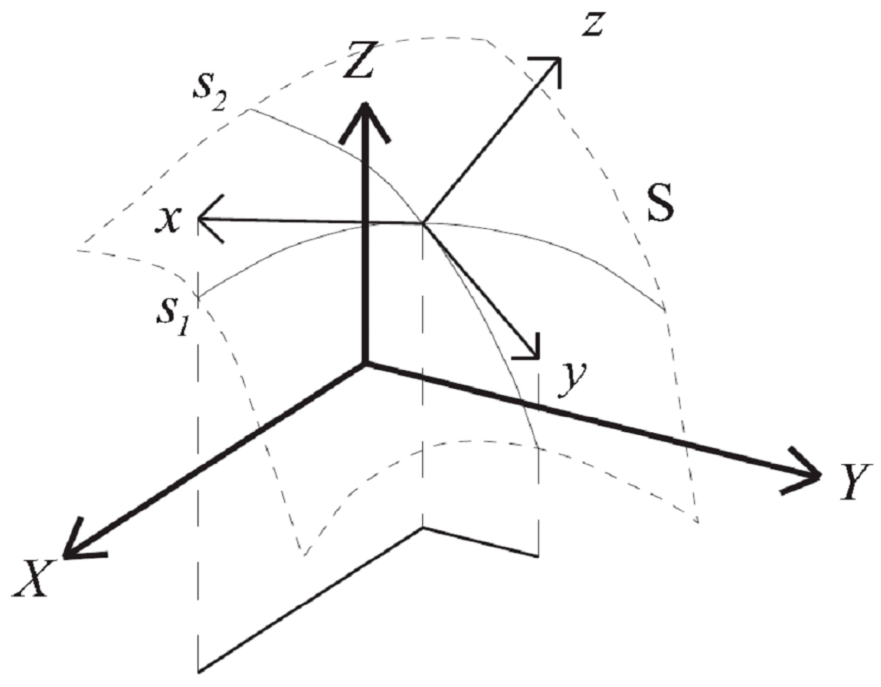
There is a fundamental relation between the selected coordinate system, the equation system and the discretization used in the solver [24,25,33,34]. The coordinate system proposed in FLATModel [29] is shown in Figure 1, where the local coordinates are labelled x, y.
The obtained equation system is devoted to steep slopes, while it neglects the curvature effects. No particular analysis on the effects of the curvature was performed; thus, validation cases are used as the methodology to justify the model performance. However, some preliminary curvature tensor analyses, reported in [29], indicate that curvature effects could be important solely near the fan apex, where the slope changes suddenly. The mass and momentum balance equations of the model, which are obtained by depth-integration of the local balance equations along the flow depth and subsequent shallow-water approximation, are
where h is depth, t is time, g is the metric tensor, uk is the k-th component of the velocity vector, gi is the gravity vector, xk is the k-th space coordinate, Tij is the stress tensor, ρ is the density and τbi the bed shear stress, to be defined by a specific rheology. As the proposed coordinate system is not orthogonal, the cross terms appear in the Equations. For more details about the model, we refer the Reader to [20,29].
To assess the term τbi in (1), FLATModel is capable of employing the most popular basal resistance laws for mud flows and debris flows (e.g., Herschel-Bulkley, Bingham, Coulomb frictional and Voellmy resistance laws). The partial differential Equation system (1), is numerically integrated by using an explicit shock-capturing finite-volume scheme, based on the Harten-Lax-Leer-Contact (HLLC) approximate Riemann solver [35]. All the numerical simulations, hereafter reported, were performed by using the pre-event DTM as basal topography on the alluvial fan and the DTM, obtained by aerial survey, as basal topography in the rest of the spatial domain. The topography, obtained from merging the two DTMs, was suitably downscaled for all the numerical simulations, employing a mesh of size 0.1 m.
2.2. Study Area
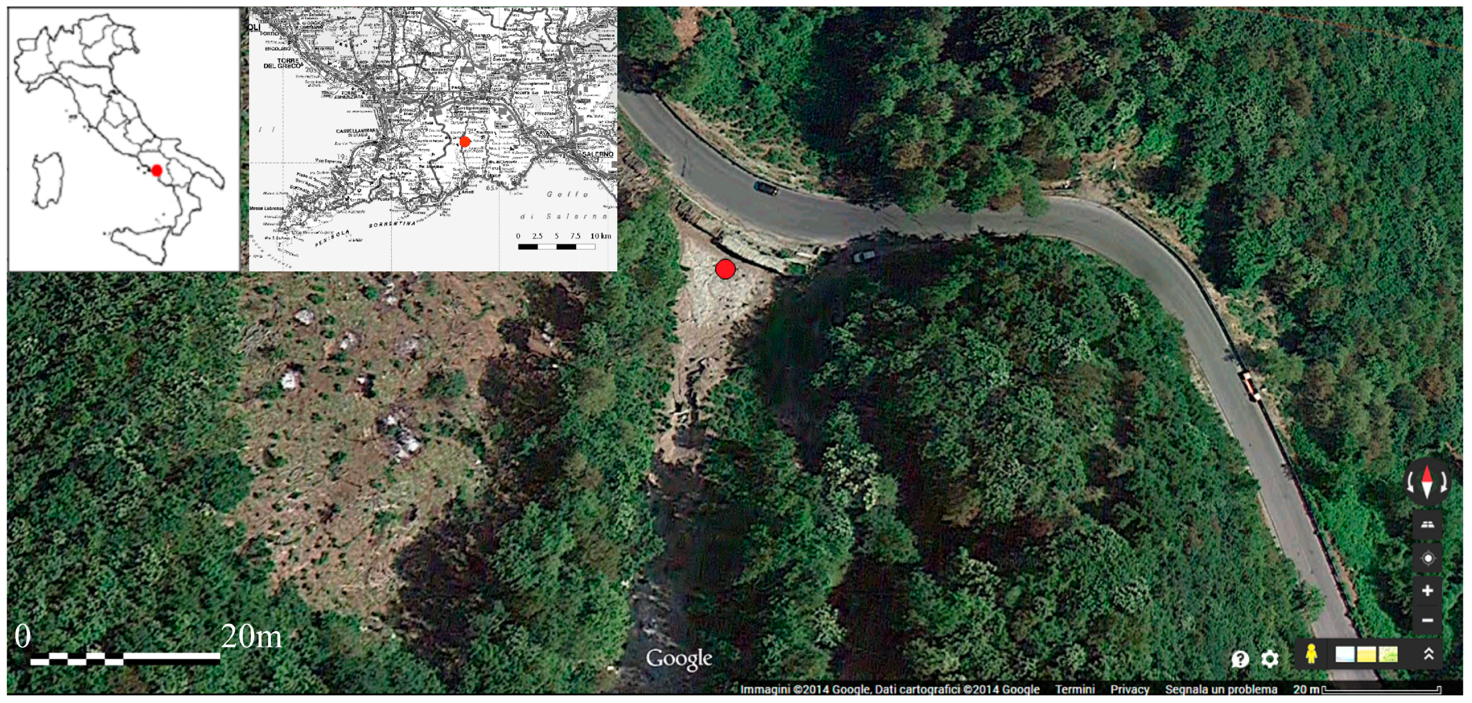
The site under study is a gully located in a small basin of Lattari Mountains, belonging to the municipality of Tramonti in the Amalfi Coast (Campania region, Italy) and often concerned by pumiceous debris flows. The overall extension of the basin is about 5 ha and its average altitude is 780 m a.s.l. The gully intersects the Provincial road, SP1, connecting the towns of Ravello and Tramonti, at coordinates 40.690910° N–14.613087° E, as it is shown by the satellite view reported in Figure 2. It is worth noting that other three active gullies, as well concerned by pumiceous DF events, intersect the same road along a tract approximately 400 m-long and, thus, contribute to further increase the DF hazard on the road infrastructure. The pyroclastic soils covering the carbonatic rock of the Campanian Appennine are well-known to be affected by DF events [28,36,37,38]. Such deposits date back to the various volcanic eruptions of the Somma-Vesuvius volcano, which is located ≈20 km North-West of the Lattari Mountains. The soil stratigraphy of the area is mainly composed of limestone bedrock, covered by pumice and ash layers, which are intercalated by paleo-soils of fine sediments [39,40]. In particular, pumice lenses, with thickness up to a few meters are often present, and are mainly dated back to the Plinian volcanic eruption of 79 A.D., during which the prevailing wind direction was South-East and, thus, a conspicuous amount of lightweight pyroclastic sediments deposited on the Lattari Mountains.
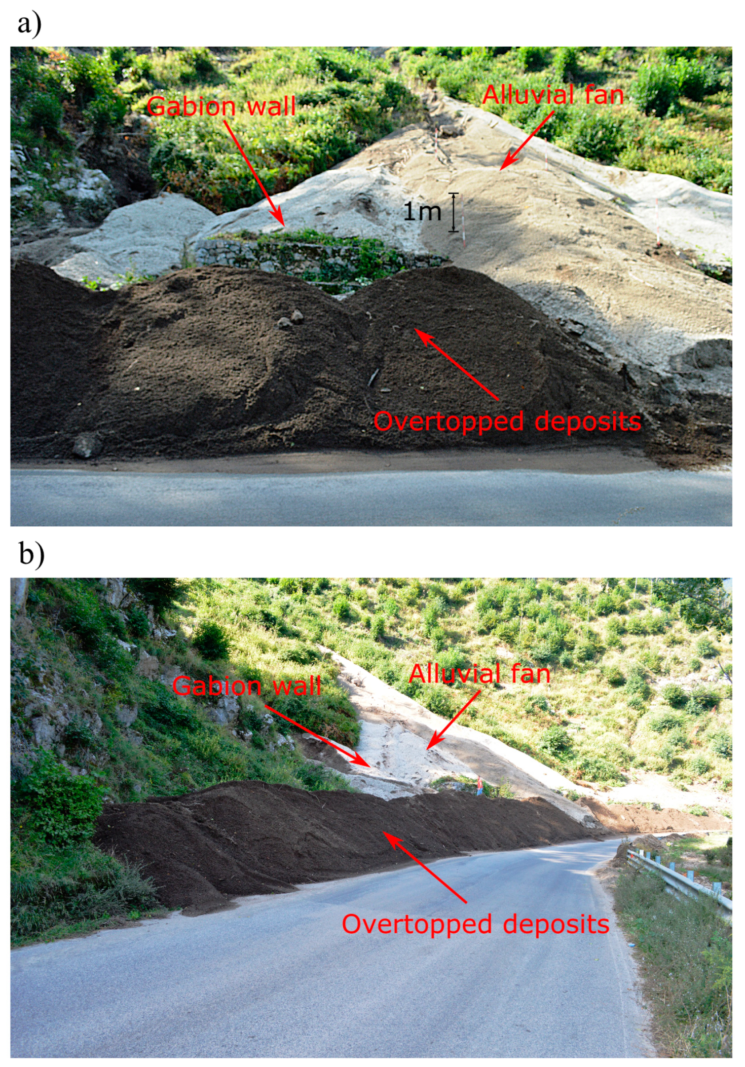
The DF area under study is characterized by frequent debris flow events running along a steep gully with an average inclination of ≈40°. At the lower end of the gully is an alluvial fan with a decreasing slope formed upstream a 30 m-long gabion wall, built to protect the road. It is worth mentioning that the deposition area upstream the gabion wall is not regularly emptied after DF events and, as a consequence, the available volume upstream the gabion wall is often smaller than the total volume of mobilized sediments during a single DF event. Therefore, in recent years a number of DF events partially overtopped the gabion wall and, consequently, hit the road. As an example, Figure 3 reports a picture of pumiceous deposits, taken soon after an event occurred in September 2014, which noticeably overtopped the gabion wall.
Heavy rainfalls are often capable of mobilizing the pyroclastic sediments lying on steep slopes and, consequently, cause shallow landslides that typically develop into DFs. The trigger mechanism of the collapses is probably due to a local increase of water pore pressure within the pumice layers, which causes local failures [41]. Conversely, the run-off depth of rain water is typically low owing to the high slopes and, thus, is unlikely to cause significant bed-load transport. In the site under study several DF events have been observed in the last decade. Nonetheless, a great amount of potentially unstable pumice deposits is still present in the upper part of the basin, indicating that the likelihood of further collapses is still very high.
This work focuses on the numerical reconstruction of a specific DF event, occurred on the 10th October 2013. This event was selected among the others, since we could gather detailed field surveys before and after it. During the event large volumes of pumiceous deposits moved from two niches, located about 120 m upstream of the gabion wall, at a relative elevation of ≈65 m above the road level. Henceforth, the two niches at the right and left sides of the gully will be referred to as N1 and N2, respectively. Satellite images, taken from Google Earth at different dates are reported in Figure 4, showing the evolution in time of N1 and N2.
During the DF event, the nearest rain gauge, located in the town centre of Tramonti (few kilometers South from the site), recorded a cumulative rainfall of 60 mm in 4 h with a maximum intensity of about 50 mm/h. Rainfall data were provided by the Regional Center of the Italian Civil Protection. However, since the elevation of the rain gauge is about 350 m below the site under study, it should be kept in mind that the gauge might slightly underestimate the actual rainfall occurred at the site under study, owing to the well-known orographic effects on the spatial variability of the rainfalls.
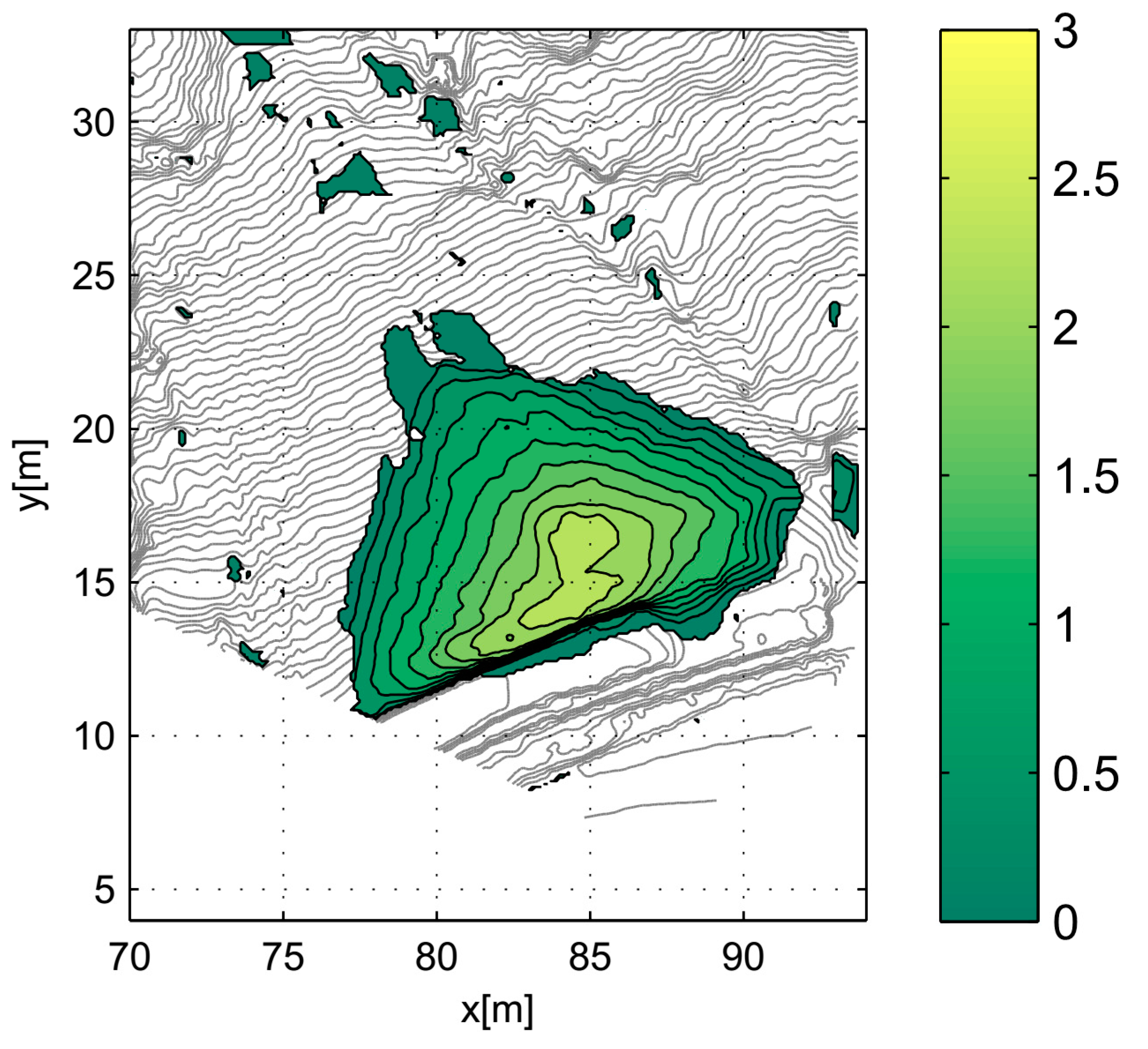
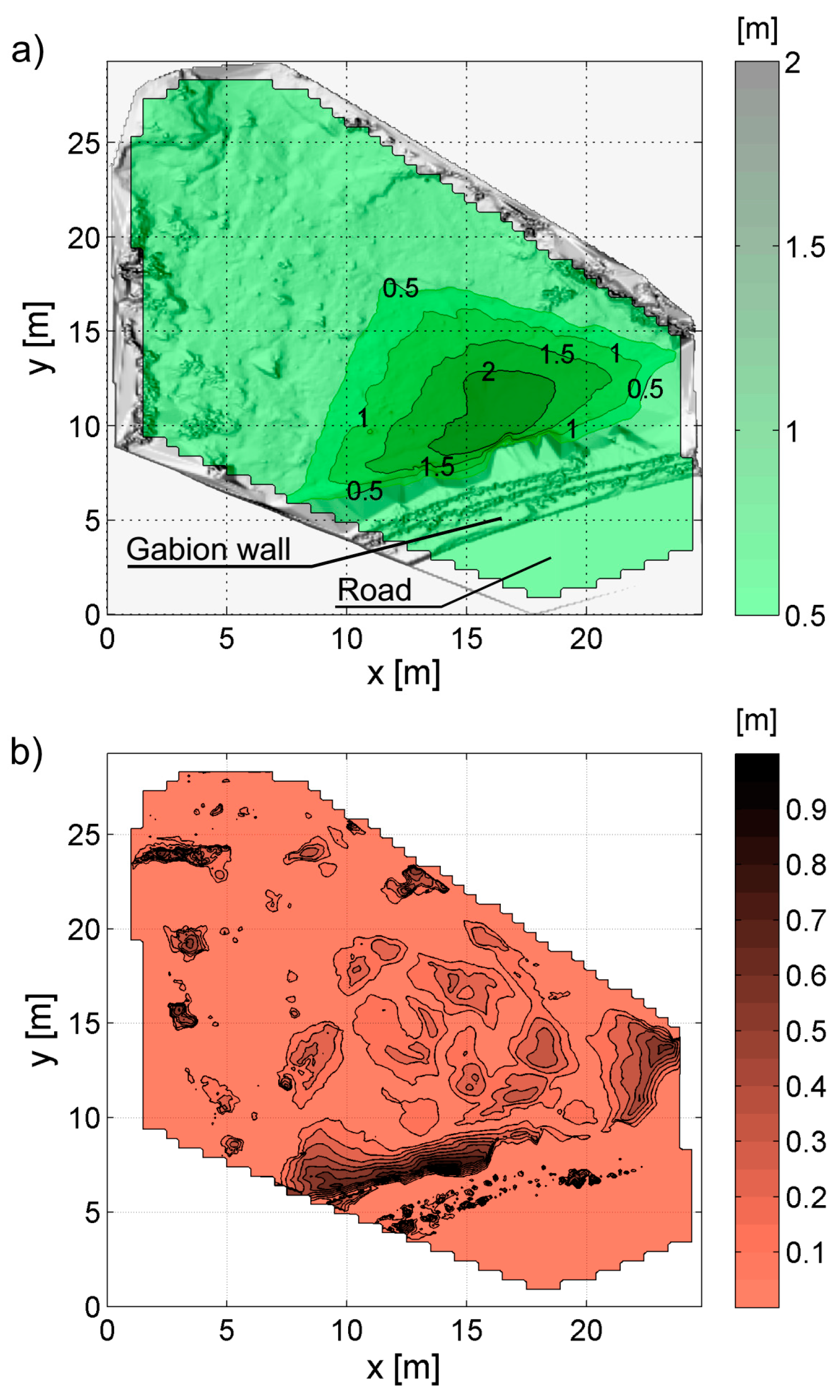
The collapses of pumice layers from the niches N1 and N2 gave place to a channelized DF along the gully that deposited upstream the gabion wall. By considering the relatively small magnitude of the rainfall, the smallness of the basin and the steep slope of the gully, it can be reasonably inferred that the run-off water depths were very small and, consequently, that the granular-liquid mixture was not saturated by water. As a consequence, it is reasonable to speculate that the buoyancy effects on pumice sediments and other complex hydrodynamic interactions between solid phase and interstitial fluid are negligible in this case. Apart from a small fraction of the total volume (of order of few cubic meters), the gabion wall was essentially not overtopped during this relatively small DF event. Such a circumstance allowed for a reasonably precise estimation of the total volume of the deposit behind the gabion wall, obtained by the comparison of two digital terrain models (DTM), taken before (27/06/2013) and after (18/10/2013) the event. The DTM were obtained by the terrestrial laser scanner (TLS) survey, employing the instrument TOPCON GLS-1500, and exhibit a very high resolution (of order of ≈1 cm), made possible thanks to the almost complete absence of vegetation inside the gully [30]. By comparing the two DTM, the volume of deposit was estimated equal to 146 m3. The shape of the deposit on the alluvial fan is reported in Figure 5. Based on field observations after the event, it was verified that the volume of deposit on the alluvial fan, i.e., upstream the wall, mainly came from the two niches (N1 and N2) located above, though minor amounts of granular material were eroded along the gully.
Differently, the DTM of the initiation and propagation zones was obtained by photo-modeling techniques applied to more than 160 aerial digital photographs taken in December 2013 through a UAV, equipped with a standard digital camera (model. Sony CX 260, manufacturer SONY–Tokyo, Japan). The average accuracy of this second survey is ≈10 cm. The pictures taken by the UAV were subsequently analyzed by the software Agisoft Photoscan (ver. 1.0.4), which is capable of yielding a high-resolution DTM through an image-based 3D-modelling algorithm. For more details about the photo-modeling survey technique we refer the Reader to our previous work [30].
Small natural leaves, made of coarse pumice material accumulated at the sides of the flow during the DF event could be observed inside the gully by post-event inspection. From this observation, it was possible to estimate a peak flow depth of 85 cm (with an uncertainty of ±15 cm), in a specific cross section, hereafter referred to as S1 and located few meters upstream the upper part of the alluvial fan.
3. Results
3.1. Preliminary Analysis for the Choice of the Resistance Law and Parameters Calibration
A first set of preliminary numerical simulations was performed in order to identify a proper flow resistance law and, subsequently, to calibrate its parameters. As the only constraint available for the calibration is the shape and the depth of deposit, initially we choose to simulate only the propagation and the deposition of the debris flow on the lower alluvial fan.
Analogous to that reported in [30], the input debris flow discharge at the upstream section, S1 (i.e., upper boundary condition) was assumed to be a one-surge triangular hydrograph. The volume of the hydrograph was set equal to the measured volume of deposit, 146 m3. The peak flow rate, set equal to 5.15 m3/s, was estimated by imposing the peak flow depth observed in the cross section S1 and assuming the occurrence of the hydraulic critical state. The time length of the hydrograph is 56.7 s. A sensitivity analysis on the peak flow depth, varied within its accuracy range (i.e., between 70 cm and 100 cm), was performed in [30]. It was found that the depths of deposit exhibit negligible variations in the investigated range of input hydrographs.
In this preliminary numerical simulations, the spatial domain was chosen to solely contain the debris fan, the gabion wall and some part of the road facing the gabions. The numerical simulations were performed on a basal topography, consisting of the pre-event DTM of 27/06/2013 obtained by TLS survey.
Various resistance laws were tried to reproduce the observed deposit. Owing to the coarse granulometry of the pumiceous material and non-negligible frictional effects, visco-plastic rheological laws (such as Bingham or Herschel-Bulkley laws), which are typically suitable for mud flows or fine-sediment pyroclastic debris flows [28], resulted totally inadequate in this case. In fact, these rheologies are unable to correctly reproduce non-null slopes in the final deposit. Much better results are obtained by employing the friction-collisional Voellmy model, which was historically proposed for describing the snow avalanches [31,32]. Several experimental studies available in literature show that this model is also able to describe granular flows and rock avalanches [42,43,44]. The Voellmy law, which cannot be viewed as a rigorous rheological model but more as a phenomenological resistance law, simply assumes that the basal shear stress, can be estimated as the sum of two terms, a rate-independent Coulomb friction term and a collisional turbulent-like term,
where α is the local inclination angle of the basal surface, h the flow depth, V the flow velocity and ρ the bulk density of the granular mixture. The two model’s parameters to be calibrated are: ϕ which represents a dynamic angle of friction depending on the angle of internal friction of the granular mixture; Cz, which can be viewed as a Chezy-like conveyance coefficient of dimensions [L1/2/T]. The angle of repose of the pumice granular material was experimentally estimated by freestanding cone method [45] at the LIDAM (Environmental and Maritime Hydraulics Laboratory of the University of Salerno) and is found to be 36° ± 2°. This measurement appears congruent with other data available in literature on similar pumice soils in Campanian area [39,40,41]. Yet, the dynamic angle of friction of the mixture of pumiceous material and water, to be used in Equation (2), is expected to be somehow smaller than this angle, due to the lubricating action of the interstitial fluid.
The optimal values of φ = 28.5° and Cz = 30 m1/2/s, were obtained by a back-analysis of the measured shape of deposit. The predicted deposit was found to be in sound agreement with the post-event DTM, showing an average absolute error of ≈0.08 m. The comparison between the numerically predicted deposit and the measured data is reported in Figure 6.
A more parsimonious resistance model, consisting of a simple Coulomb friction rate-independent resistance law with the assumption of isotropic normal stresses, was also tried. This model can be straightforwardly obtained from Equation (2), by simply removing the rate-dependent term. In this case, the sole parameter, φ, was optimized. We briefly report that, in this case, the best agreement between the numerical simulation and the field data is obtained with a slightly higher value of the angle of friction, φ = 32°, and the average absolute error resulted to be slightly larger (≈0.10 m). Although the degree of agreement with the measured deposit is still reasonably good and quite similar to the one found by using the Voellmy model, it is found that the Coulomb friction model tends to largely overestimate the flow velocities during the propagation stages, owing to the lack of a rate-dependent resistance term. Namely, a continuous and unrealistic acceleration of the avalanching mass is predicted on slopes higher than tan φ. Conversely, it can be speculated that the two resistance laws (Voellmy and pure Coulomb) perform similarly during the deposition stages because the rate-dependent momentum exchanges progressively fade away, as the granular mass slows down.
3.2. Numerical Simulations of the Pumice DF from Initiation to Deposit
When a mathematical-numerical model is used for describing a DF, large uncertainties are linked with the estimation of the input hydrograph or, generally speaking, of the initial conditions. In some cases the initial position of the mobilized mass is known or can be estimated with sufficient precision by field survey. Using this information, it is possible to perform numerical simulations of all the stages of the phenomenon from initiation to deposit [20], so that we are allowed to estimate not only the final shape of deposit but also the temporal evolution of the flow depths and velocities.
With reference to the investigated DF, here, we assume a sudden release of the pumice masses from niches, N1 and N2. This assumption is motivated by computational needs and it is also supported by field data. In fact, since by post-event surveys the crowns of the niches appear sharp and appear to have retrogressively moved, it is likely that the DF triggering occurred as a sudden local failure more than as a slow erosion process. From the mathematical and numerical viewpoint the considered failure mechanisms are totally analogous to the standard dam-break case of hydraulics.
In the absence of topographic data of the whole channel before the event, the numerical simulations were carried out by using the DTM, obtained by aerial survey of December 2013. It amounts to assuming that the topography along the gully did not change significantly during the investigated DF. Strictly speaking, this assumption might be inaccurate due to erosion/deposition processes. However, it should be noted that it is congruent with the employment of a mathematical model neglecting erosion/deposition processes along the flow path. Moreover, it should be kept in mind that the proper calibration of more sophisticated movable bed mathematical models would have been much more difficult, given the aforementioned lack of field data. The topography of the alluvial fan is given by the pre-event DTM of June 2013. The two DTMs, related to the alluvial fan and to the propagation channel, were merged together. A Gaussian filter (with standard deviation of 1.5 m) was employed at the boundaries of the debris fan, in order to properly smooth any artificial topographic jump and, thus, make the topography suitable for the subsequent numerical simulations.
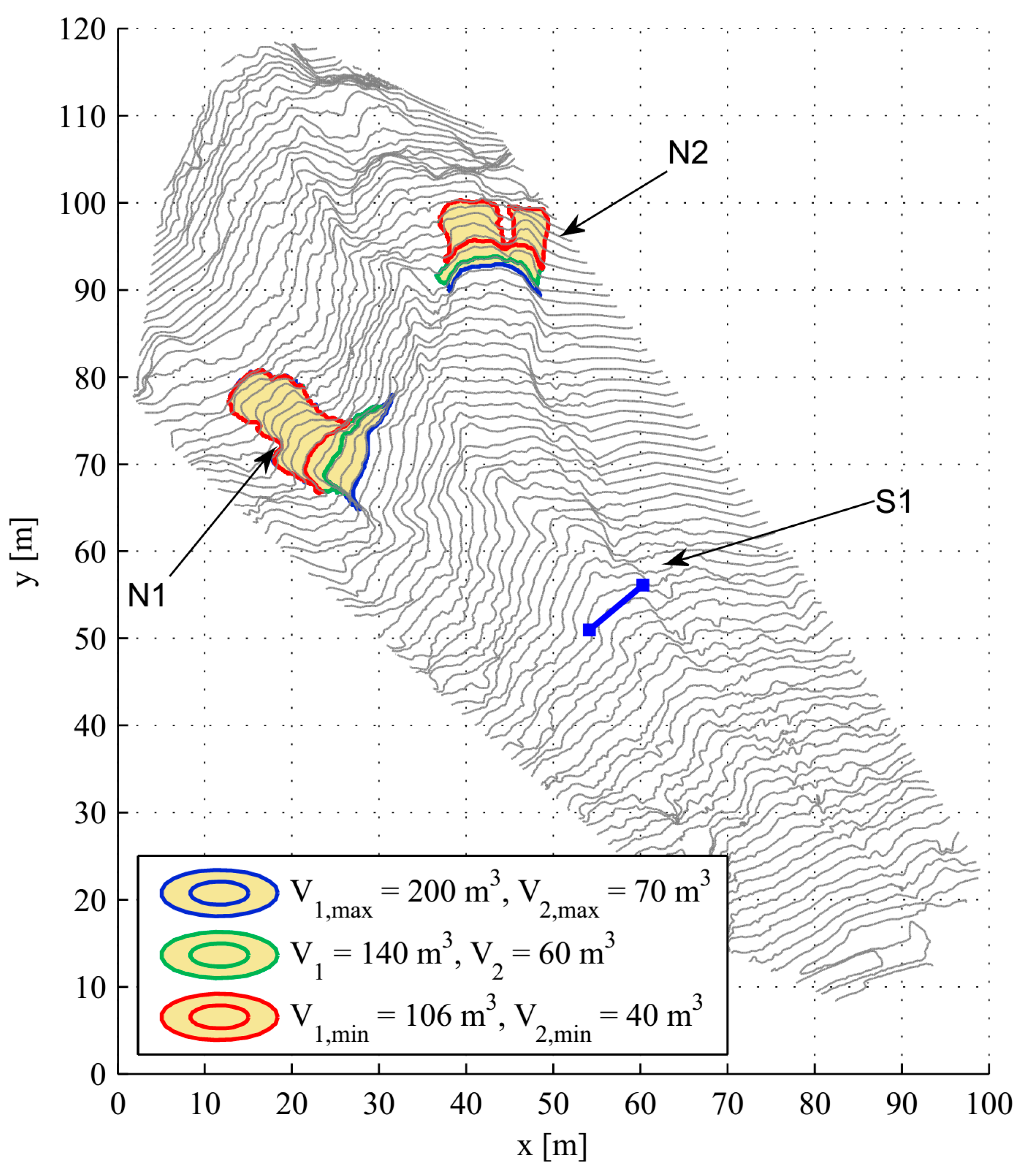
The initial depths of deposit in the two niches are reconstructed by interpolating the topography around the niches’ crowns, i.e., the neighbouring soil surface not involved in the collapses. Such a calculation is affected by some uncertainties mainly due to the fact that it was not possible to exactly determine the front positions of the mobilized volumes. From satellite images and the field survey of June 2013 it was revealed that the niche, N2, had been already partially collapsed at the moment of the investigated DF event of October 2013. Therefore, the majority of the mobilized volume is likely to have originated from the other niche, N1. By interpolation of the post-event topography and by comparison with the pre-event satellite images, the estimations of the volumes, mobilized from niches N1 and N2, are ≈140 m3 and ≈60 m3 respectively. The aforementioned uncertainties affecting these estimations are of order of few tens of cubic meters. The estimated volumes together with the related bands of uncertainties are reported in Figure 7.
No video-recording instrumentation is installed in the site under study; thus, the exact sequence of events during the triggering phases is unknown. In order to overcome this lack of knowledge, the following three different plausible scenarios were investigated:
- Scenario n. 1 (one dam-break wave): mobilization of the pumice deposits only from niche, N1;
- Scenario n. 2 (two dam-break waves merging together into a unique wave along the propagation channel): simultaneous mobilization of pumice deposits from niches N1 and N2;
- Scenario n. 3 (two subsequent dam-break waves): mobilization of pumice deposits from niche N1 and subsequent mobilization from niche N2.
In the third scenario, the second dam-break wave from N2 was numerically simulated by using as input topography the deposit distribution of the previous numerical simulation of the dam-break wave from N1. The other possible scenario, consisting of the initial mobilization of deposits from niche N2 and subsequent mobilization from niche N1, is not reported, because preliminary simulations revealed that it gives much worse results in terms of the shape of the final deposit. Moreover, it should be noted that the sub-basin of niche N2 is noticeably smaller than that of niche N1: thus, also from a hydrological viewpoint it is unlikely that the failure of N2 occurred before the failure of N1.
For each scenario, different numerical simulations were carried out by assuming various mobilized volumes from the two niches (within the related uncertainties, already shown in Figure 7). A complete list of the numerical simulations is reported in Table 1. Since the employed finite volume numerical scheme (HLLC) of FLATModel is of explicit type, the time steps in all simulations are calculated by imposing a CFL (Courant-Friedrichs-Lewy number) constraint equal to 0.5. The parameters employed in the Voellmy resistance law, (2), are: φ = 28.5° and Cz = 30 m1/2/s, as reported in Section 3.1. In order to quantitatively assess the degree of agreement between the numerical simulation and the field measurements, the following L1-type normalized error index e.g., [22] is employed
In Equation (3) the summations extend over the cells of the discretized spatial domain, where both the predicted flow depth, hsim,i, and the measured flow depth, hmeasured,i, are available. Thus, the error index could be calculated on the alluvial fan where pre- and post-event DTMs were available. Furthermore, the mean of the absolute error (expressed in meters), Ē, and the 90th percentile, E90%, of its distribution over the alluvial fan are also reported in Table 1, together with the numerically predicted volume of deposit on the fan, Vdep. Please note that this volume is always smaller than the total volume, assumed to be collapsed from the niches in the numerical simulation, since a portion of it stopped along the propagation channel due to local variations of the basal slope and another small portion occasionally may have overtopped the gabion wall.
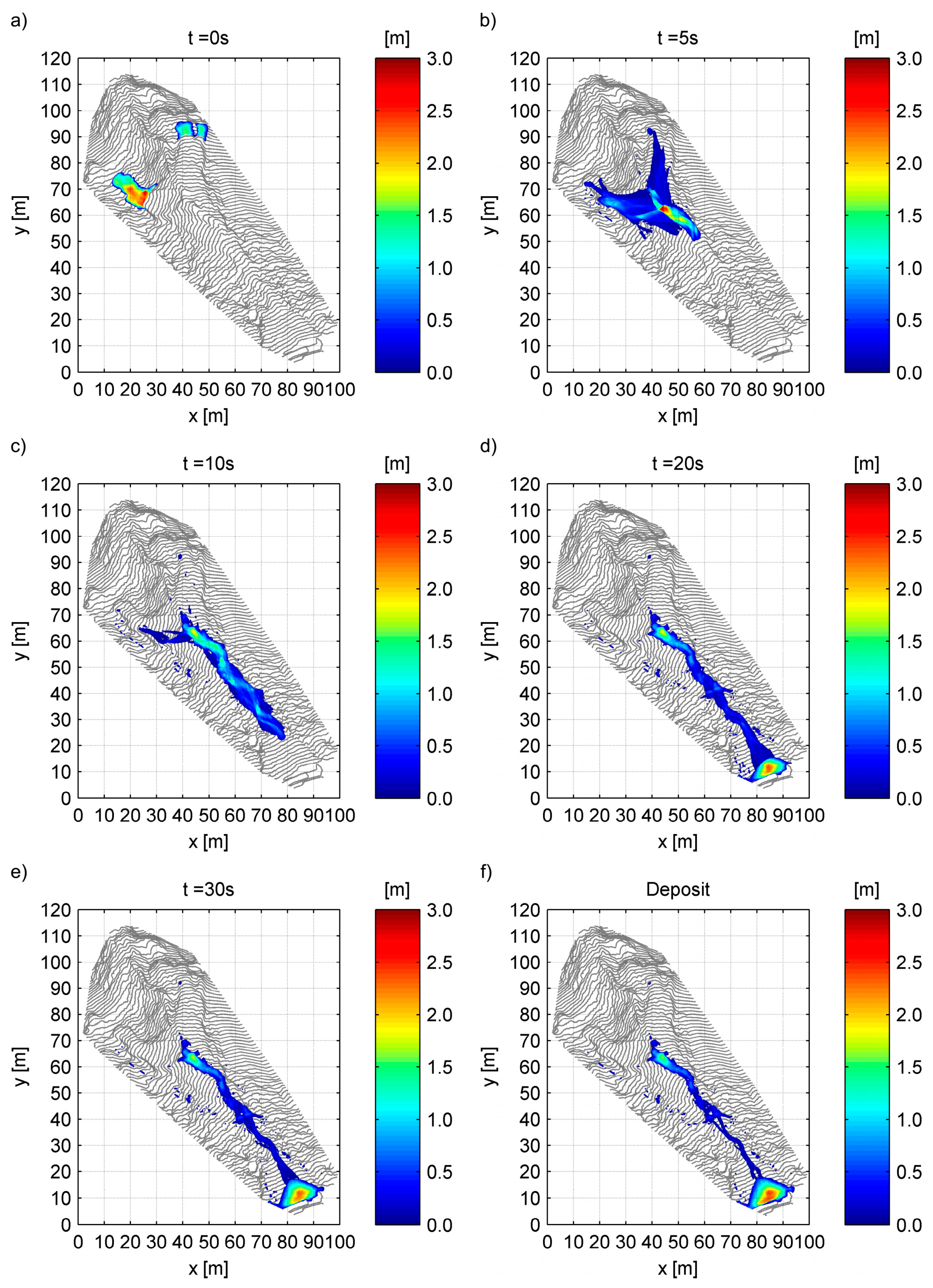
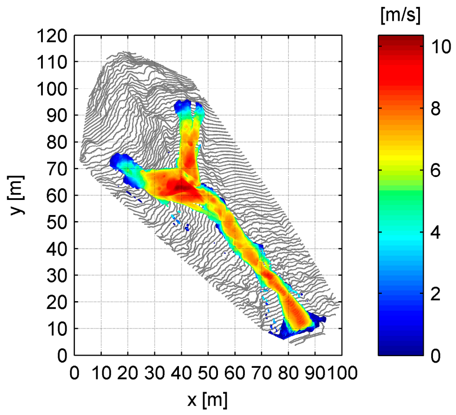
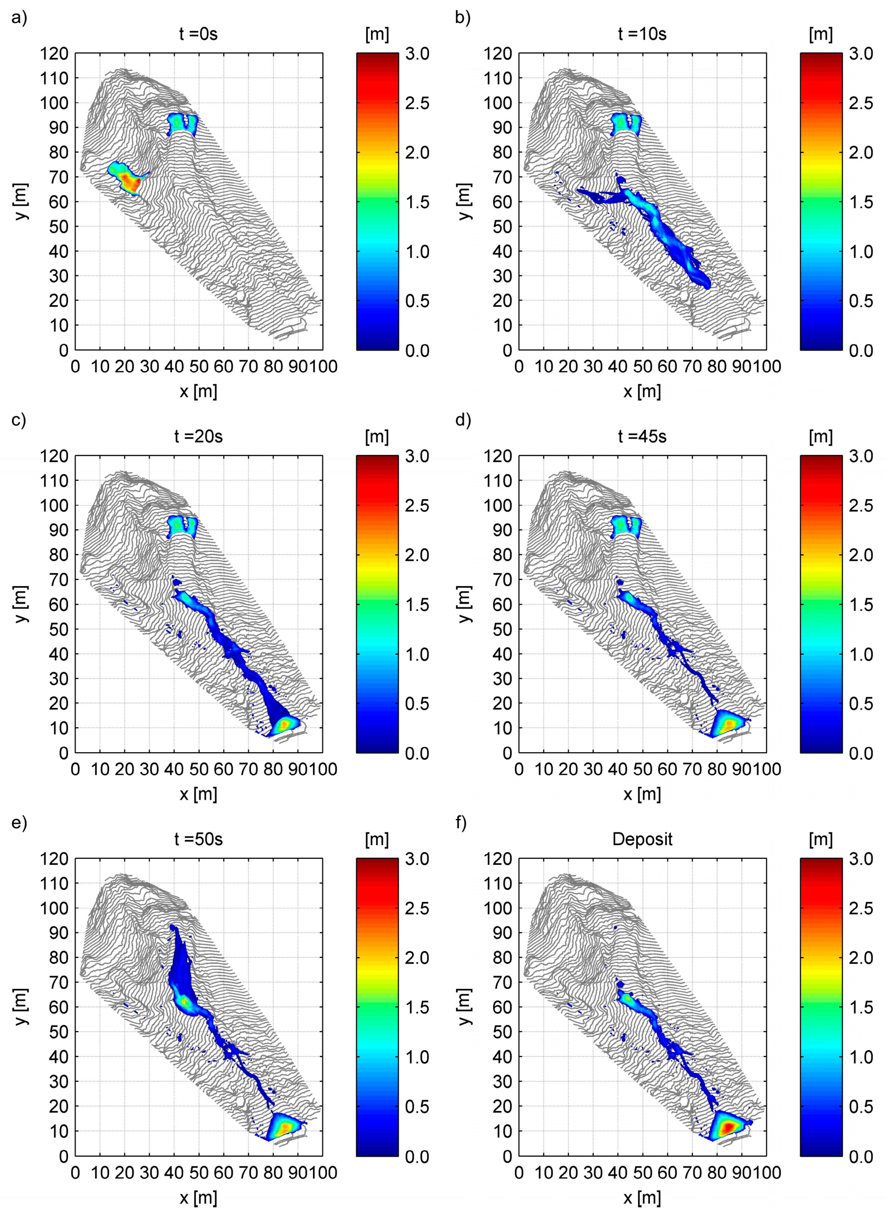
Before presenting the best-fitting simulation for each scenario, it can be observed from Table 1 that the average error of the deposit height in the debris fan is always smaller than 10 cm for all the investigated numerical simulations. This corroborates the robustness of the modelling approach and, especially, the suitability of the chosen resistance law. In Scenario 1, the best agreement is obtained by the simulation SIM-1-4, in which a volume of 180 m3 moves from niche N1. The agreement with the measured shape of deposit is reasonably good with a normalized error index Enorm = 0.222 and the average absolute error, Ē, slightly below 7 cm. Yet, it should be noted that the predicted volume of deposit 133 m3 is 9% smaller than the value measured by TLS survey (146 m3). As mentioned above, the reason of this discrepancy is partly due to the fact that a fraction of the released volume from niche N1 stops along the gully, and partly due to some minor overtopping beyond the gabion wall. The agreement with the field measurements further increases in the other two scenarios. In Scenario 2, the best correspondence with the survey data is obtained by simulation, SIM-2-5, where a volume of 150 m3 coming from niche N1 and a volume of 40 m3 coming from niche N2 are released simultaneously. The average absolute error, Ē, and Enorm are quite similar to the optimal simulation of Scenario 1, whereas Vdep=137m3 exhibits a better agreement with the measured volume of deposit. With reference to the optimal simulation SIM-2-5 of Scenario 2, the evolution of the flow depths over time in the whole spatial domain is reported in Figure 8. In the same figure the final deposit, observed when the entire flow reaches a state of rest at t ≈ 45 s after the initiation, is also reported (Figure 8f). Moreover, the envelope of the maximum of the velocity modulus, , of SIM-2-5 is shown in Figure 9. The peak flow velocity, predicted by the numerical simulation, is slightly larger than 10 m/s. We report that also in the other numerical simulations the peak velocity is found to be of the same order.
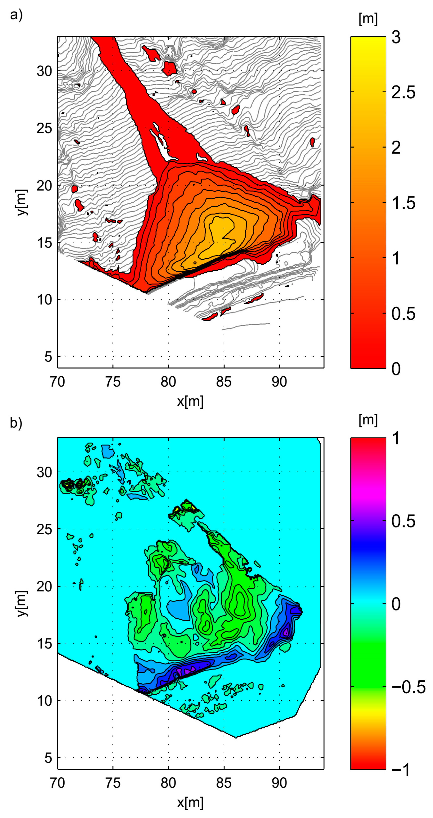
The shape of deposit on the alluvial fan, predicted by SIM-2-5, is reported in Figure 10 together with the error, hsim,I − hmeasured,i, calculated with respect to the surveyed data (Figure 10b). As shown in Figure 10b, it should be noted that, though the triangle-like shape of deposit is correctly predicted by the mathematical model, the numerical simulation tends to overestimate the deposit depth immediately behind the gabion wall and, conversely, it slightly underestimates it in the upper zone of the alluvial fan. This limitation of the numerical simulation will be discussed in more detail in Section 4.
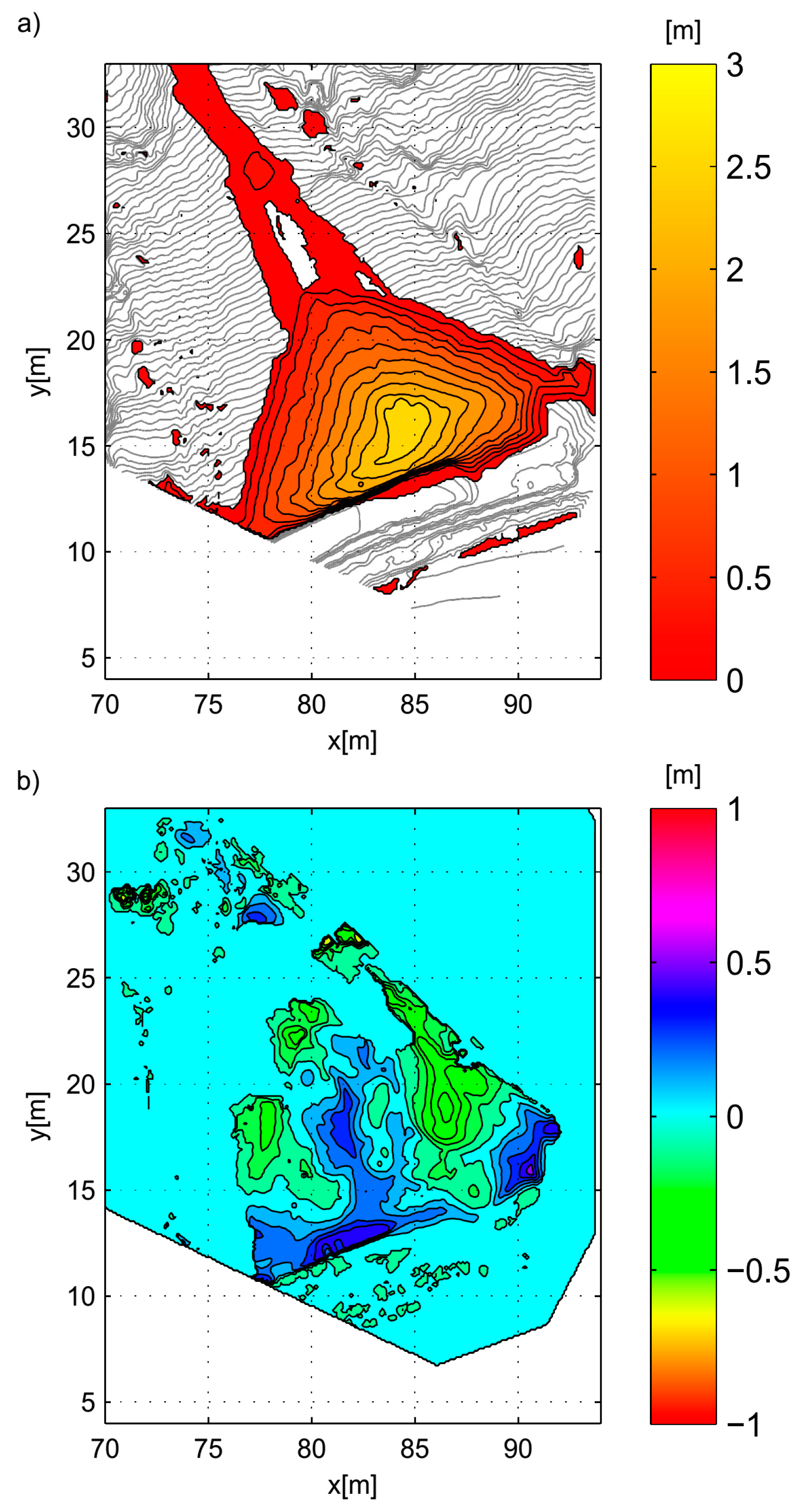
Now, let us present the numerical simulations related to Scenario 3, involving two subsequent dam-break waves from niches N1 and N2. The best agreement with the measured deposit is obtained by the simulation, SIM-3-2, in which the volumes of 140 m3 and 50 m3 are released from niches N1 and N2, respectively. In this case the error indicators are even slightly smaller than Scenario 2: Ē = 0.064 m and Enorm = 0.208. The evolution of flow depths over time is reported in Figure 11. It should be noted that, in this case, the time length of the DF event is larger (≈90 s) than that of Scenario 2, due to the hypothesis of two subsequent dam-break waves. Figure 12 reports the shape of predicted deposit on the alluvial fan and the error on the flow depths. As shown by Figure 12b, the systematic overestimation of the flow depth immediately behind the gabion wall is noticeably reduced compared to the optimal simulation of Scenario 2 (SIM-2-5). This numerical result appears as the most realistic among all three investigated scenarios.
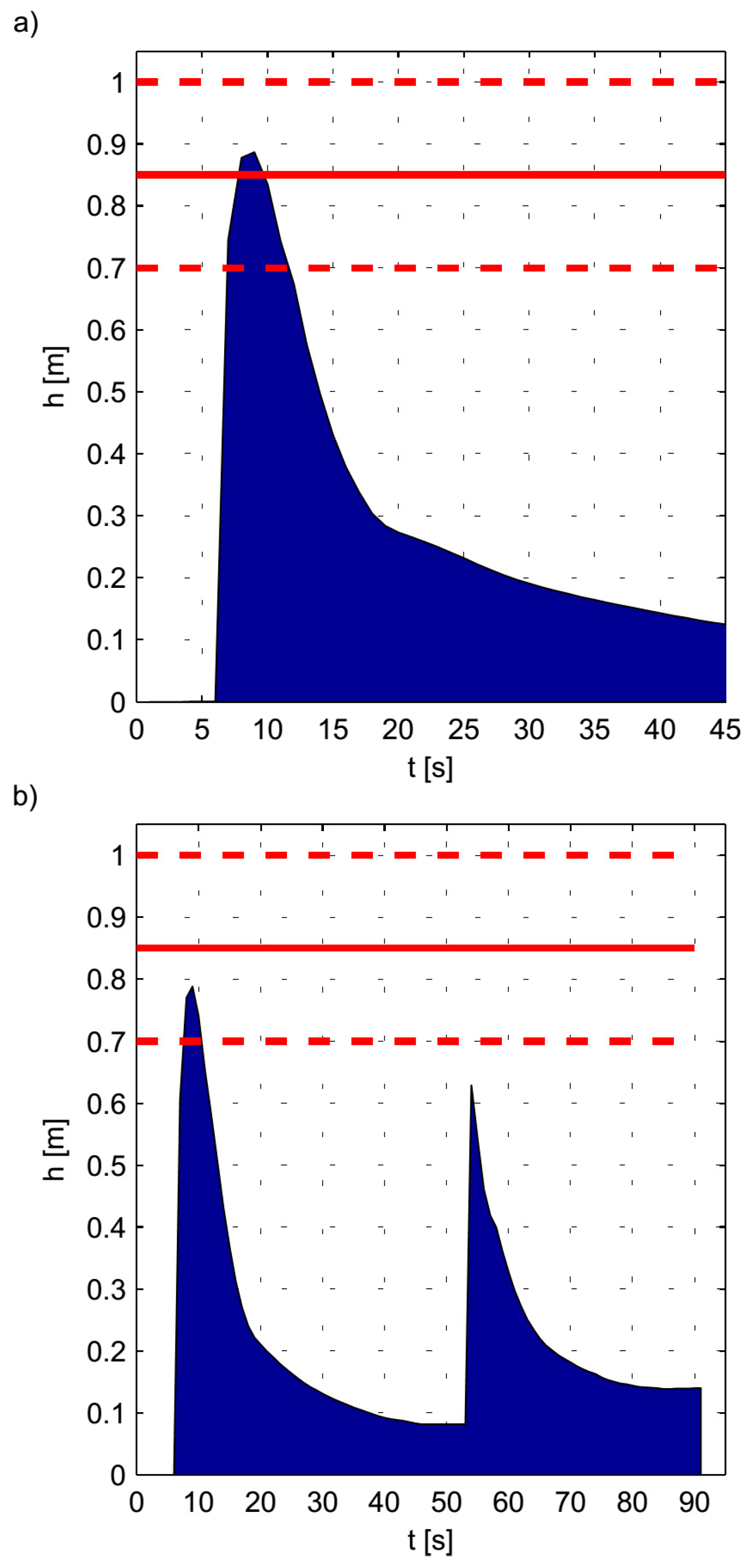
Finally, the evolutions of the flow depth, obtained by the optimal numerical simulations, SIM-2-5 and SIM-3-2, at the cross section S1 are reported in Figure 13. The numerically predicted flow depths could be also compared with the measured peak flow at the same cross section, S1. The agreement is reasonably good in both cases, since the predicted peak lies within the uncertainty range of the measured peak flow depth 85 cm ± 15 cm.
4. Discussion
This paper focused on the numerical reconstruction of pumiceous DF. The proposed integrated approach employs the shallow-water code, FLATModel, which is specifically designed for describing the DF propagation over irregular topographies and could be preliminarily calibrated by means of field data, obtained from TLS and photo-modelling aerial surveys. In the calibration stage, reported in Section 3.1, different rheological laws were tried. It emerged that classical rheological laws, such as Bingham and Herschel-Bulkley laws, which are typically suitable for mud flows and fine-sediment pyroclastic debris flows [28], are completely inappropriate in the case of pumice DFs. Indeed, they are found to be unable to capture non-null slopes of the deposit in the alluvial fan. Conversely, the Voellmy resistance law [31,32] was identified as the most suitable approach. This finding strongly indicates that the investigated pumiceous DFs exhibit a granular behaviour, where the main momentum exchange mechanisms are represented by friction and collisions among grains e.g., [10,25]. In this regard, a pumiceous DF generally behaves as a stony debris flow, at least as long as the run-off water depths are small enough so that buoyancy effects remain negligible. In nature this normally occurs when the topography slopes are sufficiently high. A first result of the present numerical investigation is that the complex lubricating and drag effects of the interstitial fluid can be approximately accounted for in the dynamical angle of friction of the Voellmy Expression (2), which is found to be few degrees (≈7.5°) smaller than the angle of repose of the granular material.
In order to reconstruct the investigated DF event from initiation to deposit, the code FLATModel was subsequently run over different plausible dam-break scenarios. The results reported in Section 3.2 (cf. Table 1 and Figure 8, Figure 9, Figure 10, Figure 11 and Figure 12), indicate that, regardless of the specific assumption about the triggering mechanism, the numerical simulations using the calibrated Voellmy resistance law yield a sound agreement with the post-event field data (with an average error always smaller than 10 cm). The envelope of the flow velocities along the propagation channel (cf. Figure 9), predicted by the numerical model, are of order of 10 m/s in all scenarios. Considering the relatively small length of the gully, the predicted magnitude of the flow velocities appears realistic and also congruent with other field data of granular DFs available in literature, e.g., [18,20,46]. Moreover, it is worth underlining that much worse estimations of the flow velocities were obtained by employing a rate-independent resistance law, such as the Coulomb friction law [17,24,25,30]. In fact, owing to the lack of a rate-dependent term, unrealistic accelerations of the granular flow are systematically observed whenever the topography slopes are higher than the angle of friction employed in the resistance law. The suitability of the proposed modelling approach and, specifically, of the Voellmy resistance law is also confirmed by the good agreement between the peak flow depth predicted by numerical simulation in the various scenarios and the maximum flow depth measured at the cross section S1 (cf. Figure 13).
The best quantitative agreement between the numerical simulation and post-event field data is obtained in the third scenario with the simulation SIM-3-2 (Figure 11 and Figure 12), exhibiting an average error of the deposit of Ē = 0.064 m. By comparing the best numerical simulations obtained from different dam-break scenarios, we observed that the first two scenarios (characterized by a single triggering event) systematically overestimate the depth of the deposit immediately behind the gabion wall and, conversely, slightly underestimate it in the upper zone of the alluvial fan (cf. Figure 10b). This discrepancy probably arises because the granular material reaches the debris fan with an overestimated kinetic energy, which also provokes some minor overtopping beyond the wall. This could be due to the fact that a single dam-break wave takes place in Scenario 1, and also in Scenario 2 an almost unique wave along the main propagation channel emerges from the simplifying assumption of simultaneous collapses from both niches (i.e., one single triggering event). Also, the simplistic assumptions of the Voellmy model, in particular that of a constant angle of friction during the deposition process, which obviously cannot take into account the hysteretic behaviour of granular media near the state of rest [47], could affect the model capability of properly describing the final stages of the flow. Moreover, it should be underlined that FLATModel tries to capture the avalanche stop, by calculating the slowdown of the flow in each computational cell of the fixed topography. In reality a progressive depositional process occurs. Indeed, owing to gravity, the deposition process of a granular mixture typically takes place in a stratified fashion, where the lower layers progressively come to rest well before the upper surface flow, which exhibits larger flow velocities conversely [48,49]. Such a progressive stop causes variations in time of the topography of the alluvial fan, which in turn could influence the flow dynamics. To properly describe the complex dynamics of the depositional processes, classical shallow water models could be improved by means of two-layer/multi-layer, e.g., [49,50,51], and movable-bed approaches, e.g., [52,53,54], which, however, generally require the calibration of a greater number of parameters. It was interesting to note that the best simulation in Scenario 3 (SIM-3-2) partially overcomes the aforementioned limitations of the numerical reconstruction at the deposition stages. We believe that this result could be obtained thanks to the assumption of two subsequent dam-break waves, of which the second one moves on the updated topography resulting from the first dam-break flow. For the reasons highlighted above, it is not surprising that a tangible improvement is obtained at the deposition stages, thanks to the employment of an updated topography after the first dam-break wave. These observations indicate the direction of further numerical research, possibly involving more sophisticated mathematical modelling approaches. However, it should be kept in mind that, as the number of model parameters increases, also the resolution and accuracy of field data should be consequently improved, so as to properly calibrate them. In this regard, the field surveys, and, in particular, the cost-effective photo-modelling techniques represent exceptionally useful tools for further modelling attempts.
5. Conclusions
In order to map the risk associated with debris flows and design proper mitigation measures, it is necessary to implement a methodology capable of providing reliable predictions with the data usually available in practical cases. The integrated approach developed here is based on the implementation of a shallow water mathematical model in which the triggering mechanism and the dynamic behaviour of the flowing mixture are determined by back-analysis of field data. A case study of pumice debris flow, occurred in the Amalfi Coast (Italy), is investigated. Numerical simulations were performed by employing the depth-averaged mathematical-numerical code, FLATModel, which is based on the shallow-water equations written in curvilinear coordinates and is specifically designed for describing the propagation of debris flows over irregular mountainous topographies. The topography of the area and the field data, necessary for the back analysis, are obtained through innovative and cost-effective survey techniques: the topography of the area, before and after the event, was obtained by terrestrial laser scanner and photo-modelling surveys. This latter technique is capable of providing DTMs with reasonably high spatial resolution, in an inexpensive and time effective way. The pre- and post-event DTMs allowed for the estimation of the deposited volume and the geomorphological evolution of the initiation areas.
The back-analysis reveals that the pumice DFs exhibit a granular-flow behaviour, which can be well captured by a frictional-collisional resistance law of the Voellmy type. The numerical results showed a reasonably good capacity of the model to describe the shape and slope of the deposit. Moreover, different from a simple Coulomb friction resistance law, the Voellmy model is also capable of realistically describing the velocity field along the propagation channel, thanks to the presence of a rate-dependent term.
The comparison among different triggering scenarios of dam-break type showed that the uncertainties on the actual temporal sequence of different mass releases are not particularly crucial for the prediction of the final deposit. Indeed, in all the reported scenarios, the simulation captured the deposit with an average error always smaller than 10 cm. Nevertheless, the comparison showed that the best results are obtained under the assumption of two subsequent dam-break waves. This finding is probably due to the fact that, in this case, the second dam-break wave is numerically modelled on an updated topography, taking into account the propagation and subsequent stop of the first dam-break wave. In this way, the depositional processes could be more realistically described than in the other two scenarios, characterized by one single dam-break wave moving on a rigid bed topography.
Overall, we can conclude that the integration of innovative and cost-effective monitoring tools with hydraulic modelling tools is extremely promising for the prediction and mapping of debris flow deposits. Further developments may be achieved by performing multiple photo-modelling surveys separated by shorter time intervals, so as to better capture the terrain evolution. Thanks to these data unavailable until recently, it would become affordable also to calibrate and validate more sophisticated movable-bed or multi-layer shallow water models, involving a greater number of parameters.
Author Contributions
M.N.P. and L.S. conceived the research topic. F.S.V. carried out the numerical simulations with the supervision of L.S. and V.M., L.S. wrote the manuscript, while M.N.P. reviewed it.
Funding
This research received no external funding.
Acknowledgments
The authors thank N. Immediata for assistance during the laboratory tests on pumice, carried out at the LIDAM (Environmental and Maritime Hydraulics Laboratory of the Salerno University). The authors are grateful to the Survey Unit of the Dept. of Civil Engineering of the Univ. of Salerno (Italy) for the TLS and UAV surveys, previously performed in the framework of the Master’s thesis of M. Limongiello.
Conflicts of Interest
The authors declare no conflict of interest to disclose.
References
- Jakob, M.; Hungr, O.; Jakob, D.M. Debris-Flow Hazards and Related Phenomena; Springer: Berlin, Germany, 2005. [Google Scholar]
- Takahashi, T. Debris Flow: Mechanics, Prediction and Countermeasures, 2nd ed.; CRC Press: London, UK, 2014. [Google Scholar]
- Rickenmann, D. Debris-flow hazard assessment and methods applied in engineering practice. Int. J. Eros. Control Eng. 2016, 9, 80–90. [Google Scholar] [CrossRef]
- Midi, G.D.R. On dense granular flows. Eur. Phys. J. E 2004, 14, 341–365. [Google Scholar] [CrossRef] [PubMed] [Green Version]
- Carravetta, A.; Fecarotta, O.; Martino, R.; Sabatino, C. Assessment of rheological characteristics of a natural Bingham-plastic mixture in turbulent pipe flow. J. Hydraul. Eng. 2010, 136, 820–825. [Google Scholar] [CrossRef]
- Sheng, L.T.; Kuo, C.Y.; Tai, Y.C.; Hsiau, S.S. Indirect measurements of streamwise solid fraction variations of granular flows accelerating down a smooth rectangular chute. Exp. Fluids 2011, 51, 1329. [Google Scholar] [CrossRef]
- Carravetta, A.; Conte, M.C.; Fecarotta, O.; Martino, R. Performance of slurry flow models in pressure pipe tests. J. Hydraul. Eng. 2015, 142, 06015020. [Google Scholar] [CrossRef]
- Sarno, L.; Carravetta, A.; Tai, Y.C.; Martino, R.; Papa, M.N.; Kuo, C.-Y. Measuring the velocity fields of granular flows—Employment of a multi-pass two-dimensional particle image velocimetry (2D-PIV) approach. Adv. Powder Tech. 2018. [Google Scholar] [CrossRef]
- Sarno, L.; Papa, M.N.; Villani, P.; Tai, Y.-C. An optical method for measuring the near-wall volume fraction in granular dispersions. Granul. Matter 2016, 18, 80. [Google Scholar] [CrossRef]
- Sarno, L.; Carleo, L.; Papa, M.N.; Villani, P. Experimental investigation on the effects of the fixed boundaries in channelized dry granular flows. Rock Mech. Rock Eng. 2018, 51, 203–225. [Google Scholar] [CrossRef]
- Luna, B.Q.; Remaître, A.; Van Asch, T.W.; Malet, J.P.; Van Westen, C.J. Analysis of debris flow behavior with a one dimensional run-out model incorporating entrainment. Eng. Geol. 2012, 128, 63–75. [Google Scholar] [CrossRef]
- Berti, M.; Simoni, A. DFLOWZ: A free program to evaluate the area potentially inundated by a debris flow. Comput. Geosci. 2014, 67, 14–23. [Google Scholar] [CrossRef]
- Hürlimann, M.; McArdell, B.W.; Rickli, C. Field and laboratory analysis of the runout characteristics of hillslope debris flows in Switzerland. Geomorphology 2015, 232, 20–32. [Google Scholar] [CrossRef] [Green Version]
- Chae, B.G.; Park, H.J.; Catani, F.; Simoni, A.; Berti, M. Landslide prediction, monitoring and early warning: A concise review of state-of-the-art. Geosci. J. 2017, 21, 1033–1070. [Google Scholar] [CrossRef]
- Coviello, V.; Capra, L.; Vázquez, R.; Márquez-Ramírez, V.H. Seismic characterization of hyperconcentrated flows in a volcanic environment. Earth Surf. Proc. Land. 2018. [Google Scholar] [CrossRef]
- Capra, L.; Sulpizio, R.; Márquez-Ramirez, V.H.; Coviello, V.; Doronzo, D.M.; Arambula-Mendoza, R.; Cruz, S. The anatomy of a pyroclastic density current: The 10 July 2015 event at Volcán de Colima (Mexico). Bull. Volcanol. 2018, 80, 34. [Google Scholar] [CrossRef]
- Savage, S.B.; Hutter, K. The motion of a finite mass of granular material down a rough incline. J. Fluid Mech. 1989, 199, 177–215. [Google Scholar] [CrossRef]
- Iverson, R.M. The physics of debris flows. Rev. Geophys. 1997, 35, 245–296. [Google Scholar] [CrossRef] [Green Version]
- Fraccarollo, L.; Papa, M.N. Numerical simulation of real debris-flow events. Phys. Chem. Earth Part B 2000, 25, 757–763. [Google Scholar] [CrossRef]
- Medina, V.; Hürlimann, M.; Bateman, A. Application of FLATModel, a 2D finite volume code, to debris flows in the northeastern part of the iberian peninsula. Landslides 2008, 5, 127–142. [Google Scholar] [CrossRef]
- Sarno, L.; Martino, R.; Papa, M.N. Discussion of “Uniform flow of modified bingham fluids in narrow cross sections” by Alessandro Cantelli. J. Hydraul. Eng. 2011, 137, 621–621. [Google Scholar] [CrossRef]
- Sarno, L.; Carravetta, A.; Martino, R.; Tai, Y.-C. The pressure coefficient in dam-breaks flows of dry granular matter. J. Hydraul. Eng. 2013, 139, 1126–1133. [Google Scholar] [CrossRef]
- De Saint-Venant, A.B. Théorie du mouvement non permanent des eaux, avec application aux crues des rivières et à l’introduction des marées dans leurs lits. C. R. Acad. Sci. 1871, 73, 148–154. [Google Scholar]
- Savage, S.B.; Hutter, K. The dynamics of avalanches of granular materials from initiation to run-out. Acta Mech. 1991, 86, 201–223. [Google Scholar] [CrossRef]
- Gray, J.M.N.T.; Wieland, M.; Hutter, K. Gravity driven free surface flow of granular avalanches over complex basal topography. Proc. R. Soc. Lond. A 1999, 455, 1841–1874. [Google Scholar] [CrossRef]
- Sarno, L.; Papa, M.N.; Martino, R. Dam-break flows of dry granular materials on gentle slopes. In Proceedings of the 5th International Conference on Debris-Flow Hazards Mitigation: Mechanics, Prediction and Assessment, Padova, Italy, 14–17 June 2011; pp. 503–512. [Google Scholar]
- Laigle, D.; Coussot, P. Numerical modelling of mudflows. J. Hydraul. Eng. 1997, 123, 617–623. [Google Scholar] [CrossRef]
- Martino, R.; Papa, M.N. Variable-Concentration and boundary effects on debris flow discharge predictions. J. Hydraul. Eng. 2008, 134, 1294–1301. [Google Scholar] [CrossRef]
- Medina, V. Debris Flows and General Steep Slope Shallow Water Flows Numerical Simulation. Ph.D. Thesis, UPC, Barcellona, Spain, 2010. [Google Scholar]
- Papa, M.N.; Sarno, L.; Ciervo, F.; Barba, S.; Fiorillo, F.; Limongiello, M. Field surveys and numerical modeling of pumiceous debris flows in Amalfi Coast (Italy). Int. J. Eros. Control Eng. 2016, 9, 179–187. [Google Scholar] [CrossRef]
- Voellmy, A. Uber die Zerstörungskraft von Lawinen. Schweiz. Bauztg. 1955, 73, 212–217. [Google Scholar]
- Bartelt, P.; Salm, B.; Gruber, U. Calculating dense-snow avalanche runout using a Voellmy-fluid model with active/passive longitudinal straining. J. Glaciol. 1999, 45, 242–254. [Google Scholar] [CrossRef]
- Bouchut, F.; Westdickenberg, M. Gravity driven shallow water models for arbitrary topography. Comm. Math. Sci. 2004, 2, 359–389. [Google Scholar] [CrossRef] [Green Version]
- Pudasaini, S.; Wang, Y.; Hutter, K. Rapid motions of free-surface avalanches down curved and twisted channels and their numerical simulation. Philos. Trans. R. Soc. A 2005, 363, 1551–1571. [Google Scholar] [CrossRef] [PubMed]
- Toro, E.F.; Spruce, M.; Speares, W. Restoration of the contact surface in the Harten-Lax-van Leer Riemann Solver. Shock Waves 1994, 4, 25–34. [Google Scholar] [CrossRef]
- Cascini, L.; Ferlisi, S.; Vitolo, E. Individual and societal risk owing to landslides in the Campania region (Southern Italy). Georisk 2008, 2, 125–140. [Google Scholar] [CrossRef]
- Papa, M.N.; Trentini, G.; Carbone, A.; Gallo, A. An integrated approach for debris flow hazard assessment—A case study on the Amalfi Coast–Campania, Italy. In Proceedings of the 5th International Conference on Debris-Flow Hazards Mitigation: Mechanics, Prediction and Assessment, Padova, Italy, 14–17 June 2011. [Google Scholar]
- Papa, M.N.; Medina, V.; Ciervo, F.; Bateman, A. Derivation of critical rainfall thresholds for shallow landslides as a tool for debris flow early warning systems. Hydrol. Earth Syst. Sci. 2013, 17, 4095–4107. [Google Scholar] [CrossRef] [Green Version]
- Fiorillo, F.; Wilson, R.C. Rainfall induced debris flows in pyroclastic deposits, Campania (southern Italy). Eng. Geol. 2004, 75, 263–289. [Google Scholar] [CrossRef]
- Iamarino, M.; Terribile, F. The importance of andic soils in mountain ecosystems: A pedological investigation in Italy. Eur. J. Soil Sci. 2008, 59, 1284–1292. [Google Scholar] [CrossRef]
- Crosta, G.B.; Dal Negro, P. Observations and modelling of soil slip-debris flow initiation processes in pyroclastic deposits: The Sarno 1998 event. Nat. Hazard Earth Syst. 2003, 3, 53–69. [Google Scholar] [CrossRef]
- Hungr, O.; Evans, S.G. Rock avalanche runout prediction using a dynamic model. In Proceedings of the 7th. International Symposium on Landslides, Trondheim, Norway, 17–21 June 1996; Volume 11, pp. 233–238. [Google Scholar]
- Rickenmann, D.; Koch, T. Comparison of debris flowmodeling approaches. In Proceedings of the 1st International Conference on Debris-Flow Hazards Mitigation: Mechanics, Prediction and Assessment, San Francisco, CA, USA, 7–9 August 1997; pp. 576–585. [Google Scholar]
- Hürlimann, M.; Rickenmann, D.; Medina, V.; Bateman, A. Evaluation of approaches to calculate debris-flow parameters for hazard assessment. Eng. Geol. 2008, 102, 152–163. [Google Scholar] [CrossRef]
- Miura, K.; Maeda, K.; Toki, S. Method of measurement for the angle of repose of sands. Soils Found. 1997, 37, 89–96. [Google Scholar] [CrossRef]
- Hungr, O.; Evans, S.G.; Hutchinson, I. A Review of the Classification of Landslides of the Flow Type. Environ. Eng. Geosci. 2001, 7, 221–238. [Google Scholar] [CrossRef]
- Pouliquen, O. Scaling laws in granular flows down rough inclined planes. Phys. Fluids 1999, 11, 542–548. [Google Scholar] [CrossRef]
- Crosta, G.B.; Imposimato, S.; Roddeman, D. Numerical modeling of 2-D granular step collapse on erodible and nonerodible surface. J. Geophys. Res.-Earth 2009, 114. [Google Scholar] [CrossRef] [Green Version]
- Sarno, L. Depth-Averaged Models for Dry Granular Flows. Ph.D. Thesis, University of Napoli “Federico II”, Napoli, Italy, 2013. [Google Scholar]
- Sarno, L.; Carravetta, A.; Martino, R.; Tai, Y.-C. A two-layer depth-averaged approach to describe the regime stratification in collapses of dry granular columns. Phys. Fluids 2014, 26, 103303. [Google Scholar] [CrossRef]
- Sarno, L.; Carravetta, A.; Martino, R.; Papa, M.N.; Tai, Y.-C. Some considerations on numerical schemes for treating hyperbolicity issues in two-layer models. Adv. Water Resour. 2017, 100, 183–198. [Google Scholar] [CrossRef]
- Tai, Y.C.; Kuo, C.Y. A new model of granular flows over general topography with erosion and deposition. Acta Mech. 2008, 199, 71–96. [Google Scholar] [CrossRef]
- Tai, Y.C.; Kuo, C.Y.; Hui, W.H. An alternative depth-integrated formulation for granular avalanches over temporally varying topography with small curvature. Geophys. Geoastrophys. Fluid 2012, 106, 596–629. [Google Scholar] [CrossRef]
- Iverson, R.M.; Ouyang, C. Entrainment of bed material by Earth-surface mass flows: Review and reformulation of depth-integrated theory. Rev. Geophys. 2015, 53, 27–58. [Google Scholar] [CrossRef] [Green Version]
Figure 1.
Depiction of the topographical surface S in the curvilinear coordinate system (s1, s2), employed in FLATModel. X, Y, and Z are the coordinate axes of the fixed Cartesian coordinate system (with Z being parallel to the gravity field), while x, y and z are the coordinates in the local coordinate system (with z being parallel to the normal to S).

Figure 2.
Satellite view of the study site (source Google Earth). The inset pictures show the geographical location of the study area in Italy and in the Amalfi Coast (Campania region).
Figure 2.
Satellite view of the study site (source Google Earth). The inset pictures show the geographical location of the study area in Italy and in the Amalfi Coast (Campania region).

Figure 3.
Pictures taken on 23/09/2014, showing the alluvial fan, the deposits and the gabion wall. The deposits in the foreground overtopped the gabion wall during the DF event of Sept. 2014. In the first picture (a) the vertical scale at the gabion wall could be estimated thanks to the visible graduated stick; conversely, in the second picture (b) the presence of the researcher allows us to approximately infer the vertical scale.

Figure 4.
Satellite images of the site under study (source Google Earth).

Figure 5.
Deposit on the alluvial fan after the DF event of October 2013, obtained by difference of post- and pre-event DTMs. The color bar on the right-hand side reports the depth of the deposit, expressed in meters [m].
Figure 5.
Deposit on the alluvial fan after the DF event of October 2013, obtained by difference of post- and pre-event DTMs. The color bar on the right-hand side reports the depth of the deposit, expressed in meters [m].

Figure 6.
(a) depths of the deposit predicted by the Voellmy model (φ = 28.5° and Cz = 30 m1/3s−1) on the pre-event DTM (in background); (b) absolute errors with respect to the deposit, measured by survey.
Figure 6.
(a) depths of the deposit predicted by the Voellmy model (φ = 28.5° and Cz = 30 m1/3s−1) on the pre-event DTM (in background); (b) absolute errors with respect to the deposit, measured by survey.

Figure 7.
Initial positions of pumice volumes at niches N1 and N2 with related uncertainties (the minimum estimation is contoured in red, while the maximum is contoured in blue). The cross section S1, where an estimation of the maximum flow depth could be obtained, is also shown.
Figure 7.
Initial positions of pumice volumes at niches N1 and N2 with related uncertainties (the minimum estimation is contoured in red, while the maximum is contoured in blue). The cross section S1, where an estimation of the maximum flow depth could be obtained, is also shown.

Figure 8.
Evolution of flow depths at different time points (a–f) (Best-fitting simulation SIM-2-5 of Scenario 2, corresponding to simultaneous mobilization of pumice masses from niches N1 and N2).
Figure 8.
Evolution of flow depths at different time points (a–f) (Best-fitting simulation SIM-2-5 of Scenario 2, corresponding to simultaneous mobilization of pumice masses from niches N1 and N2).

Figure 9.
Envelope of the maximum flow velocity modulus (Simulation SIM-2-5 of Scenario 2).

Figure 10.
(a) deposit predicted by simulation SIM-2-5; (b) error with respect to the DTM, obtained by TLS survey.
Figure 10.
(a) deposit predicted by simulation SIM-2-5; (b) error with respect to the DTM, obtained by TLS survey.

Figure 11.
Evolution of flow depths (Optimal simulation of Scenario 3: SIM-3-2) at different time points (a–f).
Figure 11.
Evolution of flow depths (Optimal simulation of Scenario 3: SIM-3-2) at different time points (a–f).

Figure 12.
(a) predicted deposit by simulation SIM-3-2; (b) error with respect to the DTM obtained by TLS survey.
Figure 12.
(a) predicted deposit by simulation SIM-3-2; (b) error with respect to the DTM obtained by TLS survey.

Figure 13.
Evolution of the flow depths at the cross section S1 and comparison with the measured maximum flow depth h = 0.85 m (red line). Red dashed lines represent the uncertainty range of the field measurement; (a) numerical simulation SIM-2-5; (b) numerical simulation SIM-3-2.
Figure 13.
Evolution of the flow depths at the cross section S1 and comparison with the measured maximum flow depth h = 0.85 m (red line). Red dashed lines represent the uncertainty range of the field measurement; (a) numerical simulation SIM-2-5; (b) numerical simulation SIM-3-2.


Table 1.
Complete list of the numerical simulations at different dam-break scenarios. The best-fitting simulation for each scenario is reported in bold font.
Table 1.
Complete list of the numerical simulations at different dam-break scenarios. The best-fitting simulation for each scenario is reported in bold font.
| SIM | Scenario | Mobilized Volume from N1 (m3) | Mobilized Volume from N2 (m3) | Vdep (m3) | Enorm (-) | Ē (m) | E90% (m) |
|---|---|---|---|---|---|---|---|
| SIM-1-1 | 1 | 146 | 0 | 105 | 0.305 | 0.093 | 0.333 |
| SIM-1-2 | 1 | 160 | 0 | 117 | 0.256 | 0.078 | 0.269 |
| SIM-1-3 | 1 | 170 | 0 | 125 | 0.234 | 0.072 | 0.237 |
| SIM-1-4 | 1 | 180 | 0 | 133 | 0.222 | 0.068 | 0.217 |
| SIM-1-5 | 1 | 190 | 0 | 144 | 0.227 | 0.070 | 0.214 |
| SIM-1-6 | 1 | 200 | 0 | 150 | 0.243 | 0.074 | 0.225 |
| SIM-2-1 | 2 | 106 | 40 | 97 | 0.355 | 0.108 | 0.404 |
| SIM-2-2 | 2 | 120 | 40 | 110 | 0.285 | 0.087 | 0.306 |
| SIM-2-3 | 2 | 130 | 40 | 119 | 0.249 | 0.076 | 0.258 |
| SIM-2-4 | 2 | 140 | 40 | 127 | 0.229 | 0.070 | 0.228 |
| SIM-2-5 | 2 | 150 | 40 | 137 | 0.221 | 0.067 | 0.208 |
| SIM-2-6 | 2 | 160 | 40 | 145 | 0.229 | 0.070 | 0.215 |
| SIM-3-1 | 3 | 140 | 40 | 130 | 0.221 | 0.068 | 0.208 |
| SIM-3-2 | 3 | 140 | 50 | 137 | 0.208 | 0.064 | 0.195 |
| SIM-3-3 | 3 | 140 | 60 | 145 | 0.218 | 0.067 | 0.219 |
| SIM-3-4 | 3 | 140 | 70 | 154 | 0.249 | 0.076 | 0.246 |
© 2018 by the authors. Licensee MDPI, Basel, Switzerland. This article is an open access article distributed under the terms and conditions of the Creative Commons Attribution (CC BY) license (http://creativecommons.org/licenses/by/4.0/).
Share and Cite
MDPI and ACS Style
Papa, M.N.; Sarno, L.; Vitiello, F.S.; Medina, V. Application of the 2D Depth-Averaged Model, FLATModel, to Pumiceous Debris Flows in the Amalfi Coast. Water 2018, 10, 1159. https://doi.org/10.3390/w10091159
AMA Style
Papa MN, Sarno L, Vitiello FS, Medina V. Application of the 2D Depth-Averaged Model, FLATModel, to Pumiceous Debris Flows in the Amalfi Coast. Water. 2018; 10(9):1159. https://doi.org/10.3390/w10091159
Chicago/Turabian StylePapa, Maria Nicolina, Luca Sarno, Francesco Saverio Vitiello, and Vicente Medina. 2018. "Application of the 2D Depth-Averaged Model, FLATModel, to Pumiceous Debris Flows in the Amalfi Coast" Water 10, no. 9: 1159. https://doi.org/10.3390/w10091159
Note that from the first issue of 2016, this journal uses article numbers instead of page numbers. See further details here.