Optimization of China Sponge City Design: The Case of Lincang Technology Innovation Park

State Key Joint Laboratory of Environment Simulation and Pollution Control, School of Environment, Tsinghua University, Beijing 100084, China
*
Author to whom correspondence should be addressed.
Water 2018, 10(9), 1189; https://doi.org/10.3390/w10091189
Submission received: 24 July 2018
/
Revised: 25 August 2018
/
Accepted: 31 August 2018
/
Published: 4 September 2018
(This article belongs to the Special Issue Stormwater Quality: Modelling, Monitoring, Risk Assessment and Remidiation)
Abstract
:China launched the sponge city (SPC) initiative in 2013 to reduce municipal stormwater runoff. The design criteria are mainly the annual comprehensive runoff coefficient (ACRC) regulated in a design guideline. Numerous SPC alternatives with varied low-impact development (LID) measures can be designed to meet the ACRC. Obviously, the optimization of SPC design is significant. This study provides an approach to SPC design optimization that applies an optimized module of SUSTAIN to simulate SPC performance over a 10-year period. The targeted volume reduction was derived from the SWMM model and corresponded to the ACRC criteria. Based on the reduction, the minimal cost and cost-effectiveness analyses were conducted. The proposed approach was applied to the Lincang Technology Innovation Park (LCTIP) as a test case. Three scenarios were analyzed: The original design implemented on the site, the landscape improved design, and the most economical design. The results indicated that the optimized alternative may save up to 12.3% of the cost while meeting that ACRC value. The approach improves upon SPC design, particularly with regards to flood control. The present research will help decision makers to develop and select the most appropriate SPC design that is most cost-effective.
1. Introduction
Rapid urbanization and increasing areas of impervious cover have led to a series of severe negative environmental impacts in urban areas. Urbanization frequently changes both the quality and quantity of runoff, which may enhance flood magnitudes, pollute surface water bodies, and lead to a shortage of groundwater resources. City flooding has become the most important and common impact of urbanization in China. For instance, on 21 July 2012, Beijing experienced a serious flood during a heavy rainstorm that killed 79 people and resulted in 1.78 billion US dollars in economic damage [1]. From May to June 2013, more than 12 cities (e.g., Chengdu, Kunming, Guangzhou, and Xiamen) experienced significant flooding. Over 270,000 people were injured during these floods, and hundreds and thousands of properties were lost [2].
In 2013, Chinese authorities launched the sponge city (SPC) initiative aimed at alternating municipal stormwater flow such that it mimics natural processes for stormwater storage, retention, infiltration, purification, utilization, and drainage [1]. A year later (2014), Chinese authorities issued the Sponge City Development Technical Guide (SPCTG): Low Impact Development Stormwater System [3]. Low-impact development (LID) is a key technique used in SPC construction. However, SPC designs need to include comprehensive stormwater management systems that combine LID with green infrastructure (GI) and best management practice (BMP). At the building and site scale, such an approach uses the control of annual comprehensive runoff volume as the objective of planning and the basis of SPC design [4]. In order to maintain or return the hydrological and hydraulic conditions to their predevelopment conditions [5], SPC Specific Planning requires the establishment of a relevant index. This index is used to control the negative impacts of runoff from different land-use types inherent in the designs, and to control specific planning processes [6].
As of June 2014, China had selected 30 cities as state pilots or SPC demonstration sites, where SPC programs were to be designed and implemented. The SPCTG regulated annual comprehensive runoff coefficients (ACRC) for five different districts located throughout China. All SPC designs must meet these indicator coefficients. Typically, the district ACRC value in the SPCTG is the most important criteria to evaluate if the designed SPC meets the regulatory qualifications. However, the type and scale of each LID method that is used in a design can vary and still meet the ACRC requirement. Also, runoff generating mechanisms do not necessarily vary linearly with precipitation, soil moisture, and/or surface cover conditions [7]. Thus, an infinite arrangement of options can be adapted to meet ACRC regulatory values set by the SPCTG. The ability to use various combinations of options raises several questions, such as what is the most cost-effective alternative, and what is the minimum cost alternative among the possible SPC design options? Inherent in these questions is what additional factors (besides the ACRC value) represent effective evaluation indicators?
In the present study, an optimization analysis was conducted using the Lincang Technology Innovation Park (LCTIP) as a case study. The LCTIP is the first area of SPC design and construction in Lincang City, Yunnan province, China. It was designed by Shenzhen WALD Urban Design Company (WALD) in March 2016 under the SPCTG. Construction of the project was completed at the end of July 2016. In this case, various types of LID techniques were used given the local soil types and hydrologic, hydraulic, and meteorological conditions. According to the SPCTG requirement, the ACRC is 0.2, which means that 80% of the post-development runoff volume must remain on site. If the calculated ACRC value is more than 0.2, it is necessary to adjust the utilized LID methods until the ACRC is smaller than, or equal to 0.2. In addition to the finished option, referred to as the original scheme (S1), two other schemes were designed for this site under the SPCTG criteria: The landscape improvement scheme (S2) and the minimum cost scheme (S3).
For each scheme, the Storm Water Management Model (SWMM) was used to simulate the reduction in runoff volume and peak runoff rate, as well as the increase in infiltration and the abatement of pollutants (TSS, COD, BOD, TN, and TP). The model was run using 30 years of local rainfall data. Subsequently, the System for Stormwater Analysis and Integration (SUSTAIN) Model was used to conduct the optimization analysis. The SUSTAIN model used a 10-year return period during which the model estimated minimum project cost and maximum alternative benefits based on certain evaluation factors from the original scheme.
Simulation analyses showed that the original design (S1) under the ACRC requirement could be optimized, saving 12.3% of the total cost based on mini cost analysis and 15.7% based on cost-effectiveness analysis when the stormwater period return is 10 years. The results from this study may be applied by designers and authorities at other SPC sites to select the appropriate LID measures that are most effective in both performance and cost.
2. Approach to SPC Design Optimization
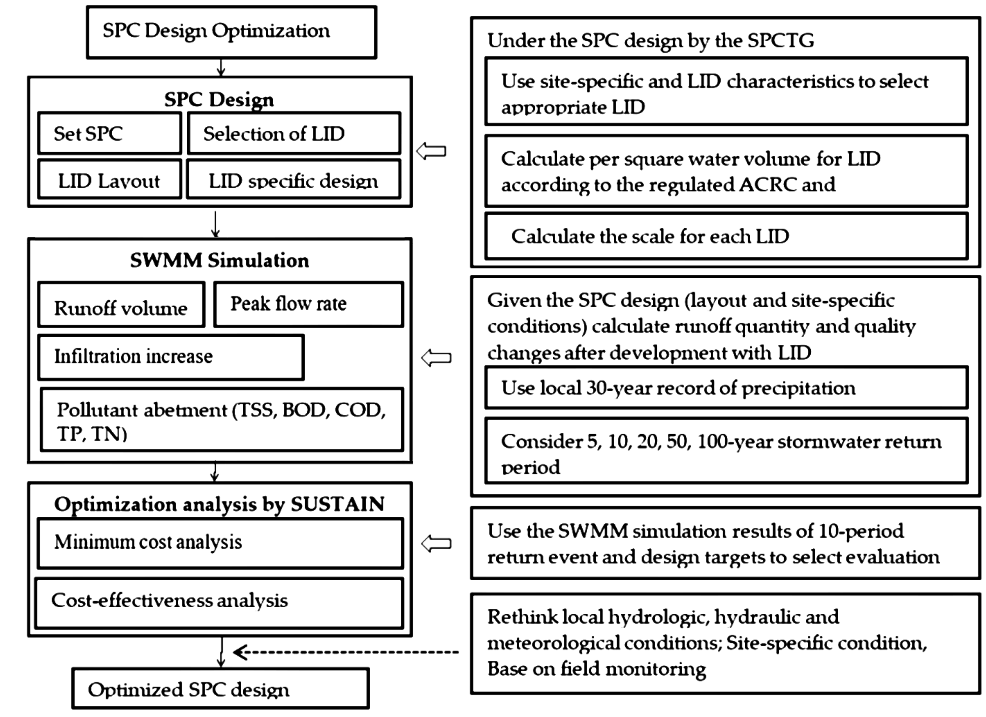
SPC design optimization is an evaluation of all potential SPC design options that meet the ACRC requirement set by the SPCTG to determine the combination of options that minimize total project costs and that is the most cost-effective. The SPC design options include the effects and costs of the LID methods contained within the plan. The optimization process includes three main steps: (1) The design of a SPC under the SPCTG mentioned above, (2) the simulation and calculation of the changes in runoff quantity and quality using SWMM, also, the data from field monitoring of water quality during 3 March to 7 December 2017, was used to calibrate the SWMM model, and (3) the simulation of the minimum cost and the cost-effectiveness of the plan using SUSTAIN. A flowchart of the SPC design optimization method is shown in Figure 1.
2.1. SPC Design
SPC design is based on data related to site-specific soil, hydrological, and hydraulic conditions, as well as local meteorological conditions, particularly rainfall. Based on the SPC SPCTG, the design goals include a reduction in runoff volume and the peak flow rate, and an increase in infiltration as well as pollutant abatement. Pollutants may be represented by a host of parameters, including total suspended solids (TSS), chemical oxygen demand (COD), biological oxygen demand (BOD), total phosphorous (TP), and total nitrogen (TN). As mentioned above, a reduction in runoff volume is often the main goal of SPC design. The only quantitative parameter specified by the SPCTG is the ACRC; the other requirements specified were qualitative. Nonetheless, it is important to control peak flow, pollutant dispersal, and infiltration within SPC designs. Thus, the design objectives should clearly involve these concerns. In addition, the priority of the design goals needs to be determined based on site-specific conditions and used to select appropriate LIDs, as well as suitable evaluation factors for the cost-effectiveness analysis.
According to the different LID characteristics and design goals, various LID options can be selected at the preliminary stage of the design process to meet the ACRC requirement. The ACRC value and the corresponding amount of rainfall needed to determine the reduction in runoff volume per square (m3 m−2), can be obtained from SPCTG documents. The corresponding runoff volume can then be calculated and will be subdivided for each proposed LID by the LID’s area of coverage as shown on the design layout. According to the amount of runoff that each LID will acquire, and the runoff coefficient of each LID, the area of each LID needed to meet ACRC requirement can be calculated and used to calibrate/adjust the area of each LID in the design. However, the design typically needs to be adjusted several times to obtain a final result. A detailed description of the calculation is provided in the SPCTG [3].
This study examined three schemes with different combinations of LID methods that met the SPCTG requirement (ACRC ≤ 0.2). The dimensions and ratios of the LID methods used are listed in Table 1.
2.2. SWMM Simulation
The Stormwater Management Model (SWMM) is widely used by the USA Environmental Protection Agency [8] and is frequently used to model the effects of LID [9,10]. It is especially useful in predicting how the system performs in reducing flood flows [11]. Temporally, it can be used for both the long-term simulation of runoff quantity and quality, or for short-term predictions (e.g., a single event). It is most suitable for modeling the hydrological/stormwater implications of LID in small areas and/or catchments [12].
During the present study, a local 10-year (2005–2015) precipitation and evaporation record was obtained from statistical reports (Table 2 and Table 3), based on the tables, the design precipitation under design control targets can be acquired, then the corresponding 24-h time series could be acquired, which will be used as input for SWMM. The control targets are used conjunction with the designs mentioned previously to assess the reduction in runoff volume and peak flow rate, and to determine increases in infiltration and pollutant (TSS, COD, BOD, TP, TN) abatement. The analysis was conducted for 5 different stormwater return periods: 5, 10, 20, 50, and 100-year events. Three different LID schemes were simulated. The results of the modeling analysis are compared to SPCTG, and discussed for each of the five different return periods. The simulations show differences in the efficiency of the various combinations of LID methods on runoff quantity or quality, rather than simply specifying if they meet the ACRC requirement established by the SPCTG. The estimated result of the average flow reduction for the 10-year event was then used as the input to SUSTAIN optimization module as an evaluation factor (Table 4), the reasons will be discussed following section.
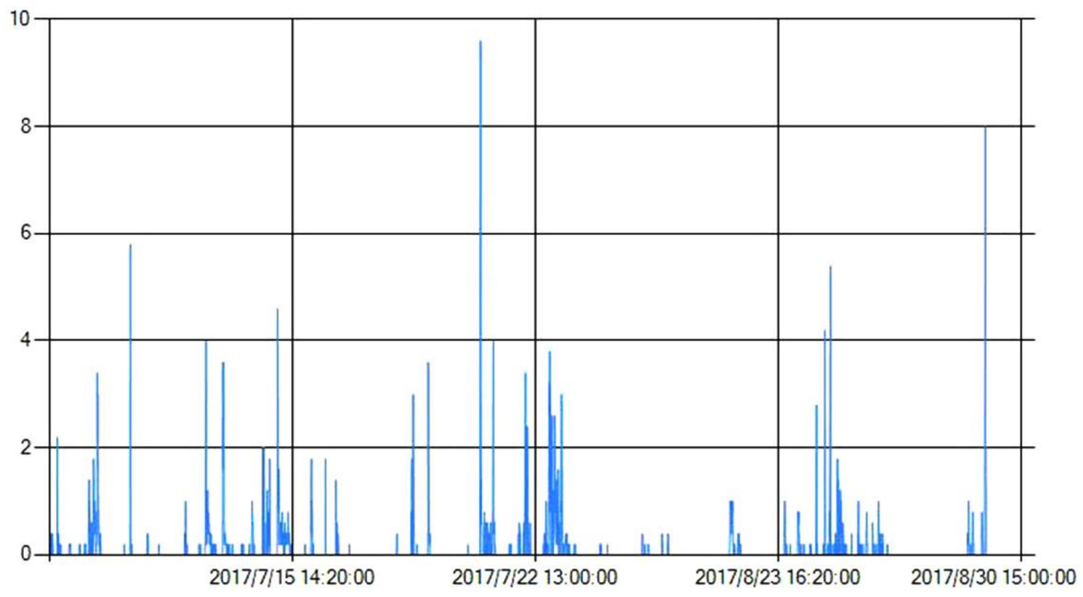
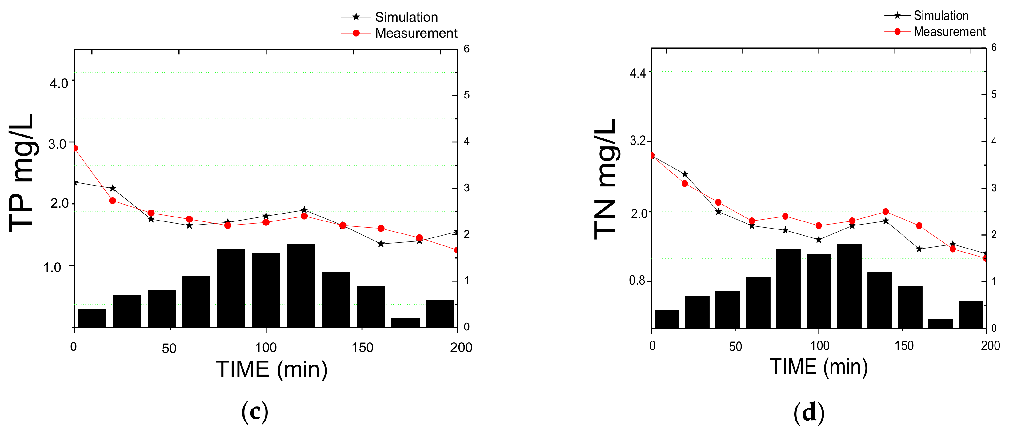
Runoff water quality monitoring data collected during individual flood events at the test site between 3 March and 7 December 2017, and 15 July and 30 August 2017, were used to calibrate the water quality parameters in the SWMM model (Figure 2). The exponential function model inherent in SWMM can most effectively estimate the accumulation and erosion of surface pollutants (TSS, COD, TP, and TN). Thus, it was used in both the pollutant accumulation model and the scour model [13]. The timing between individual runoff events was set at 7 days. The parameters used in the model are listed in Table 5 and shown in Figure 2.
2.3. SUSTAIN Simulation
The System for Urban Stormwater Treatment and Analysis Integration (SUSTAIN) is a decision-support system developed by the USEPA. SUSTAIN can be used to analyze stormwater flow, pollutant discharge, and management options on multiple scales, temporally ranging from a single storm event to long-term, multi-year simulations [13]. By using SUSTAIN, BMP options can be selected and evaluated based on the BMP’s cost and cost-effectiveness. The SUSTAIN modeling approach includes seven key components that are integrated into an ArcGIS platform. It includes a framework manager, ArcGIS interface, watershed model, BMP model, optimization model, post-processor, and Microsoft Access database. The key components are described below [14,15]:
Framework manager: This is the command center of SUSTAIN, built using the ArcGIS platform. It integrates components from the GIS network such as streams and land use with relative simulation modules; it also checks the necessary data for the need for the simulation and optimization components, and plots time series data such as rainfall, runoff, etc.
Watershed module: It integrates local data with watershed simulation models to produce flow and pollutant loading data for the BMP/LID input.
BMP module: It is a simulation-based module to deduce the performance of BMPs.
Optimization module: This module estimates cost, and compares performances and cost for various BMP/LDI options. While meeting user-defined decision criteria, it analyzes combinations of BMPs using two types of optimization search algorithms: Scatter Search and Non-Dominated Sorting Genetic Algorithm-II (NSGA-II). Scatter Search emphasizes relevant outcomes, keeping the ability to produce diverse solutions. It is effective at identifying the near-optimal solution with a specific target value. The Genetic Algorithm focuses on choosing “parents” randomly to produce “offspring” and to randomly select which components of the parents should be combined. NSGA-II is one of most efficient, multi-objective evolutionary algorithms. It performs better in solving the optimization problems related to watershed management than other evolutionary algorithms [15].
SUSTAIN provides two optimization options: Cost minimization and cost-effectiveness. The cost minimization option identifies near-optimal solutions meeting user-specified management targets such as the desired water quality or/and quantity objectives. Cost-effectiveness identifies all cost-effectiveness options within the user-defined management range by developing a BMP/LID cost versus flow or pollutant-reduction effectiveness relationship as illustrated by a cost-effectiveness curve. The optimization equation can be formatted as below.
The objective is to:
For cost minimization, subject to: and/or , where the ith BMP/LID associated with location i, which forms the decision matrix; represent the computed number of water quantity factors, and the maximum (max) value of the water quantity factor targeted at the assessment point j; represent the computed number of water quality loading factors, and the maximum (max) value of the water quality loading targeted at the assessment point k.
For cost-effectiveness, subject to: which represents the range of the flow volume-based stormwater management target; and/or , which represents the range of the pollutant load-based stormwater management target.
To help define the nature of the optimization problem, SUSTAIN was provided with the evaluation factors listed below:
Factors Based on Flow: Peak discharge, annual average flow volume, the frequency of flow exceedance;
Factors Based on Pollutants (TSS, TN, TP, or User Defined): Annual average load, annual average concentration, maximum days for average concentration;
Factors Based on Sediments: Annual average load, annual average concentration, maximum days for average concentration.
During the present study, SUSTAIN was used to simulate the minimum cost and cost-effectiveness of optimal combinations of LIDs. The annual average flow volume was selected as an evaluation factor. The factor (target) was derived from the SWMM simulation and equated for S1 to a 37.78% reduction in flows for events with a 10-year period return. The unit parameter (i.e., width, length, and cost) and unit variables (i.e., threshold, maximum, and increment) were used as typical variables and constraints (Table 5), which were in accordance with SPC design under SPCTG (Table 1).
3. Description of Site
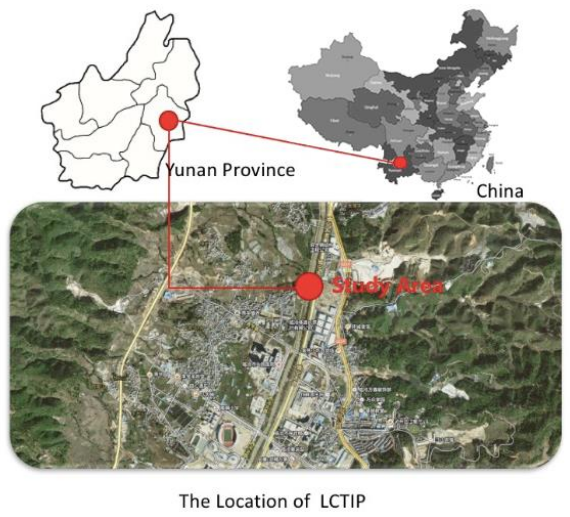
The Lincang Technology Innovation Park (LCTIP) is located in the Lincang City industrial park, Yunnan Province, China (Figure 3), and is the first SPC in Lincang City. The climate is subtropical with an annual rainfall of 1093 mm and an average temperature of 17 °C; relative humidity is 71%.
The land-use is classified as M1, the 1st category of industrial land requiring less adverse environmental impacts than in residential and public areas [16]. The site encompasses an area of 3.78 ha. The terrain slopes at approximately 4.5% from the east (maximum elevation of 1453.2 m) to the west (minimum elevation of 1449.9 m). The land is occupied by buildings, roads, and green space, which is designed as a mixture of commercial, residential, and public facilities. The total construction area is 78,500 m2. The soil is clay. The groundwater is located approximately 1.0–6.8 m below the ground surface.
This project was designed in March 2016 by WALD, and construction was completed at the end of July 2016, when the project was approved by the local authority as a SPC demonstration project. The design objectives for the LCTIP are to (1) reduce the annual runoff volume by 80% (ACRC = 0.2), and (2) remove 60% of the total suspended solids (TSS) as specified by the SPCTG. The investment was $394,000 (all costs presented in US dollars).
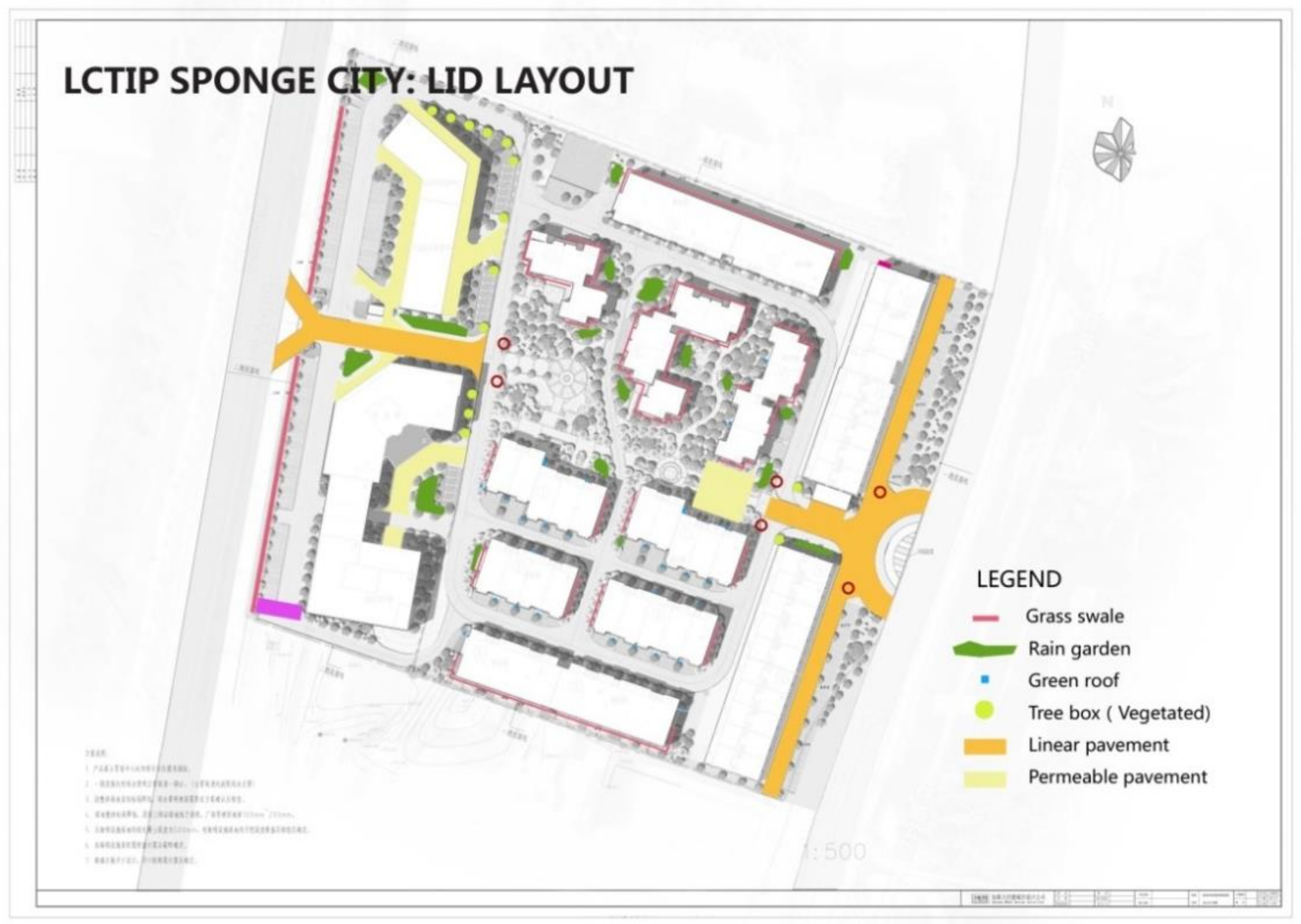
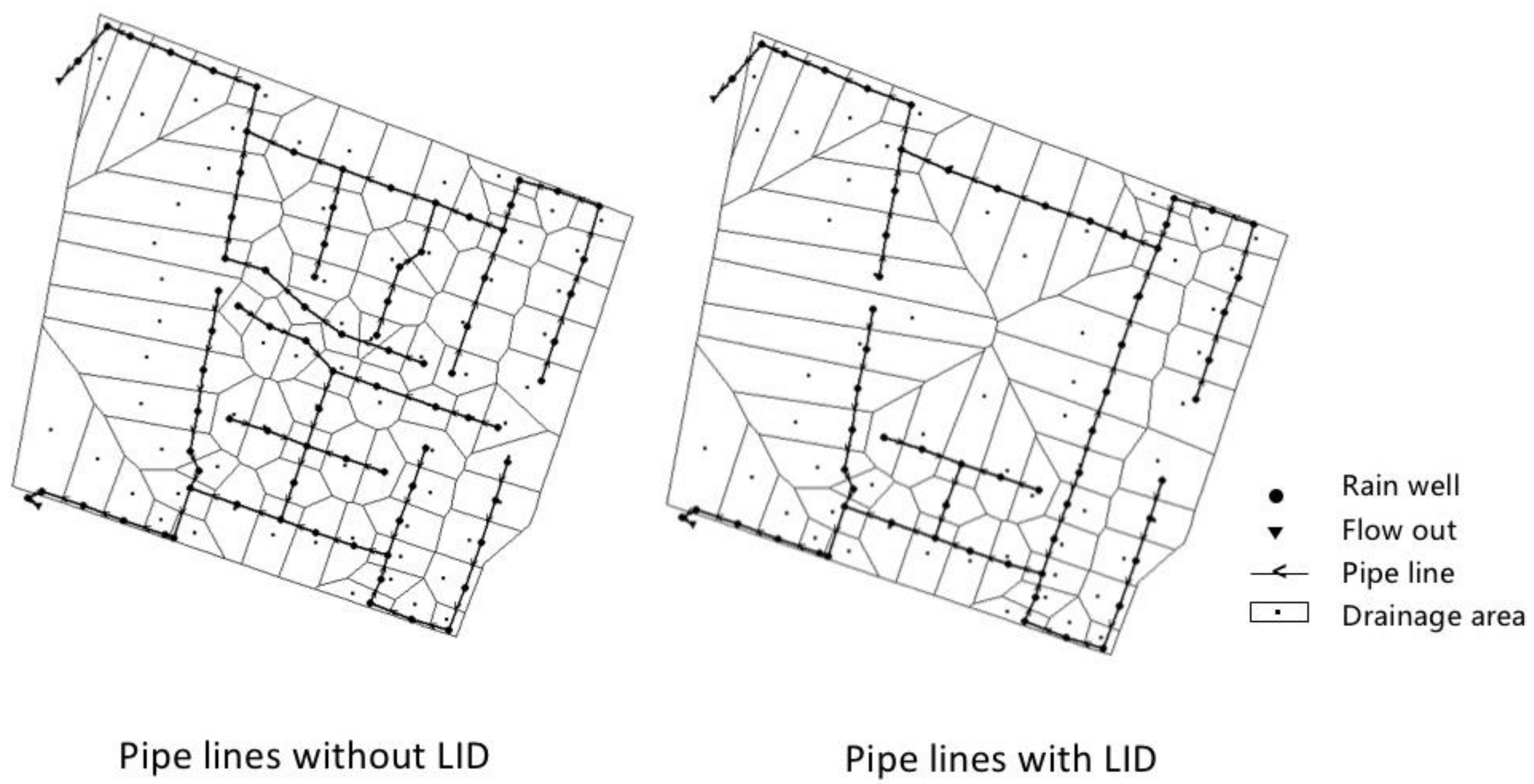
Figure 4 shows the arrangement of the LID measures, including green roofs, grass swales, rain gardens, vegetated areas, permeable pavements, and linear pavements. The total area covered by LIDs is 8382 m2, which is 22% of the total site (3.78 ha). The scale and rationale for each LID are provided in Table 1 as Scheme 1. Figure 5 shows the drainage pipes system.
4. Scenario Analyses and Results
4.1. Scenarios Analyzed under the SPCTG
According to the SPCTG, the LCTIP (located in district II) should exhibit an ACRC of 0.15–0.2 for a corresponding annual rainfall between 22–26.8 mm [3]. Three schemes were designed as follows, each of which met the above ACRC requirement:
- (1)
- Scheme 1 (S1): This is the original plan designed in March 2016, and completed at the end of July 2016. On 28 October 2016, local rainfall reached 75 mm, but there was no accumulation of water on permeable pavement areas. Thus, it has been confirmed by the developer as a reasonable option.
- (2)
- Scheme 2 (S2): This plan was put forth as a landscape improvement design that prioritizes aesthetic amenities, even if those amenities cost more money to build.
- (3)
- Scheme 3 (S3): This plan is the most economical design. This option is intended to meet SPCTG requirements at a minimal cost.
Schemes 2 and 3 are extreme (end-member) options that emphasize either aesthetics or economics, respectively while meeting the ACRC requirements. The various types of LIDs used in both designs are a list in Table 1. S1 has more permeable pavement, S2 has more green land (green spaces), green roofs, and rain gardens, and S3 has more green land.
4.2. Scenario Simulation Results by SWMM
The three schemes were simulated by SWMM to calculate the quantity and quality of changes in runoff. Local 10-year (2005–2015) precipitation and evaporation data were used in the analysis (Table 2 and Table 3) Results of the analyses follow.
4.2.1. SWMM Calibration
The runoff quality was conducted after completion of LCTIP in July 2016. There are 2 rainwater collection points, a rain gauge set on the rooftop of a building, and one rain barrel set onsite. In addition, 3 runoff collection outlets were established on the site, which allowed for the sampling of runoff waters and the determination of pollutant concentrations and loads. Based on water quality analyses conducted between 3 March to 7 December 2017, the mean pollutant loading from runoff is 3.07 mg L−1 for TSS, 21.09 mg L−1 for COD, 0.93 mg L−1 for TP, and 3.88 mg L−1 for TN. These data were used as input for the SWMM simulation. Two independent rainfall events occurring at 14:20 on 15 July 2017, and at 16:20 on 23 August 2017, were used for model calibration of water quality (Figure 2). The outlet water quality monitoring results are shown in Figure 6.
4.2.2. Stormwater Runoff Quantity
Changes in the quantity of runoff (volume reduction, reduction in average flow and peak flow, an increase in infiltration) are shown in Table 4. Changes in runoff quality (TSS, COD, BOD, TP, TN) are shown in Table 7. For S1, runoff volume was reduced from 39.92% to 30.32% when the return period ranged from the 5-year to the 100-year event. The runoff volume changed from 26.4% to 28.57% for S2, and from 10.92% to 8% for S3. S1 was more effective at reducing the volume of runoff than S2 and S3. For all three scenarios, the changes in runoff volume decreased with an increase in the return period.
The amount of infiltration increased from 5.32% to 5.59% for S1 when the return period was between the 5-year to 100-year event. Infiltration increased from 3.29% to 4.66% for S2, and from 6.91% to 5.54% for S3. The change in infiltration as a function of flow recurrence varied between the scenarios. With an increase in the return period, infiltration increased for S2 and decreased for S3. The amount of infiltration did not change as a function of flow frequency for S1.
The average and peak flow magnitude of S1 changed from 38.85% and 21.39% to 24.48% and 28.49%, respectively when the return period changed from the 5-year to 100-year event. For S2, the average and peak flow changed from 28.57% and 41.46% to 27.27% and 41.39%, respectively. For S3, the change was from 14.29% and 52.61% to 11.36% and 51.03%, respectively. These trends indicate that S1 performed better in reducing average flow magnitudes than S2 and S3, but for a reduction in peak flow, S3 was better than S1 and S2. The reduction in average and peak flow magnitudes did not change with an increase in the return period for S2 and S3, but the amount of reduction in both decreased for S1 with an increase in the return period of the event.
In summary, S1 with more permeable pavement performed well with regards to a reduction in runoff volume but performed poorly in reducing peak flow rates. S3, characterized by more green land (green space), performed well with regards to peak flow rate and infiltration, but poorly in reducing runoff volume. S2, characterized by more rain gardens and grass swales, exhibited the least reduction in runoff volume and peak flow rate with an increase in the return period and produced the most increase in infiltration. This is because vegetated LID measures strongly influence infiltration.
4.2.3. Stormwater Runoff Quality
Changes in runoff quality (TSS, COD, BOD, TP, TN) are shown in Table 7. The results indicate that S1 performed better in reducing pollutant loads than S2 and S3. With an increase in the return period from the 5-year to 100-year event, the ability to remove pollutants decreased. For example, decreases in pollutant loads for S1 changed from 62.72% to 53.61% for TSS, from 62.66% to 53.59% for COD, from 62.72% to 53.62% for BOD, from 62.98% to 53.73% for TN, and from 62.97% to 53.75% for TP. The observed decrease was similar for each contaminant and was similar between all three scenarios. For instances, in S2, reductions in loads change from 29.30% to 27.10% for TSS, and from 29.12% to 27.02% for COD, whereas for S3 the reduction changed from 11.17% to 8.01% for TSS, and from 10.84% to 7.8% for COD.
In summary, S1 and S2, which used more LID measures, performed well with regards to the removal of pollutants. In addition, the pollutant removal was similar between the scenarios as return period increased. Some researchers have argued that once TSS pollution is controlled, the other pollutants (COD, BOD, TP, TN) in the SPCTG should also be reduced because these pollutants are strongly associated with fine-grained, chemically reactive solids [17,18].
4.3. Minimum Cost and Cost-Effectiveness Analysis by SUSTAIN
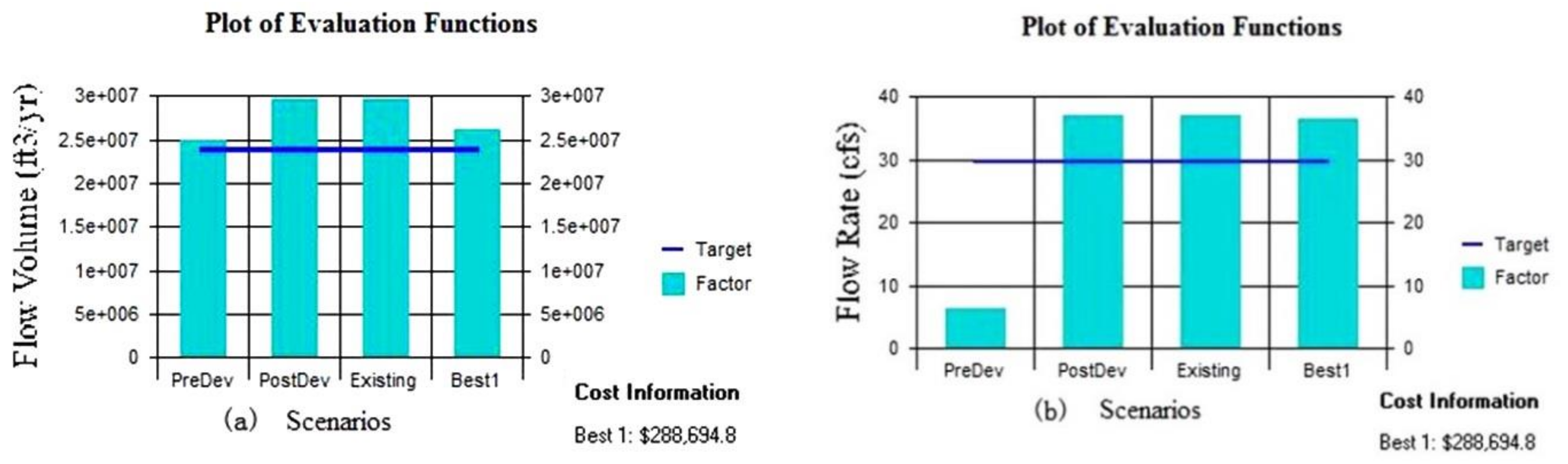
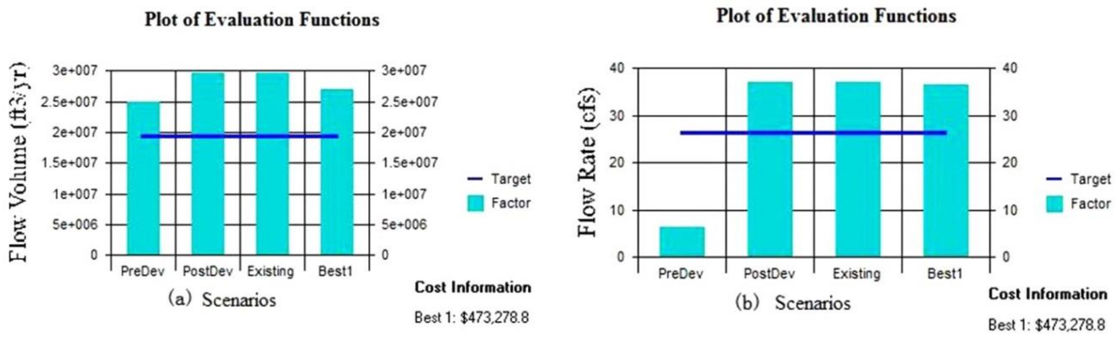
In order to determine the minimum cost and maximum benefit of the SPC design options, the different combinations of LID were assessed. This study selected the annual reduction in flow volume for a 10-year, 24-hour event as an evaluation factor (as described in more detail below). The amount of reduction was based on the results of the SWMM simulation (Table 4a) and equivalent function (1). The control target is a 35% reduction in the annual flow volume for S1, and a 26% reduction for S2, or a 29% reduction in the peak discharge for S1 and a 41% reduction for S2 (Table 4c). The analysis was only conducted on S1 and S2 because S3 only consisted of one type of LID, green land. Thus, no optimization is needed. The characteristics and optimization parameters of the LID used in S1 are shown in Table 6 and Table 8. The result of the minimum cost analysis is $288,695 for S1 and $473,278 for S2 (Figure 8 and Figure 9). As previously mentioned, the investment into (cost of) S1 was $394,000.
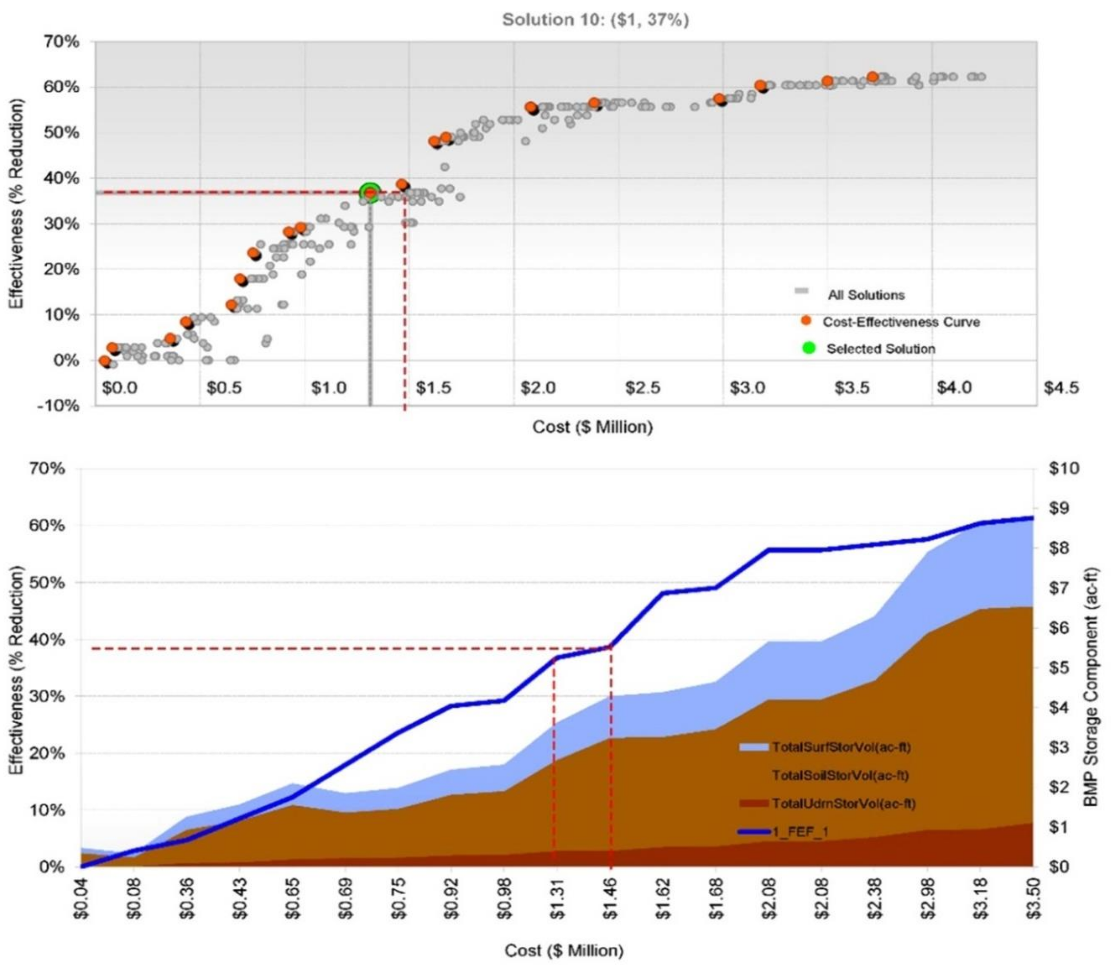
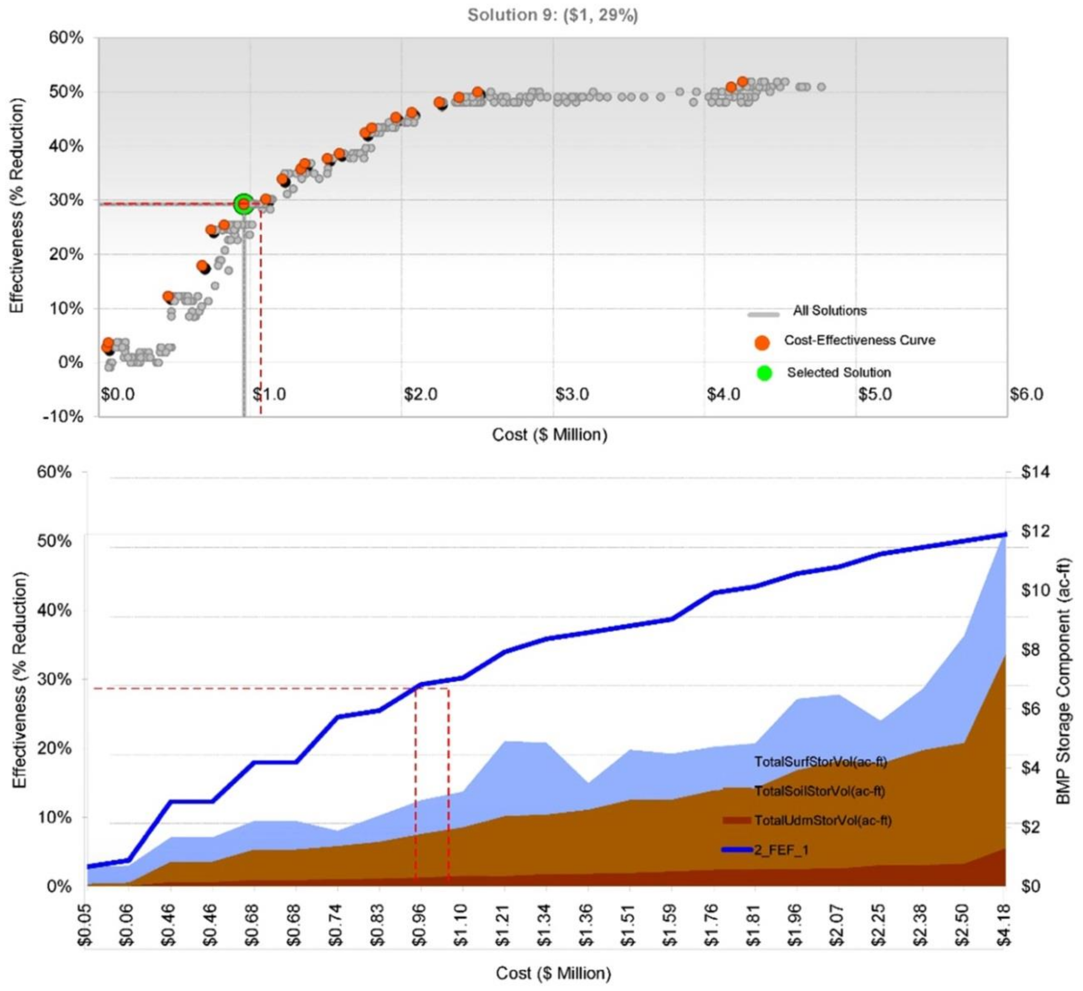
Based on the decision tables, the target value for the cost-effectiveness analysis was assumed to range between 0 and 100 with a 100 m3 s−1 threshold. The search stopping criteria were set as 400 for the maximum number of iterations. The target value range is from 0 to 100%. The cost-effectiveness results for S1 and S2 are shown in Figure 10 and Figure 11. The results indicate that the cost should be $1.37M for S1 when the annual flow volume reduction target was the 37%, and $0.85M for S2 when the annual flow volume reduction target of 28% is met. In addition, the ratio of each LID method used in the various iterative combinations can be acquired (e.g., for S1 in Table 9). The ratio is very helpful because it allows decision-makers to adjust the size of the LIDs used.
5. Discussion
The SPCTG emphasizes small rainfall events. It primarily addresses infiltration and non-point source pollution abatement issues by controlling the runoff volume during precipitation events ranging from 5 to 35 mm [19]. It is less concerned about urban flooding and riverway erosion prevention. However, based on the primary intent of the SPC concept, conservation of the local ecology/ecosystem is very important.
Wang et al. (2015) [19] pointed out that controlling the runoff of a precipitation event with a 10-year return period provides a higher level of runoff control than specified in the SPCTG because it not only addresses infiltration and non-point pollution abatement but preserves the riverway and various types of infrastructure required for the protection of the ecological environment. The reduction of flows for less frequent events will be more difficult to achieve. For example, the required reduction in peak flow discharge for a 10-year event may be only 70–80% of the peak flow reduction needed for an event with a 25-year return period. Specifically, while the 10-year event is significant, achieving the desired results is considered possible. Thus, we selected the 10-year return period for use in the SUSTAIN optimization module.
Based on the SWMM simulation of a 10-year event, the volume reduction was 37.78%, 28.15%, and 10% for S1, S2, and S3, respectively; the peak flow reduction was 28.56%, 41.30%, and 51.98% for S1, S2, and S3, respectively (Table 4). All three schemes, then, meet the SPCGL requirement, especially S1 (the original completed project). However, it still exhibits weakness related to flooding, and ecological preservation, as S3 and S2 performed better at mitigating peak flows and reducing the impacts of flooding. Based on the combination of LID methods for each scheme, the vegetated measures such as rain gardens, bio-retention methods, and green land contribute more to reducing flooding than permeable pavement.
Average changes in water quality after construction compared to before construction were 3.07 mg L−1 to 40 mg L−1 for TSS; 21.09 to 25 mg L−1 for COD; 3.88 to 2.00 mg L−1 for TN, and 0.93 to the 1.0 mg L−1 for TP. With the exception of TP (in which concentrations after and before construction are similar), SI resulted in slightly less COD in the runoff and significantly less TSS in the runoff than observed in the historical data. However, TN concentrations after project construction were almost double. One of the reasons is the fertilizers application to plant. The results indicate that SPC design should be based on site-specific conditions and needs. If the water is relatively clean onsite, then more plants may lead to higher levels of TN.
With regards to the simulations conducted during this study, the calibration of water quality is acceptable (Figure 7). As previously mentioned, the LCTIP is located on the terrain classified as type M1, the 1st industrial land where runoff quality control is a significant issue. Based on the simulation results for a reduction in pollutant loads, S1 and S2 performed better than S3. For example, the reduction in TP during a 10-year event is 60.73% for S1, 28.48% for S2, and 9.63% for S3. The reductions in loads for each of the contaminants examined herein were similar to the trends observed for TP between the three schemes (Table 7). These data indicate that mixing LID methods can perform well with regards to pollutant removal. Moreover, it demonstrates that there is a high degree of correlation between the behavior and removal of many common contaminants (TSS, COD, BOD TN, TP). This conclusion is consistent with the argument in the SPCTG that if TSS is controlled, then other contaminants should also be controlled.
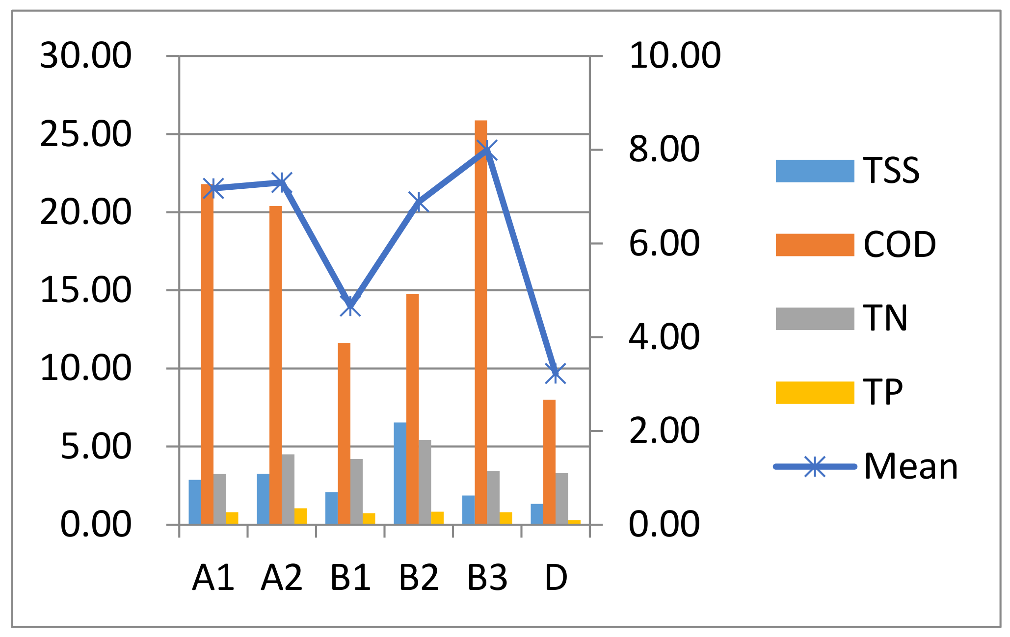
Based on the field monitoring data collected between 3 March and 7 December 2017, four runoff contaminants (TSS, COD, TN, TP) have been significantly mitigated in response to the use of the SPC design shown in Figure 6. In Figure 6, A1 and A2 are inlet points, whereas B1, B2, B3 are outlet points from an area containing dry-land plants, mesic water plants, and fully aquatic (pond) plants. D is the final outlet point where all runoff has flowed through the LID measures. TSS, TN, and TP exhibited lower concentrations than COD. The runoff was light polluted on site. The increase was likely caused by rain gardens and water ponds. After going through the LIDs, the final COD decreased to relatively low levels.
The optimization analysis shows significant differences between the three schemes, although all three designs met the ACRC requirement set in the SPCTG. As previously mentioned, the 10-year event is very significant for the SPC concept; thus, we selected the evaluation factor (a reduction in flow volume), with a 10-year return period for the SPC optimize analysis. The optimization is mainly based on changing various combinations of LID measures toward the control target/evaluation factor; thus S3 was excluded from the optimization analysis.
To compare minimum cost (Figure 8 and Figure 9) to the original cost (Table 1), for S1 the original cost was $329,462, whereas the minimum cost was $288,694, saving 12.3%; but for S2, the original cost was $535,415 while the minimum cost was $473,278, saving 11.6%, respectively.
Based on the cost-effectiveness (Figure 10 and Figure 11), the threshold point for S1 is 58% of volume reduction with a cost of $2.4M. To compare the assumed 10-year event, when runoff reduction is 39% (38% for the 10-year event, Table 4), the cost or potential alternatives is $1.31–$1.46M (the range shown as red square, the optimal point shown as green circle in Figure 10 and Figure 11); it saves 11.5% ($0.15M). The corresponding ratio of the various LIDs is listed in Table 9. The relative percent of the area comprised of rain gardens has increased from 6% to 76%, whereas the relative percent of the area covered in permeable pavement decreased to 8% from 42% in the original alternative by the cost-effectiveness analysis.
Similarly, for S2, the threshold is 50% of volume reduction with a cost of US$2.5M. When the reduction is 29%, the cost is about $0.96–1.1M. At this point, it saves 14.5% ($0.14M). Obviously, the relative percent of the area comprised of rain gardens reached 70%, well above the 1.92% of the original design. The percent covered by green roofs decreased from 13% to 6%, whereas the percent covered by green land declined from 11% to 6%.
The analysis is helpful for decision makers to adjust the type and size of the LIDs used in the design while minimizing project costs. However, the change in the relative use of the various LID methods should be in accordance with project-specific goals. For example, an increase in rain gardens and a decrease in the permeable pavement will likely result in a decrease in the area available for vehicle transportation. Another issue is the need to balance the areas of the landscape that are desirable to build on, with the amount of money needed to build and construct LIDs. The present study proposes a process of optimization for the SPC and provided a potential method to adjust the LIDs used in the design.
Admittedly, the optimization may vary with the use of different evaluation factors and targets. As previously mentioned, several evaluation factors can be selected. It should depend on the SPC design goals. For example, Huang and Zhang (2016) use the removal of 80% of TN and TP as targets to evaluate the SPC [20]. In upstream or public water bodies, the runoff pollutant should be strictly controlled. Moreover, the analysis/design goals should detail what types of constituents need to be controlled (e.g., TSS, TP, TN, COD, BOD), and at what level, rather than rely on an average control level. As previously discussed, S1 can reduce 53% of pollutants on average based on simulation. However, the level of TN removal is 24%, which is lower than the average level.
Normally, according to China meteorological statistics, the annual average precipitation is 660 mm in the north and 1200 mm in the south of China. Northern cities in China exhibit a shortage of water, whereas southern cities exhibit a shortage of good quality water. Therefore, SPC design targets should be distinguished on the basis of local meteorological, hydrologic and geologic factors. Relying on only the ACRC requirement for SPC design is insufficient.
It is very important to conduct field monitoring at constructed sites to accumulate data and develop analytical methods that will help to localize the applications for different cities in China. The application is very similar to the construction of the BMP database in the USA [21]. Therefore, the method of localizing the model is a future research question.
6. Conclusions
China initiated an SPC design and construction method in 2013. Thirty cities in various provinces have been selected as state pilot projects. The SPC design’s main focus is to reach a specified ACRC value regulated by the SPCTG. However, additional controls are needed to improve to the concerns of flood prevention and infrastructure damage inherent in the concept of an SPC. These additional controls need to be aligned with the complex geology and varied meteorology conditions of different areas of China.
This paper presents an approach to optimize SPC design alternatives, in addition to attaining the SPCTG requirement. It fully considers the concerns inherent with an SPC. The method focuses not only on changes in runoff quantity, as described by flow volume, peak flow magnitude (discharge), and infiltration, but also on runoff quality (e.g., expressed by TSS, COD, BOD, TP, and TN). The approach improved the SPC design from focusing on frequent events where infiltration control was the primary concern to events with a longer return period (e.g., the 10-year event) in which flood control was addressed. In addition, based on different evaluation targets and evaluation factors, it can optimize the SPC design through a minimum cost and cost-effectiveness analysis. LCTIP, a SPC project, was chosen as a test scenario. Three schemes that met the SPCTG guidelines were analyzed with 5, 10, 20, 50, and 100-year stormwater return periods.
The three schemes included the original scheme that was actually implemented, a landscape improvement scheme and a minimum cost scheme. The original scheme was completed in July 2016. Water quality runoff from the site was monitoring between March 2017 and December 2017. The results indicate that while all three design options met the ACRC control set in the SPCTG, the designed can be optimized by using selected design targets for cost-effectiveness, which determines the combination of LID measures that require the least financial resources and that produces the greatest benefit. For example, in comparison to the original option, the minimum cost analysis demonstrated that optimal alternative for S1 can save 12.3%, and 15.7% for cost-effectiveness; S2 can save 11.6% for the minimum cost analysis and 4.1% for cost-effectiveness when considering events with a 10-year return period. In addition to these cost-benefit data, the approach provides the corresponding combination LID methods for the SPC, which will help decision makers adjust the SPC design. The approach possesses significant implications to the practical implementation of the SPC program because China is currently investing hundreds of billions of RMB on SPC construction annually.
The collection of site data is very important to the calibration and verification of the SWMM and SUSTAIN models used in the analysis. Thus, it is argued that such data need to be continually collected throughout China.
Author Contributions
Conceptualization, N.L. and C.Q.; Methodology, N.L.; Software, N.L.; Validation, N.L., C.Q. and P.D.; Formal Analysis, N.L.; Investigation, N.L. and C.Q.; Resources, N.L. and C.Q.; Data Curation, N.L.; Writing-Original Draft Preparation, N.L.; Writing-Review & Editing, C.Q.; Visualization, C.Q.; Supervision, P.D.; Project Administration, N.L.; Funding Acquisition, P.D.
Funding
This study was funded by the Major Science and Technology Program for Water Pollution Control and Treatment (Grant number is 2014ZX07323001).
Acknowledgments
The authors thank Lincang Technology Innovation Park and Shenzhen WALD Urban Design Company for providing original designs and data for this study. This research was supported by the Major Science and Technology Program for Water Pollution Control and Treatment No. 2012ZX07302002. The optimization results by SUSTAIN, The Field Monitoring Analysis Report for LCTIP, and The Simulation Results by SWMM for 3 Schemes of LCTIP upon your request.
Conflicts of Interest
The authors declare that they have no conflicts of interest.
References
- Xia, J.; Zhang, Y.Y.; Xiong, L.H.; He, S.; Wang, L.G.; Yu, Z.B. Opportunities and challenges of the sponge city construction related to urban water issues in China. Sci. China Earth Sci. 2017, 60, 652–658. [Google Scholar] [CrossRef]
- Tan, S.K.; Zhang, N. The evaluation of current China sponge city construction—The cases of 16 sponge cites. City Probl. 2016, 6, 98–103. [Google Scholar] [CrossRef]
- Ministry of Housing and Urban-Rural Department (MOHURD). The Guide of Sponge City Construction Technology—LID Technique; Ministry of Housing and Urban-Rural Department: Beijing, China, 2014.
- Che, W.; Zhao, Y.; Li, J.Q.; Wang, W.L.; Wang, J.L.; Wang, S.S.; Gong, Y.W. Explanation of sponge city development technical guide: Basic concepts and comprehensive goals. China Water Wastewater 2015, 31, 1–5. [Google Scholar]
- Ministry of Housing and Urban-Rural Department (MOHURD). Evaluation and Assessment Index of Sponge City Construction Performance (Experiment); Ministry of Housing and Urban-Rural Department: Beijing, China, 2015.
- Ministry of Housing and Urban-Rural Department (MOHURD). Sponge City Specific Plan Design Regulations; Ministry of Housing and Urban-Rural Department: Beijing, China, 2016.
- Xia, J.; Wang, G.S.; Tan, G.; Ye, A.Z.; Huang, G.H. Development of a distributed time-variant gain model for nonlinear hydrological systems. Sci. China Earth Sci. 2005, 34, 1062–1071. [Google Scholar] [CrossRef]
- EPA. Low Impact Development (LID): A Literature Review; The United States Environmental Protection Agency: Washington, DC, USA, 2000.
- Jia, H.F.; Lu, Y.; Yu, S.L.; Chen, Y.R. Planning of LID–BMPs for urban runoff control: The case of Beijing Olympic Village. Sep. Purif. Technol. 2012, 84, 112–119. [Google Scholar] [CrossRef]
- Qi, H.J. Design and Performance Simulation of LID Measures of Rainwater Management. Master’s Thesis, Beijing Architecture University, Beijing, China, 2013. [Google Scholar]
- Xu, P.J. SWMM application in urban anti-flooding. Sichuan Archit. 2015, 35, 271–273. [Google Scholar]
- Elliott, A.H.; Trowsdale, S.A. A review of models for low impact urban stormwater drainage. Environ. Model Softw. 2007, 22, 394–405. [Google Scholar] [CrossRef]
- Wu, J.L. Evaluation and Application of the Typical Method for Urban Water Utilization of Low Impact Development. Master’s Thesis, Harbin Industrial University, Harbin, China, 2012. [Google Scholar]
- Lee, J.H.; Bang, K.W.; Ketchum, L.H.; Choe, J.S.; Yu, M.J. First flush analysis of urban storm runoff. Sci. Total Environ. 2002, 293, 163–175. [Google Scholar] [CrossRef]
- Lai, F.H.; Zhen, J.; Riverson, J.; Shoemaker, J. SUSTAIN—An evaluation and cost-optimization tool for placement of BMPs. In Proceedings of the World Environmental and Water Resources Congress, Omaha, NE, USA, 21–25 May 2006; American Society of Civil Engineers: Reston, VA, USA, 2012. [Google Scholar]
- Ministry of Housing and Urban-Rural Department (MOHURD). City Landuse Classification and Standard (GB50137-20); P.R.C. Housing and Urban Construction Department: Beijing, China, 2012.
- Horowitz, A.J. A Primer on Sediment-Trace Element Chemistry, 2nd ed.; Lewis: Chelsea, UK, 1991. [Google Scholar]
- Miller, J.R. Contaminated Rivers: A Geomorphological-Geochemical Approach to Site Assessment and Remediation; Springer: Dordrecht, The Netherlands, 2007. [Google Scholar]
- Wang, H.; Ding, L.Q.; Li, N. Urban runoff control criteria under sponge city concept. Spec. Top. 2015, 25, 10–15. [Google Scholar] [CrossRef]
- Huang, L.J.; Zhang, P. The indicators weight analysis for sponge city evaluation. J. Green Sci. Technol. 2016, 22, 117–122. [Google Scholar]
- Clary, J.; Urbonas, B.; Jones, J.; Strecker, E.; Quigley, M.; O’Brien, J. Developing, evaluating and maintaining a standardized stormwater BMP effectiveness database. Water Sci. Technol. 2002, 45, 65–73. [Google Scholar] [CrossRef] [PubMed]
Figure 1.
Flow chart showing the proposed sponge city (SPC) design optimization process.

Figure 2.
Time series plot of rainfall recorded by an onsite gauge (mm).

Figure 3.
Map showing the location of the Lincang Technology Innovation Park (LCTIP) test site in Yunan Province, China.
Figure 3.
Map showing the location of the Lincang Technology Innovation Park (LCTIP) test site in Yunan Province, China.

Figure 4.
Spatial distribution of low impact development measures used at the LCTIP test site (S1).

Figure 5.
The pipeline drainage system at the LCTIP with and without low impact development.

Figure 6.
The results of onsite water quality monitoring between 3 March and 7 December 2017.

Figure 7.
Comparison of measured (observed) and simulated concentrations for selected water quality parameters at the LCTIP (Lower filled bars represent the intensity of rainfall); (a) TSS; (b) COD; (c) TP; (d) TN.
Figure 7.
Comparison of measured (observed) and simulated concentrations for selected water quality parameters at the LCTIP (Lower filled bars represent the intensity of rainfall); (a) TSS; (b) COD; (c) TP; (d) TN.


Figure 8.
The minimum cost analysis for S1 (US dollar); (a) Flow Volume; (b) Flow Rate.

Figure 9.
The minimum cost analysis for S2 (US dollar); (a) Flow Volume; (b) Flow Rate

Figure 10.
The cost-effectiveness analysis for S1.

Figure 11.
The cost-effectiveness analysis for S2.


Table 1.
Comparison of the Three Design Schemes for Lincang Technology Innovation Park (LCTIP); the total land area is 3.78 ha.
Table 1.
Comparison of the Three Design Schemes for Lincang Technology Innovation Park (LCTIP); the total land area is 3.78 ha.
| LIDs | Scheme 1 (S1) | Scheme 2 (S2) | Scheme 3 (S3) | |||||||
|---|---|---|---|---|---|---|---|---|---|---|
| Unit Price ($ m−2) | Area (m2) | Ratio (%) | Cost ($) | Area (m2) | Ratio (%) | Cost ($) | Area (m2) | Ratio (%) | Cost ($) | |
| Green Roof | 46 | 1442 | 3.81 | 66,315 | 5013 | 13.2 | 230,590 | |||
| Grass Swale | 92 | 594 | 1.57 | 54,657 | 492 | 1.3 | 45,293 | |||
| Rain Garden | 185 | 500 | 1.32 | 92,426 | 726 | 1.9 | 134,349 | |||
| Vegetated ** | 138 | 30 | 0.08 | 4168 | 132 | 0.3 | 18,183 | |||
| Permeable Pavement | 31 | 3508 | 9.27 | 108,736 | 1443 | 3.8 | 44,745 | |||
| Linear Pavement * | 1.4 | 2259 | 5.97 | 3162 | ||||||
| Green Land | 15.4 | 4043 | 10.6 | 62,255 | 9499 | 25.1 | 146,290 | |||
| Total | 8328 | 22 | 329,462 | 10,578 | 31.3 | 535,415 | 9499 | 25.1 | 146,290 | |
* Linear Drainage Pavement, Runoff coefficient is 0.9; ** Tree box etc. Table Comparison of the Three Design Schemes for LCTIP; the total land area is 3.78 ha.
Table 2.
Historical Precipitation data from Lincang City (2005–2015, mm).
| Year | Jan | Feb | Mar | April | May | June | July | Aug | Sep | Oct | Nov | Dec | Total |
|---|---|---|---|---|---|---|---|---|---|---|---|---|---|
| 2005 | 0.7 | 1.9 | 40.1 | 18.8 | 25.7 | 161.4 | 182.4 | 354.3 | 70.3 | 104.4 | 18.1 | 23.1 | 1001.2 |
| 2006 | 27.9 | 0.9 | 4.4 | 61.5 | 213.6 | 141.5 | 255.1 | 208.4 | 133.3 | 278.9 | 22.7 | 14.5 | 1334.8 |
| 2007 | 6.5 | 52.7 | 0.2 | 34.1 | 188.5 | 133.3 | 349.4 | 230.8 | 179.1 | 138.5 | 9.4 | 1322.5 | |
| 2008 | 22.3 | 6.0 | 14.2 | 13.3 | 91.4 | 195.4 | 186.9 | 217.1 | 97.0 | 100.2 | 59.9 | 12.6 | 1016.3 |
| 2009 | 10.9 | 5.5 | 64.1 | 69.4 | 109.7 | 199.1 | 283.0 | 81.9 | 66.5 | 27.5 | 0.2 | 917.8 | |
| 2010 | 1.9 | 2.8 | 24.8 | 70.5 | 32.8 | 107.2 | 290.6 | 237.1 | 205.8 | 150.2 | 4.6 | 58.8 | 1187.1 |
| 2011 | 28.3 | 0.0 | 31.4 | 57.5 | 107.9 | 133.0 | 227.9 | 193.5 | 211.2 | 61.4 | 33.1 | 8.7 | 1093.9 |
| 2012 | 17.7 | 0.0 | 35.6 | 22.4 | 86.9 | 175.7 | 240.1 | 90.6 | 87.6 | 44.5 | 78.8 | 879.9 | |
| 2013 | 1.9 | 0.9 | 18.0 | 12.7 | 95.6 | 136.5 | 265.0 | 261.0 | 165.3 | 169.9 | 5.5 | 25.9 | 1158.2 |
| 2014 | 0.0 | 13.7 | 6.2 | 10.3 | 31.9 | 160.3 | 295.9 | 141.5 | 158.9 | 37.5 | 23.1 | 9.3 | 888.6 |
| 2015 | 188.7 | 5.3 | 14.6 | 31.3 | 33.9 | 94.1 | 279.9 | 199.3 | 179.4 | 114.9 | 44.1 | 31.6 | 1217.1 |
| Mean | 27.9 | 8.4 | 17.7 | 36.0 | 88.9 | 140.7 | 252.0 | 219.7 | 142.7 | 115.2 | 29.7 | 20.5 | 1092.5 |
Table 3.
Historical Evaporation data from Lincang City (2005–2015) (mm).
| Year | Jan | Feb | Mar | April | May | June | July | Aug | Sep | Oct | Nov | Dec | Total |
|---|---|---|---|---|---|---|---|---|---|---|---|---|---|
| 2005 | 73.2 | 103.8 | 98.4 | 130.3 | 139.5 | 100.1 | 86.8 | 75.8 | 88.4 | 70.7 | 66.8 | 58.5 | 1092.3 |
| 2006 | 75.4 | 82.5 | 128.0 | 119.9 | 80.0 | 86.9 | 84.8 | 111.3 | 86.7 | 74.6 | 73.5 | 64.2 | 1067.8 |
| 2007 | 69.8 | 70.8 | 131.2 | 99.0 | 84.9 | 103.1 | 52.6 | 70.9 | 74.3 | 70.2 | 74.5 | 70.9 | 972.2 |
| 2008 | 78.9 | 87.2 | 94.8 | 124.1 | 107.4 | 74.7 | 81.4 | 83.1 | 89.8 | 70.5 | 76.3 | 60.1 | 1025.6 |
| 2009 | 65.2 | 102.2 | 112.9 | 109.7 | 115.8 | 82.7 | 84.2 | 84.4 | 90.9 | 98.8 | 83.2 | 69.9 | 1099.9 |
| 2010 | 78.3 | 97.2 | 118.9 | 126.2 | 113.1 | 77.5 | 71.4 | 90.0 | 85.7 | 73.7 | 63.6 | 64.3 | 1059.7 |
| 2011 | 63.5 | 87.9 | 102.9 | 105.9 | 99.6 | 77.2 | 86.7 | 92.7 | 83.9 | 77.2 | 66.5 | 63.1 | 1007.1 |
| 2012 | 72.2 | 100.8 | 112.7 | 113.7 | 118.6 | 74.0 | 68.9 | 94.5 | 72.3 | 96.6 | 71.4 | 78.4 | 1074.1 |
| 2013 | 77.6 | 97.8 | 125.2 | 127.9 | 95.9 | 90.2 | 57.2 | 85.6 | 77.7 | 71.1 | 80.7 | 65.0 | 1051.9 |
| 2014 | 74.2 | 85.9 | 118.2 | 131.3 | 127.5 | 91.3 | 75.2 | 64.5 | 76.1 | 73.1 | 79.5 | 69.4 | 1066.2 |
| 2015 | 39.7 | 58.7 | 100.3 | 71.0 | 99.5 | 60.3 | 54.9 | 33.4 | 42.6 | 62.4 | 47.3 | 40.0 | 710.1 |
| Mean | 69.8 | 88.6 | 113.0 | 114.5 | 107.4 | 83.5 | 73.1 | 80.6 | 78.9 | 76.3 | 71.2 | 64.0 | 1020.6 |
Table 4.
Changes (%) in Runoff Quantity for Scenarios 1–3 for selected 24 h recurrence intervals.
| (a) Runoff volume reduction (%) | (b) Increases in Runoff Filtration (%) | ||||||||||
|---|---|---|---|---|---|---|---|---|---|---|---|
| 5 y | 10 y | 20 y | 50 y | 100 y | 5 y | 10 y | 20 y | 50 y | 100 y | ||
| −24 h | −24 h | −24 h | −24 h | −24 h | −24 h | −24 h | −24 h | −24 h | −24 h | ||
| S1 | 39.92 | 37.78 | 35.1 | 32.56 | 30.32 | S1 | 5.59 | 5.33 | 5.11 | 5.28 | 5.32 |
| S2 | 28.57 | 28.15 | 27.57 | 26.82 | 26.4 | S2 | 3.29 | 3.85 | 4.03 | 4.32 | 4.66 |
| S3 | 10.92 | 10 | 9.3 | 8.45 | 8 | S3 | 6.91 | 6.51 | 6.45 | 5.76 | 5.54 |
| (c) Average flow (%) | (d) Peak flow reduction (%) | ||||||||||
| 5 y | 10y | 20 y | 50 y | 100 y | 5 y | 10 y | 20 y | 50 y | 100 y | ||
| −24 h | −24 h | −24 h | −24 h | −24 h | −24 h | −24 h | −24 h | −24 h | −24 h | ||
| S1 | 38.85 | 35.38 | 31.51 | 27.67 | 24.48 | S1 | 21.39 | 28.56 | 28.55 | 28/89 | 28.49 |
| S2 | 28.57 | 25.81 | 28.57 | 27.5 | 27.27 | S2 | 41.46 | 41.3 | 41.33 | 41.36 | 41.39 |
| S3 | 14.29 | 9.68 | 11.43 | 10 | 11.36 | S3 | 52.61 | 51.98 | 51.53 | 51.16 | 51.03 |
Table 5.
Characteristics of low-impact development (LID) methods used to SUSTAIN for S1.
| LIDs | Size | Soil Parameters | |||||
|---|---|---|---|---|---|---|---|
| Width (m) | Area (m2) | Slope (%) | Thickness (mm) | Porosity | Water Capacity | Withering Point | |
| Green Roof | 12 | 1442 | — | 500 | 0.463 | 0.232 | 0.116 |
| Grass Swale | 3 | 594.1 | 50 | 500 | 0.5 | 0.105 | 0.047 |
| Rain Garden | 20 | 499.6 | — | 300 | 0.463 | 0.232 | 0.116 |
| Vegetated | 18 | 30.2 | — | 300 | 0.5 | 0.105 | 0.047 |
| Permeable Pavement | 8 | 5766.5 | — | 60 | 0.21 | — | — |
Table 6.
Accumulation and flush function parameter values used in the analysis.
| Type | Pollutants | Max. Buildup (kg ha−1) | Rate | Wash off Coefficient | Wash off Exponent | Cleaning Efficient | BMP Efficient |
|---|---|---|---|---|---|---|---|
| Roof | TSS | 21 | 0.5 | 0.007 | 1.7 | 0 | 0 |
| COD | 25 | 0.4 | 0.001 | 0.6 | 0 | 0 | |
| TP | 2 | 0.004 | 1.3 | 0 | 0 | ||
| TN | 4 | 0.003 | 1.6 | 0 | 0 | ||
| Road | TSS | 25 | 0.5 | 0.005 | 1.4 | 70 | 0 |
| COD | 13 | 0.4 | 0.006 | 0.4 | 70 | 0 | |
| TP | 2 | 0.002 | 1.4 | 70 | 0 | ||
| TN | 4 | 0.001 | 1.3 | 70 | 0 | ||
| Grass | TSS | 12 | 0.5 | 0.008 | 1.6 | 0 | 50 |
| COD | 8 | 0.4 | 0.003 | 0.4 | 0 | 50 | |
| TP | 4 | 0.002 | 1.8 | 0 | 50 | ||
| TN | 6 | 0.003 | 1.5 | 0 | 50 |
Table 7.
Pollutants reduction (%) for Schemes 1–3 for selected 24 h recurrence intervals.
| TSS | COD | ||||||||||
|---|---|---|---|---|---|---|---|---|---|---|---|
| 5 y | 10 y | 20 y | 50 y | 100 y | 5 y | 10 y | 20 y | 50 y | 100 y | ||
| −24 h | −24 h | −24 h | −24 h | −24 h | −24 h | −24 h | −24 h | −24 h | −24 h | ||
| S1 | 62.72 | 60.52 | 58.26 | 55.7 | 53.61 | S1 | 62.66 | 60.48 | 58.23 | 55.67 | 53.59 |
| S2 | 29.3 | 28.81 | 28.4 | 27.7 | 27.1 | S2 | 29.12 | 28.66 | 28.28 | 27.59 | 27.02 |
| S3 | 11.37 | 10.35 | 9.52 | 8.6 | 8.01 | S3 | 10.84 | 9.94 | 9.19 | 8.34 | 7.8 |
| BOD | TN | ||||||||||
| 5 y | 10y | 20 y | 50 y | 100 y | 5 y | 10 y | 20 y | 50 y | 100 y | ||
| −24 h | −24 h | −24 h | −24 h | −24 h | −24 h | −24 h | −24 h | −24 h | −24 h | ||
| S1 | 62.72 | 60.52 | 58.26 | 55.7 | 53.62 | S1 | 62.98 | 60.74 | 58.44 | 55.84 | 53.73 |
| S2 | 29.11 | 28.66 | 28.29 | 27.59 | 27.97 | S2 | 28.99 | 28.56 | 28.21 | 27.52 | 26.96 |
| S3 | 10.78 | 9.9 | 9.16 | 8.32 | 8.98 | S3 | 10.56 | 9.73 | 9.03 | 8.21 | 7.69 |
| TP | |||||||||||
| 5 y | 10 y | 20 y | 50 y | 100 y | |||||||
| −24 h | −24 h | −24 h | −24 h | −24 h | |||||||
| S1 | 62.97 | 60.73 | 58.43 | 55.85 | 53.75 | ||||||
| S2 | 28.89 | 28.48 | 28.15 | 27.47 | 26.81 | ||||||
| S3 | 10.41 | 9.63 | 8.97 | 8.14 | 7.64 | ||||||
Table 8.
Optimization parameters of LID used for S1.
| LIDs | Unit Parameters | Unit Variables | ||||
|---|---|---|---|---|---|---|
| Width (m) | Length (m) | Price ($ m−2) | Threshold | Maximum | Increment | |
| Green Roof | 12 | 12 | 46 | 10 | 25 | 5 |
| Grass Swale | 3 | 20 | 92 | 10 | 80 | 10 |
| Rain Garden | 20 | 25 | 185 | 5 | 25 | 5 |
| Vegetated | 18 | 20 | 138 | 20 | 50 | 10 |
| Permeable Pavement | 8 | 15 | 31 | 25 | 50 | 5 |
Table 9.
The ratios of each LID for the optimal alternative of S1.
| LIDs | S1 | S2 | ||
|---|---|---|---|---|
| Ratio | Cost ($ M) | Ration | Cost ($ M) | |
| Green Roof | 8% | 0.118 | 6% | 0.058 |
| Grass Swale | 3% | 0.044 | 5% | 0.048 |
| Rain Garden (Bio-Retention) | 76% | 1.117 | 70% | 0.672 |
| Vegetated (Infiltration Trench) | 3% | 0.044 | 5% | 0.048 |
| Permeable Pavement | 10% | 0.147 | 8% | 0.077 |
| Green Land | 6% | 0.058 | ||
© 2018 by the authors. Licensee MDPI, Basel, Switzerland. This article is an open access article distributed under the terms and conditions of the Creative Commons Attribution (CC BY) license (http://creativecommons.org/licenses/by/4.0/).
Share and Cite
MDPI and ACS Style
Li, N.; Qin, C.; Du, P. Optimization of China Sponge City Design: The Case of Lincang Technology Innovation Park. Water 2018, 10, 1189. https://doi.org/10.3390/w10091189
AMA Style
Li N, Qin C, Du P. Optimization of China Sponge City Design: The Case of Lincang Technology Innovation Park. Water. 2018; 10(9):1189. https://doi.org/10.3390/w10091189
Chicago/Turabian StyleLi, Nan, Chengxin Qin, and Pengfei Du. 2018. "Optimization of China Sponge City Design: The Case of Lincang Technology Innovation Park" Water 10, no. 9: 1189. https://doi.org/10.3390/w10091189
Note that from the first issue of 2016, this journal uses article numbers instead of page numbers. See further details here.