Article

A Copula-Based Bayesian Network for Modeling Compound Flood Hazard from Riverine and Coastal Interactions at the Catchment Scale: An Application to the Houston Ship Channel, Texas

by
Anaïs Couasnon
1,2,*,
Antonia Sebastian
2 and
Oswaldo Morales-Nápoles
2
1
Institute for Environmental Studies, Faculty of Science, Vrije Universiteit Amsterdam, De Boelelaan 1087, 1081 HV Amsterdam, The Netherlands
2
Faculty of Civil Engineering and Geosciences, Delft University of Technology, Stevinweg 1, 2628 CN Delft, The Netherlands
*
Author to whom correspondence should be addressed.
Water 2018, 10(9), 1190; https://doi.org/10.3390/w10091190
Submission received: 3 August 2018 / Revised: 28 August 2018 / Accepted: 30 August 2018 / Published: 4 September 2018

Abstract

:
Traditional flood hazard analyses often rely on univariate probability distributions; however, in many coastal catchments, flooding is the result of complex hydrodynamic interactions between multiple drivers. For example, synoptic meteorological conditions can produce considerable rainfall-runoff, while also generating wind-driven elevated sea-levels. When these drivers interact in space and time, they can exacerbate flood impacts, a phenomenon known as compound flooding. In this paper, we build a Bayesian Network based on Gaussian copulas to generate the equivalent of 500 years of daily stochastic boundary conditions for a coastal watershed in Southeast Texas. In doing so, we overcome many of the limitations of conventional univariate approaches and are able to probabilistically represent compound floods caused by riverine and coastal interactions. We model the resulting water levels using a one-dimensional (1D) steady-state hydraulic model and find that flood stages in the catchment are strongly affected by backwater effects from tributary inflows and downstream water levels. By comparing our results against a bathtub modeling approach, we show that simplifying the multivariate dependence between flood drivers can lead to an underestimation of flood impacts, highlighting that accounting for multivariate dependence is critical for the accurate representation of flood risk in coastal catchments prone to compound events.

1. Introduction

Coastal cities suffer from extreme flood risks, being both exposed to multiple hazard types and gathering high asset values and critical infrastructure [1]. They experience different sources of flooding driven by the interaction of oceanographic, hydrological, geological, and meteorological processes [2]. It was estimated that in 2000, about 10% of the global population (625 million people) lived in the area below 10 m of elevation with a direct connection to the sea [3]. More specifically, port cities fostering rapid socio-economic development are flood risk hotspots. Hallegatte et al. [4] estimated more than an eight-fold increase in global economic average annual flood losses for major coastal port cities (from US$6 billion in 2005 to US$52 billion by 2050) due to socio-economic changes alone suggesting that the risk of compound flooding, especially in those areas, will grow over time. Thus, detailed flood probability estimates are critically needed for future coastal resilience.
Modeling flood hazards in coastal catchments is a complex undertaking. Synoptic meteorological conditions can generate both considerable rainfall and anomalously high coastal water levels. For example, Atlantic cyclones have been well documented as causing high surge levels and heavy precipitation [5,6,7,8,9,10]. The importance of this interaction in determining the flood level and magnitude in coastal catchments is dependent on the storm and the catchment properties [11]. Large catchments typically exhibit a lag of several days between high sea levels and high river levels such that the flood events may not physically interact depending on their magnitude and duration. For example, the Rhine delta experiences on average a lag of about six days between high sea levels at the coast and high-water level at Lobith in the Netherlands [12]. In contrast, smaller catchments often have riverine flood wave travel times of less than a day [13]. If co-occurring with a coastal storm surge event, the high river discharges are obstructed by the anomalously high sea-level which may exacerbate the flood stage in the coastal catchment. The joint occurrence of both riverine and coastal floods leading to an extreme impact, here the flood level, is referred to as compound flooding [14,15,16].
Despite increasing scientific recognition of compound flooding [14], regulatory flood hazard maps seldom systematically include the impacts of riverine and coastal interactions [17]. One typical approach used in the US is to consider these two processes separately and merge the independently obtained coastal and riverine flood hazard maps by combining the respective rate of occurrence of a given modeled water surface elevation [17,18]. In doing so, the dependence between these two flood processes is neglected, providing a simplified representation of the flood extent and thereby the flood hazard characterization. Continental to global scale coastal or riverine studies often model flooding due to one flood driver only [19,20,21,22,23,24]. River discharge and storm surge interactions are highly dependent on the geometry of the cross-sections and the slope of the river bed, generating nonlinear responses in the flood extent and amplitude along the river [25]. Several local studies have highlighted the importance of modeling compound flooding to better characterize flood hazard in coastal catchments [26,27,28,29]. For example, Kumbier et al. [27] found that neglecting river discharge when modeling the June 2016 storm event in the Shoalhaven Estuary (Australia) underestimated the flood extent by 30%. As they only focus on one event, these modeling scenarios do not allow further analysis on the impact of compound flood for flood hazard analysis.
To better capture the behavior of compound events, previous researchers have focused on the statistical dependence between river and coastal floods since it is inherently linked with the joint probability analysis [30,31,32]. The strength of the statistical dependence between flood hazards is usually quantified by means of proxy variables [16,33]. Zheng et al. [34] pointed out that even a weak dependence between flood drivers can have significant implications for estimating the flood hazard. Ward et al. [35] used non-parametric correlation coefficients and copula structures to quantify the statistical dependence between coastal and river floods. Salvadori et al. [36] developed a theoretical framework to quantify multivariate return periods from copulas according to predefined hazard scenarios (for a developed and extensive summary, see also Reference [37]). This framework was also applied by Moftakhari et al. [38] to characterize compound flooding caused by the interactions between river flows and sea-level rise. However, while these probability and dependence assessments of compound extremes are valuable, they do not provide direct guidance on the expected impacts within the catchment. Moreover, flood drivers of different levels which are not themselves extreme may combine to create an extreme impact [14,39].
To model compound flood events at the catchment scale, multiple boundary conditions are needed such that a univariate or bivariate analysis alone may not be sufficient to characterize the flood hazard. A traditional univariate method consists of compartmenting the river network into single river reaches and modeling flood extent and/or depth at the latter spatial extent [40]. This becomes problematic when integrating results at the catchment scale since river reaches are physically connected [41,42]. The discharge downstream of a confluence results from the contribution of its upstream tributaries. A given downstream river discharge may be obtained by a large combination of upstream river flows which, when modeled, can result in different flood extents. The spatial dependence of discharge between tributaries clearly becomes important to identify possible combinations. Consequently, in order to derive the flood extent and its associated annual exceedance probability, a realistic spatial dependence structure between tributaries is needed [40,43].
Few studies have quantified the flood hazard while also including multiple flood drivers. Those that have, analyzed results at point locations within the catchment rather than showing results for the whole river segment. For example, Lamb et al. [44] represented the joint multivariate distribution with a multivariate statistical model based on conditional exceedance. Once the statistical model was built, they were able to simulate large series of synthetic events and compute the damage at selected locations, using discharge–damage curves. Bevacqua et al. [28] used pair–copula constructions and a multiple regression model to predict the water level at one selected location along a coastal river reach. Their results showed that neglecting the dependence between discharge and sea-level underestimated the flood hazard at that location. However, to the best of our knowledge, this has not been studied for the whole river section in a probabilistic manner.
This paper introduces an alternative method to model and assesses the impact of compound flooding from riverine and coastal interactions at the catchment scale while accounting for spatial dependence between river tributaries. A Bayesian Network (BN) is constructed and used to simulate a set of synthetic joint boundary conditions needed to model water levels in a coastal catchment vulnerable to compound flooding. Unlike conventional univariate models, this model integrates the spatial dependence between river tributaries as well as the dependence between river and coastal interactions to generate a set of possible boundary conditions. The simulated events are used to force a one-dimensional (1D) hydraulic model to generate a large number of modeled water levels along the whole river reach and to estimate the return frequency of extreme water levels at every location within the hydraulic model domain, allowing for an impact-based analysis of compound flooding.
As a case study, the framework is applied to the Buffalo Bayou catchment in Southeast Texas. The catchment drains much of the City of Houston—the fourth largest city in the United States (U.S.)—and encompasses the Port of Houston and the navigational head of the Houston Ship Channel. In 2016, the Port of Houston ranked first in the U.S. in terms of foreign waterborne tonnage and was estimated to have generated an economic impact of more than $265 billion USD in Texas alone [45]. It is also home to the second largest petrochemical complex in the world (first in the U.S.). The region is prone to both heavy rainfall events and storm surge, as demonstrated during recent flood events including Hurricane Ike (2008) and Hurricane Harvey (2017), and previous researchers have warned that flooding of the Port of Houston during extreme events could lead to billions of dollars in economic impact to the national and global economies [46,47,48]. In the next section, we provide a theoretical background of BNs and present the framework applied to the selected catchment. This is followed by the results, a discussion of the benefits and limitations of the method, suggestions for future research, and conclusion.

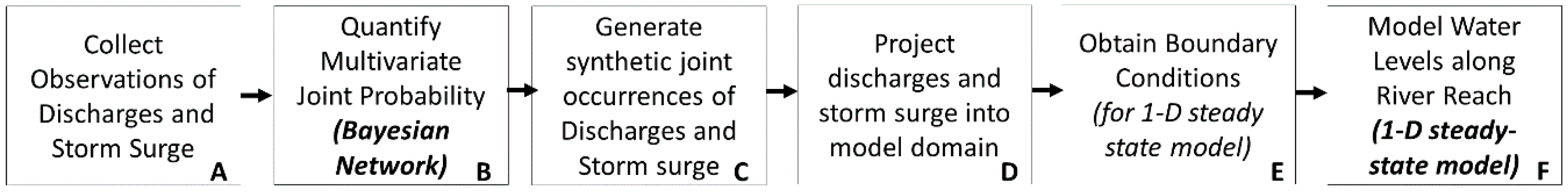
2. Materials and Methods

Figure 1 provides an overview of the framework applied in this paper. The BN was constructed based on daily observations of discharges in the coastal catchment and storm surge at the coast (box A in Figure 1). The BN model (box B) was extensively sampled to extract the equivalent of 500 years of daily joint realizations of discharges and storm surge (box C). After translating the storm surge at the coast to the mouth of the catchment and the tributary discharges to the main river reach (boxes D and E), we used these boundary conditions to force a 1D steady-state hydraulic model (box F). The modeled water surface profiles were analyzed and estimates of large return periods—up to a 500-year—were calculated and compared against empirical observations. We then tested the influence of spurious boundary conditions relationships on the delineation of the 100-year flood stage to better understand the importance of the multivariate statistical dependence on the water levels in the river reach.
The following section provides an overview of the theoretical background of the probabilistic model: the Bayesian Network (BN). A reader who is already familiar with Bayesian Networks may choose to give less attention to the next section and skip ahead to Section 2.2 which introduces the variables used to construct the BN, followed by an explanation of the methods (Section 2.3) and assumptions used in the hydraulic modeling (Section 2.4).

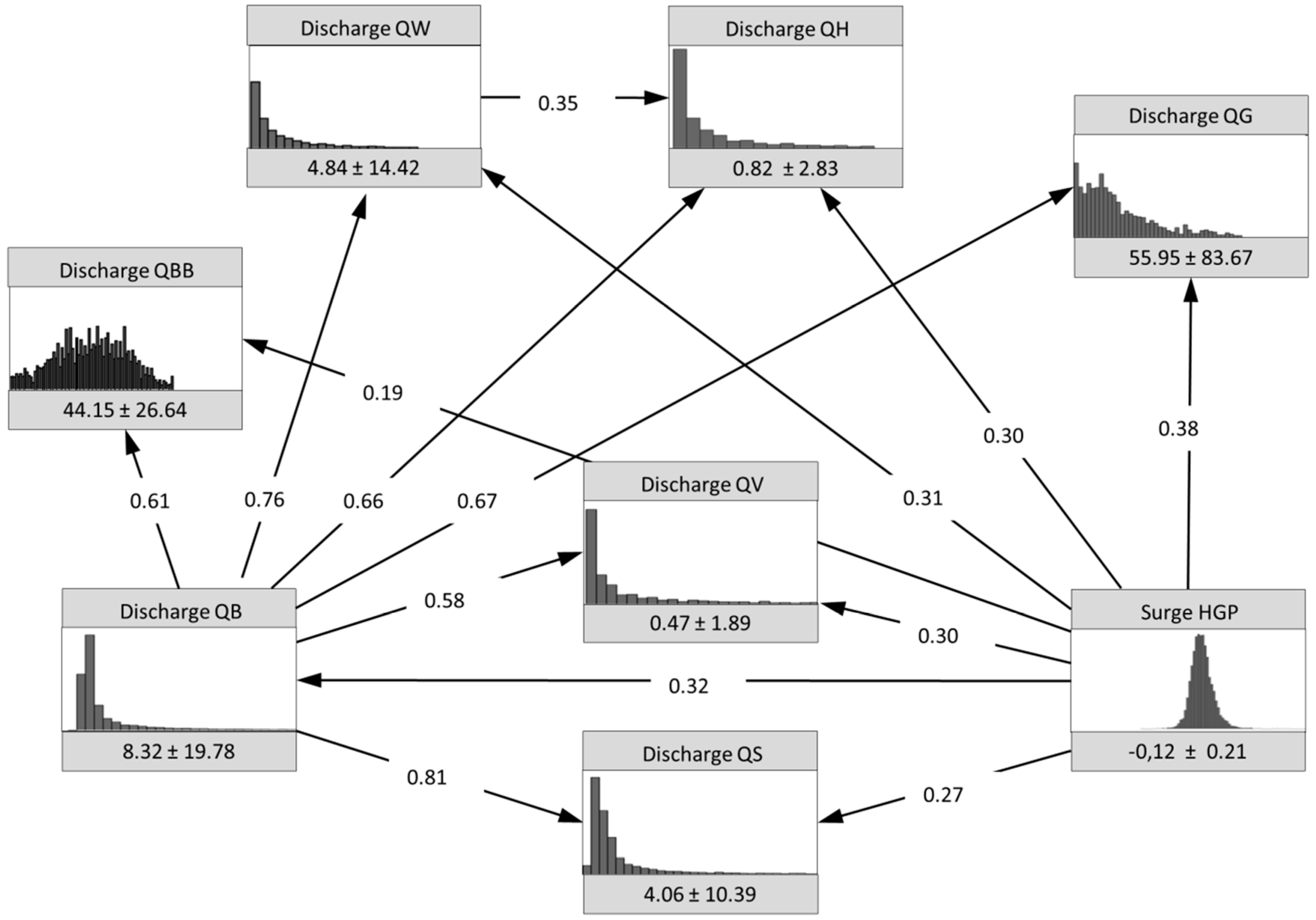
2.1. Bayesian Networks

Bayesian Networks (BNs) are probabilistic graphical models which explicitly include dependence between multiple random variables. Random variables are represented by nodes and connected by arcs forming a directed acyclic graph. The direction given to the arcs establish, in some cases, the causality structure and, in general, conditional independence statements between variables [49,50,51,52,53]. This structure determines which nodes are identified as parents of a given node, i.e., the predecessors, or as children, i.e., the successors. Variables can be discrete or continuous, and the expression of the (conditional) dependency is quantified by conditional probability functions. In this study, we will use the class of BNs described in Hanea et al. [52,53]. The joint density for BNs may be written as:
f X 1 ,   X 2 , , X n ( x 1 , x 2 , , x n ) = i = 1 n f X i Pa ( X i ) ( x i X Pa ( X i ) = x ) ,
where X Pa ( X i ) = x is short hand notation for X Pa 1 ( X i ) = x Pa 1 ( X i ) , , X Pa m ( X i ) = x Pa m ( X i ) and Pa ( X i ) is the set containing m parents of node X i . For nodes without parents, Pa ( X i ) = so that f X i Pa ( X i ) = f X i .
When only continuous variables are present in the model, the nodes representing the continuous random variables are usually constructed using their empirical distribution function, and the dependence structure between each pair of nodes is modeled using copulas. The use of copulas provides an efficient way to represent the joint probability and thus the dependence structure [54]. The advantage of copula functions is to separate the selection of an underlying multivariate distribution function from their one-dimensional marginal distributions. This enables a high flexibility in the representation of the multivariate dependence structure [28,54,55,56,57]. For the bivariate case, the cumulative distribution function, F X i X j ( x i ,   x j ) is defined as:
F X i X j ( x i ,   x j ) = C ( F X i ( x i ) ,   F X j ( x j ) ) = C ( u , v ) ,
where F X i ( x i ) and F X j ( x j ) are the marginal cumulative distribution functions, or uniform ranks, of the random variables X i and X j . C is the copula function and u and v are uniform variates on the unit square I   =   [ 0 , 1 ] 2 . We refer to References [58,59,60] for more theoretical background.
In the class of BNs used in this research, the multivariate dependence structure is parametrized with the empirical Spearman’s (conditional) rank correlation coefficient r between parent–child pairs and modeled using Gaussian copulas. The rank correlation coefficient is equivalent to the Pearson’s product moment correlation, ρ , applied to the ranks of the individual variables, such that:
r X i , X j = ρ ( F X i ( x i ) ,   F X j ( x j ) ) ,
Equation (3) is used to determine the parameter of the bivariate Gaussian copula, C ρ :
C ρ ( u , v ) = Φ ρ ( Φ 1 ( u ) ,   Φ 1 ( v ) ) ,
where Φ 1 is the inverse of the univariate standard normal distribution, and Φ ρ is the bivariate Gaussian cumulative distribution function. While the use of the Gaussian copula provides a computationally efficient formulation for sampling, in particular for large BN structures [52], it also restricts the representation of the dependence. Diagnostic tools (so-called informal tests) based on the Cramér-von-Mises statistic between alternative copulas and semi-correlation, as mentioned in Wang and Wells [61] and Joe [56], can provide some valuable guidance in the assessment of the fit of the bivariate data with respect to copula models. Formal hypothesis testing does not always lead to any valid model as a representation for a particular data set. Moreover, these tests may be very computationally expensive. For these reasons, we use both approaches as complementary. A description of these tests is given in Supplementary Material Section S5.2 and applied to the BN developed for this study.
It is beyond the scope of this paper to provide a complete overview of BNs. For more details on the class of BNs used in this paper, the reader is referred to Hanea et al. [52] and references therein. For our purpose, it is sufficient to say that, loosely, the BN to be used attaches: (1) either an empirical or parametric cumulative distribution function to the nodes representing random variables; (2) a non-unique assignment of (conditional) rank correlations to the arcs of the BN, and (3) a multivariate Gaussian copula that represents the dependence structure of the data and conditional independence structure dictated by the graph of the BN.
This class of Bayesian Networks has been successfully applied to various flood risk applications for different flood generating processes, namely to characterize extreme river discharge [62], to model expected riverine flood damages [50], and to estimate tropical cyclone parameters [5]. We extend their application further to generate stochastic boundary conditions which include compound flooding from riverine and coastal interactions and model their impact on a coastal catchment in Southeast Texas.

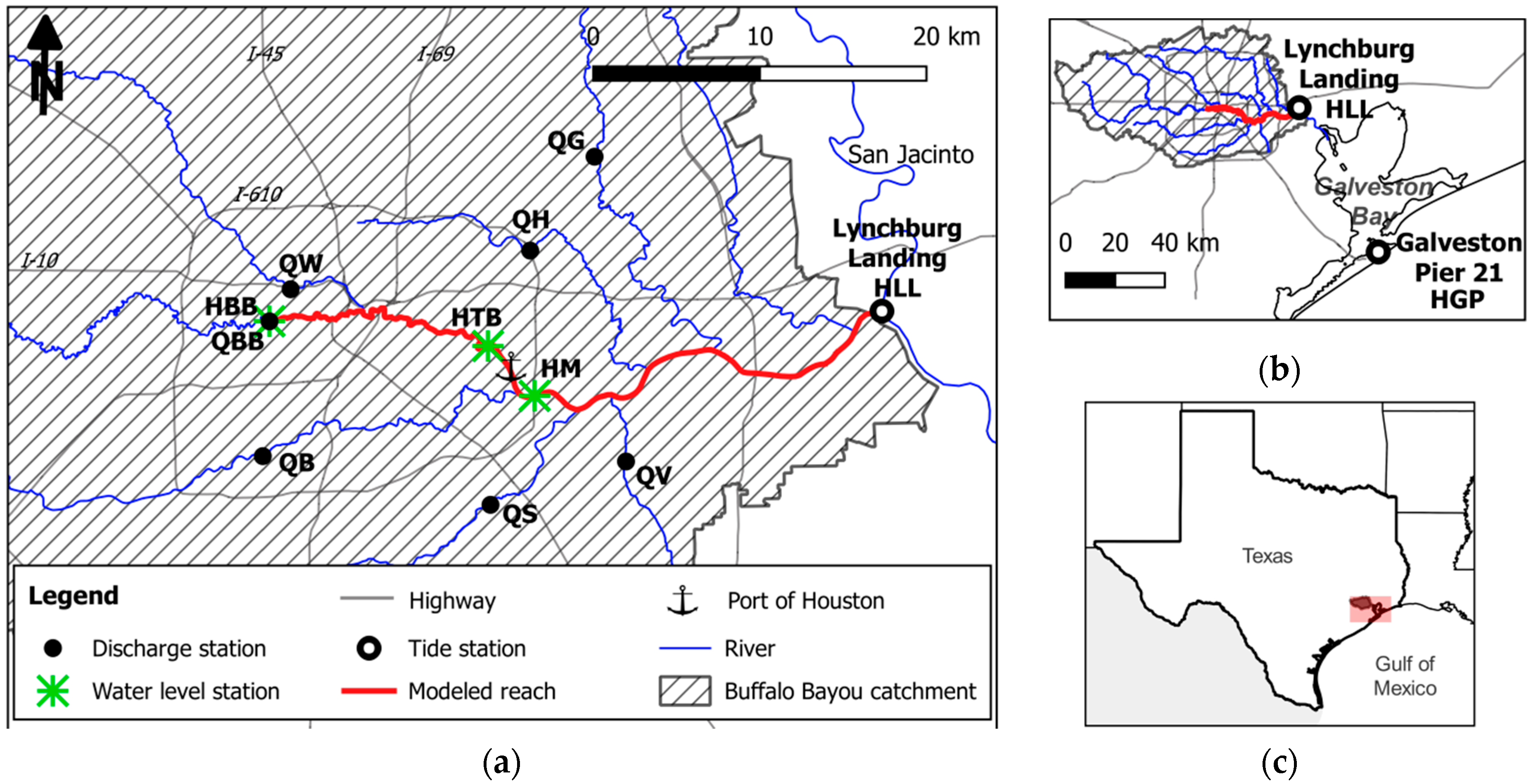
2.2. Data Collection

The location and characteristics of the Buffalo Bayou catchment make it prone to the co-occurrence of riverine and coastal floods. It is a small catchment (~2000 km2) exposed to intense rainfall events from local convective storms, large-scale frontal systems, and torrential rainfall brought by tropical cyclones. Historical records of flood events reported as major by the Federal Emergency Management Agency (FEMA) indicate a relatively equal importance of these different flood sources [18]. The response of the catchment to extreme rainfall has been further exacerbated by rapid development which has occurred over the century [63], leading to faster runoff rates and larger flood volumes [64,65].
This study focuses on characterizing water surface elevations along the downstream reach of Buffalo Bayou which flows through downtown Houston and the Port of Houston before joining the San Jacinto River, see Figure 2a. The catchment drains into Galveston Bay (Figure 2b), a shallow semi-enclosed estuary connected to the Gulf of Mexico via Bolivar Roads (Figure 2c). Buffalo Bayou upstream of the Port of Houston has a constant bed slope, approximately 0.55 m/km. Within the Port of Houston, the channel has the near-uniform bed slope of 0.12 m/km due to regular dredging to ensure sufficient ship clearance up to 14 m. Seven tributaries feed into the main stem of Buffalo Bayou before it reaches the Lynchburg Landing (LL) site.
Discharge: Mean daily discharges were collected from the U.S. Geological Survey at the locations shown in Figure 2a. The available period of data varied significantly per station, with records starting between 1936 and 1971. Abrupt changes in the discharge data series indicate a possible sign of anthropogenic influences on the hydrologic response of the catchment [66,67]. We identified the most important change in mean in the data series (function findchangepts() in MATLAB), which, at most stations, was found to be located between 1970 and 1980 (for details see Section S1.1 in Supplementary Material). Therefore, we selected data from 1 January 1980 onwards to represent the current developed state of the catchment and assumed stationary conditions between 1980 and 2016. Of the seven stations, four stations had a very high temporal coverage for this period (>97%), and three had a limited to poor coverage (9–43%).
Storm surge: Hourly water levels and astronomical tide projections were obtained from the National Oceanic and Atmospheric Administration (NOAA) for the LL and Galveston Pier 21 (GP) tide stations, Figure 2a,b. The LL tide station has a limited record length, about 11 years worth of data scattered between 1995 and 2014, compared to 113 years from 1904 to 2016 at GP. At both stations, hourly non-tidal residuals were calculated by subtracting the measured water level from the predicted astronomical tide. The maximum hourly non-tidal residuals in a day is set to be the daily non-tidal residual, what is referred to the storm surge in this study. Data for GP were further corrected for mean sea-level rise using a linear regression of the hourly non-tidal residuals of the whole record length, 1904–2016. This was not possible for the LL tide station, so we assumed stationarity of the available data.
For the sake of clarity, station IDs have been simplified. The original station numbers are provided in Section S1 in the Supplementary Material.

2.3. Bayesian Network Construction

The BN for the case study area was quantified based on the empirical marginal distributions of the daily discharges in the catchment (seven nodes) and the daily storm surge at GP (one node). A clear advantage of this choice is that the analysis of the statistical dependence gives insight into the physical mechanisms leading to flooding. However, in the case of strong serial dependence within the time series, this may lead to an incorrect quantification of the joint exceedance probability and therefore an underestimation of the flood hazard. Visual observations of the time series of the input variables showed that both coastal and river flood events are short-lived, from 1 to 2 days. To complement our visual findings, we investigated the presence of serial correlation based on the methodology presented in [68,69]. The results are presented in Section S3 of the Supplementary Material. In almost all cases except for two variables, the empirical autocorrelation functions dropped very rapidly below 0.1, indicating only a weak serial dependence. Therefore, we expected this effect to be of limited influence here and acknowledge that this choice may lead to conservative estimates of flood levels.
We used the Uninet software package (http://www.lighttwist.net/wp/uninet) to test various BN structures and extract the rank correlation matrix of the final model which is shown in Figure 3. Two discharge variables with a limited temporal coverage were inserted as user-defined random variables to maximize the number of joint observations from all nodes. This is further described in Section S5.1 in Supplementary Material. The BN was first constructed as a saturated graph and iteratively simplified by removing arcs with absolute conditional rank correlation lower than 0.3 (not shown here). All the arcs with the parent node ‘Surge HGP’ were kept to explicitly include the coastal and riverine interactions.
The Gaussian copula model was investigated against two alternative models, the Gumbel and Clayton copula, by comparing the Cramér-von-Mises statistic values as recommended in Reference [61] and semi-correlation [56]. Together, these copulas include a wide range of dependence observed in environmental data and express different types of tail dependence of importance when estimating extreme joint probabilities (Equation (S.3) in Supplementary Material and following discussion) [28,36,70,71]. We complemented these informal tests by a formal Goodness-of-Fit test [55] using two representative pair variables, discharge–discharge and surge–discharge. The detailed description of the tests and additional results are included in Sections S5.2 and S5.3 of Supplementary Material. The results highlight the difficulty of pinpointing a single copula model to capture the complexity of the joint behavior. Since the simplification of the dependence structure is inherent to the probabilistic model selected, we consider this choice as an additional source of uncertainty in the modeled water levels and perform a simple sensitivity analysis presented in the results section.
For the BN inference, we adopted a parametric representation of the marginal distribution since extreme values were of importance for this study. The BN inference was implemented with MATLAB [72] following a similar procedure described and developed by Hanea et al. [52] except for the inverse transformation of the uniform variables which relied on parametric marginal distributions presented next.
For the mean daily discharges, the marginal distributions were fitted with a parametrized distribution, the generalized extreme value (GEV) distribution which resulted in the lowest Akaike Information Criteria measure [73] among the 17 distribution candidates tested at each discharge station, except one where it ranked second. The GEV cumulative distribution, also referred as the Fisher-Tippet distribution, is:
F Q = exp { ( 1 + k ( x μ σ ) ) 1 k } ,
where x is a quantile of the discharge variable X , μ is the location parameter, σ the scale parameter, and k is the shape parameter with k 0 . We chose to specifically fit the upper tail of the data to put the emphasis on moderate to extreme discharge daily events and, therefore, used a truncated maximum-likelihood method to derive the distribution parameters (presented in Section S2.1 in Supplementary Material). A comparison against the regulatory riverine flood model provided little insight due to the difference in methodology applied which relies on a regression at the regional scale [18].
For the storm surge, the marginal distributions were fitted with a Gaussian mixture model with c = 2 components [74,75]:
f S = 1 c w j Φ ( · | μ j , σ j ) ,
where f S is the density probability function of the maximum hourly residual in a day, Φ ( · | μ j , σ j ) is the normal density with mean μ j and standard deviation σ j , and w j is the mixing coefficient of each component such that j w j = 1 and w j > 0 . The distribution parameters were estimated from the expectation maximization [75] and are presented in Table S2 of Supplementary Material. The 100-year water level was found to be 2.84 m-NAVD88, 95% bootstrap confidence interval [2.47, 3.13]. The extreme value analysis performed by NOAA [76] estimates this value to be 3.09 m-NAVD88 with a 95% confidence interval of [2.19, 4.89]. This comparison was not possible for the LL station since no return period estimates are mentioned for this station by NOAA.

2.4. 1D Hydraulic Model
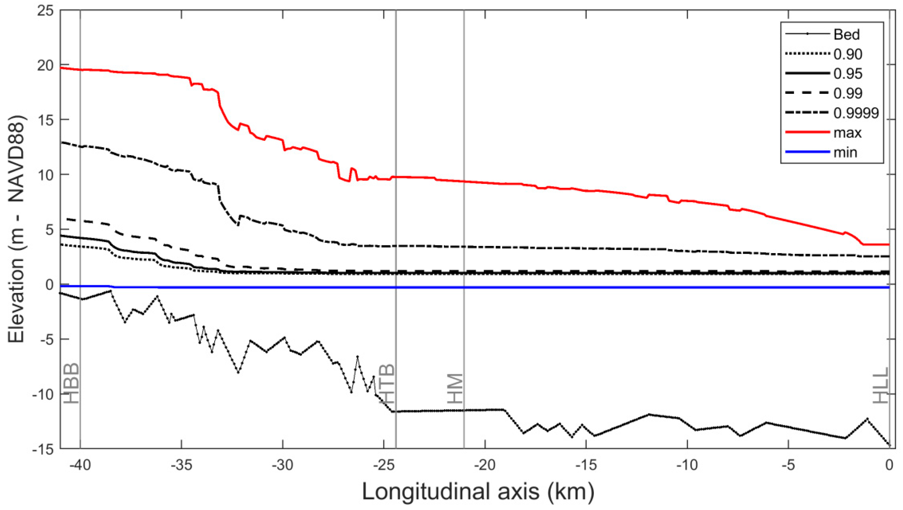
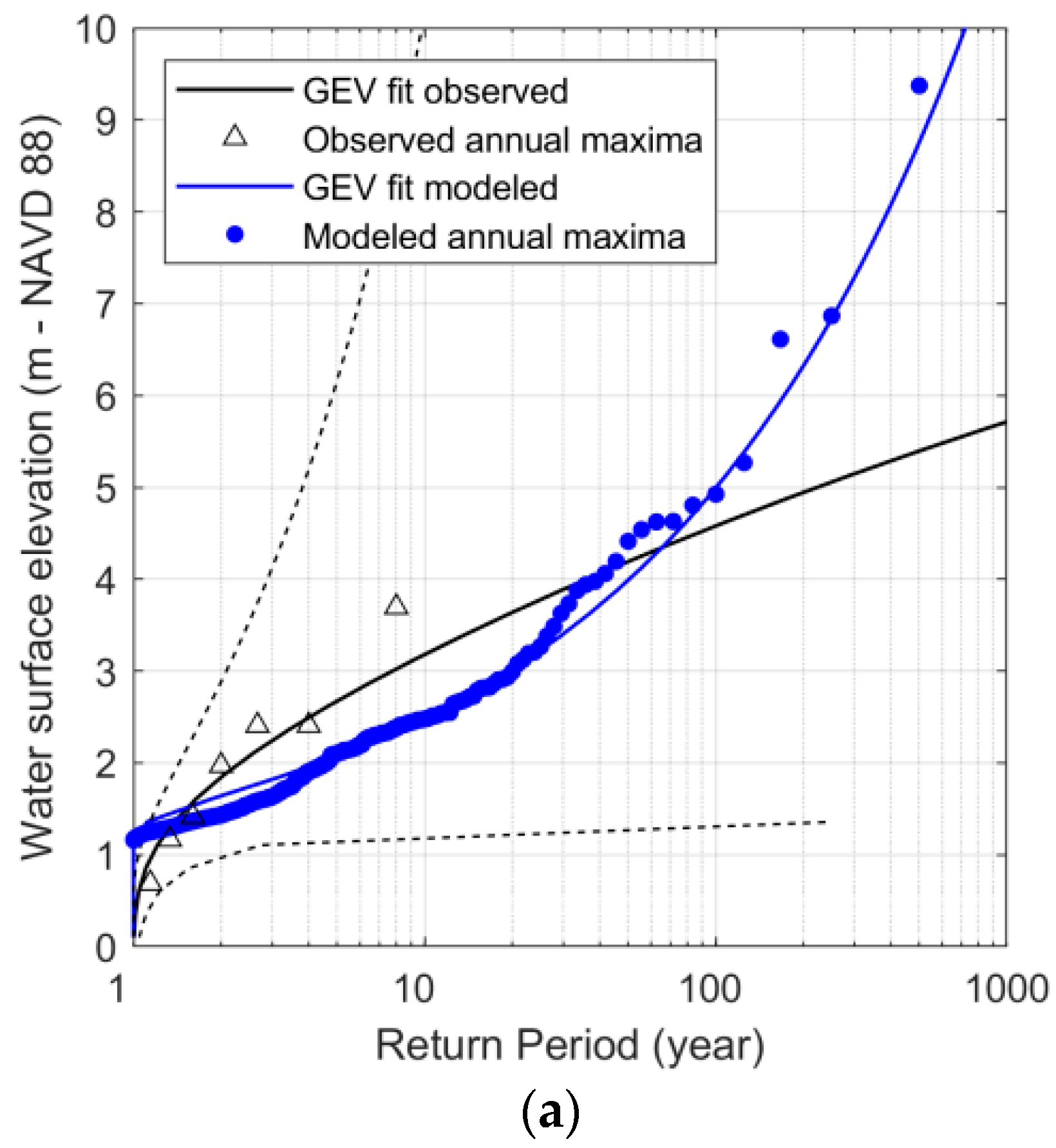
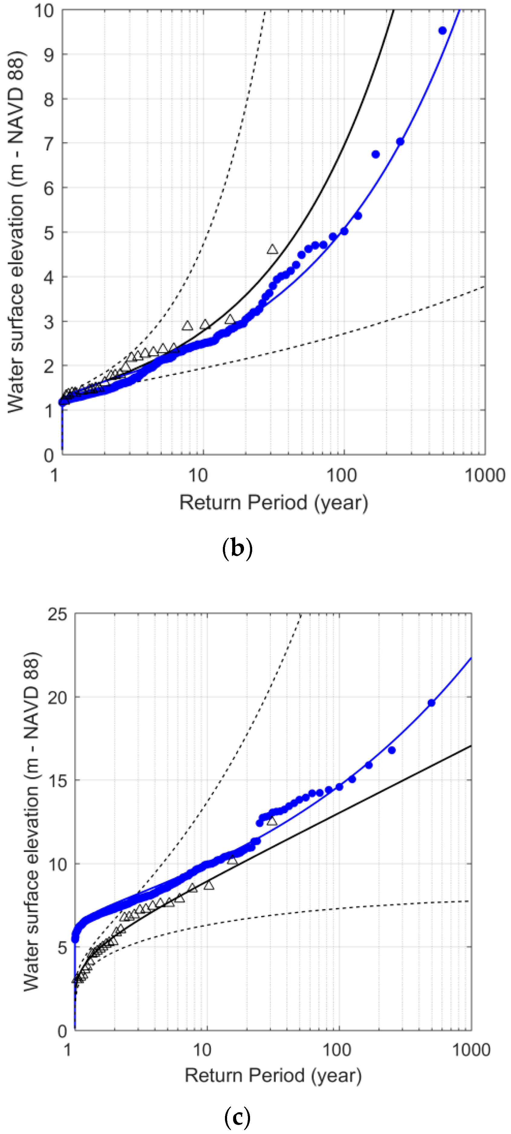
Longitudinal water profiles along the selected reach of Buffalo Bayou were obtained by solving the steady-state one-dimensional (1D) shallow water equations [77] with the standard step method [78] (as described in Section S4.1 in Supplementary Material). While this is a clear simplification of flood processes, water levels in the catchment are currently derived under similar assumptions to create the FEMA flood insurance rate maps (FIRMs) [18,26]. The spatial discretization was obtained from surveyed cross-sections [79] at approximately every kilometer, and the water surface elevations were calculated every 100 m, here forth referred to as river calculation points. The contributions from the tributaries were added as point sources along the river reach. Because the discharge stations do not cover the whole drainage area, discharge values were corrected based on an area-weighted average and lateral inflow was neglected. The downstream boundary condition at the LL site, i.e., the total water level, was reconstructed by adding the storm surge to the mean high tide level. The storm surge at LL was predicted based on the storm surge obtained for GP using a linear regression (Equation (S.1) in Supplementary Material). The hydraulic model was forced with the derived boundary conditions to obtain the water surface elevation along the selected reach.
The model showed a very good agreement with the 10-, 50-, 100- and 500-year return period riverine flood levels obtained from the validated Hydrologic Engineering Center’s River Analysis System (HEC-RAS) software model for Buffalo Bayou used to produce the aforementioned flood insurance maps (R2 > 0.98) [79]. Moreover, the model was also validated for Tropical Storm Frances (11 September 1998) and Tropical Storm Allison (6 June and 9 June 2001) and showed a reasonable performance, considering that water level observations from tropical cyclone events often have high uncertainty [80]. Results and figures from the runs are shown in Sections S4.2 and S4.3 in Supplementary Material.

3. Results

The BN model was sampled 182,500 times, equivalent to 500 years of daily observations, to generate possible realizations of daily discharge and storm surge from the multivariate joint distribution and model the resulting water surface elevations along the selected river reach. At each of the river calculation points, we extracted the 90th, 95th, 99th, and 99.99th percentile of the daily water level distribution, as shown in Figure 4. These percentiles are exceeded on average about 36, 18, 4 days per year, and once every 28 years, respectively. The maximum water surface elevation (red line in Figure 4) represents the highest water level obtained at each river calculation point from all the modeled daily joint occurrences of discharges and storm surge. Similarly, the minimum water surface elevation (blue line) indicates the lowest daily water surface elevation at each river calculation point. The model reproduces a wide range of conditions from extremely low to normal and extremely high water surface elevations.
We note that there is a nonlinear response in the propagation of the backwater effects on the water surface elevations modeled along the river reach. The imposed water level at the Lynchburg Landing site controls the water surface elevations in the downstream section, from approximately 0 to −25 km. As the bed slope steepens in the upstream section and the geometry of the river becomes more complex, the water surface elevations are determined by the backwater effects of the incoming tributary discharges along the river and the imposed downstream water level. As a result, there is a significant variation in the differences across all modeled scenarios between these two river sections. The range in modeled water levels is indicated by the difference between the minimum and maximum water surface elevation profiles. Upstream, this difference is about 20 m whereas downstream the difference is about 5 m. This shows that the magnitude of the backwater effects from the riverine and coastal interactions is influenced by the river characteristics which in turn determines the dominant flood drivers in the modeled water surface elevations.
We further focus on extreme water levels and characterize flood hazard at any location in the model domain by constructing annual exceedance probability curve from the modeled daily water surface elevations. We define the modeled ‘annual maxima’ of the water surface elevations by randomly separating the modeled water levels at each river calculation point into 500 bins of 365 days and extracting the maximum of each bin. By doing so, we assume the extreme modeled daily water surface elevations in the series to be independent of each other, which may lead to an overestimation of the flood level for a given annual exceedance probability. We compare our results at three locations along the river where observed annual maxima of water levels are present. Two stations, HM and HTB, are located close to each other in the Port of Houston, while the third station HBB, is located upstream. The exact location of the stations is indicated in Figure 1 and Figure 4. A GEV distribution is fitted to both the observed and modeled annual maxima data series, a commonly applied statistical distribution for the quantification of the probabilities of extreme water levels maxima [81,82,83].
Figure 5 shows the annual exceedance probability curves obtained from the model at the three locations where observations of annual maxima water levels are present. In general, the model is in agreement with the empirical return periods except at station HM (Figure 5a). When comparing Figure 5a,b, the model indicates a similar extreme value behavior while this is not the case for the empirical annual exceedance curves. This difference in extreme value behavior might be due to the uncertainties that stem from the discontinuous observed annual maxima series at station HM. Because the model framework outputs similar data series length, this contrast is absent, and a positive shape parameter is calculated at both locations, which is also consistent with the modeled hydraulic behavior. The performance of the hydraulic model also affects the results presented in Figure 5. Compared with the observed extreme water levels, the model underestimates extreme water surface elevations in the downstream reach (Figure 5b) and overestimates in the upstream reach (Figure 5c). In all cases, the annual exceedance probabilities of water levels are within the 95% confidence interval of the empirical distribution parameters, except in the high-frequency region for station HBB (Figure 5c).
To investigate the importance of the statistical dependence on the water levels in the river reach, we forced the hydraulic model with other joint boundary conditions derived independent of the BN model and compared them with the 100-year return period for each river calculation point obtained from the model framework. We selected two contrasting options often applied in large global flood hazard models, which we refer to as Case A and Case B:
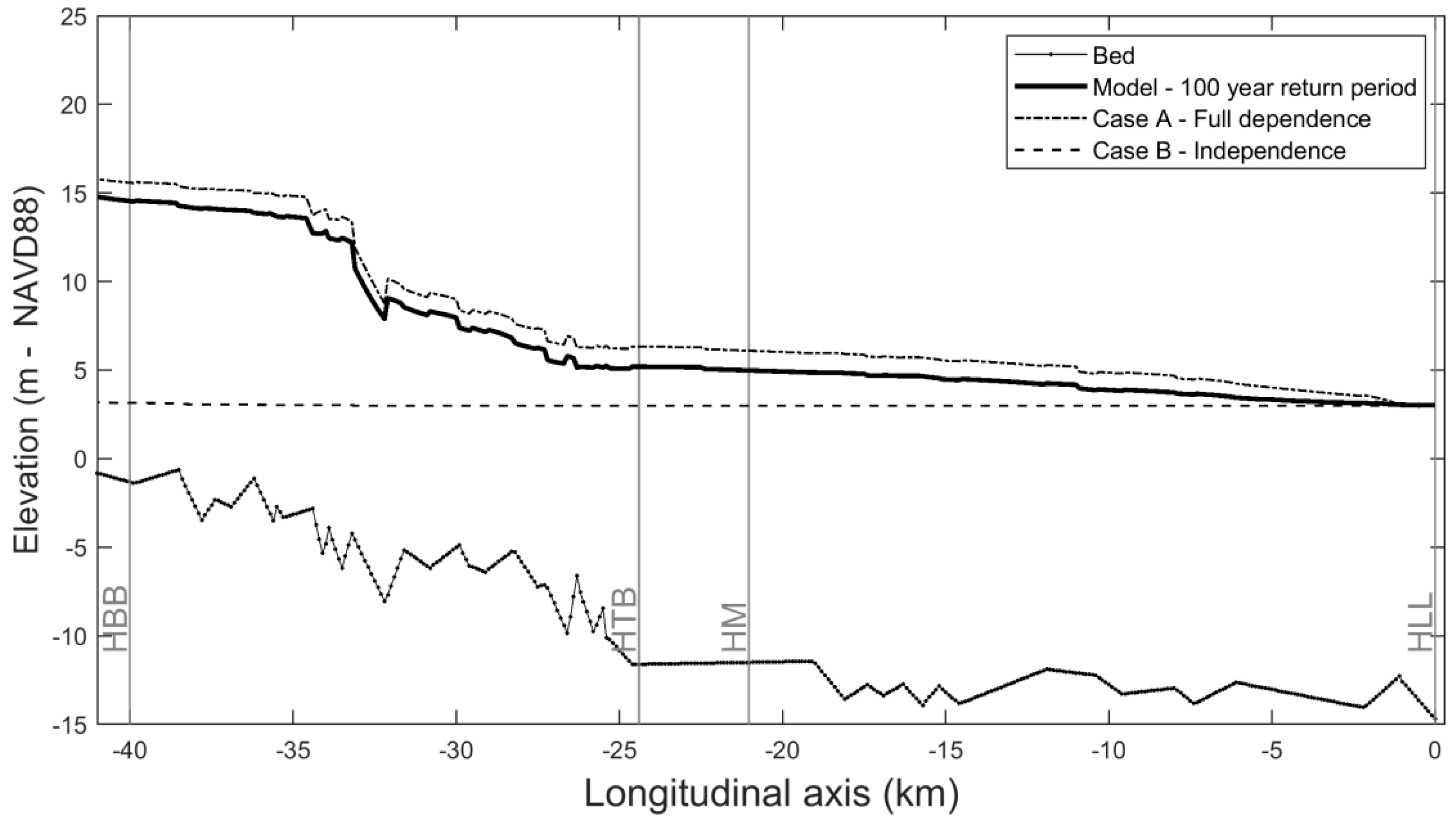
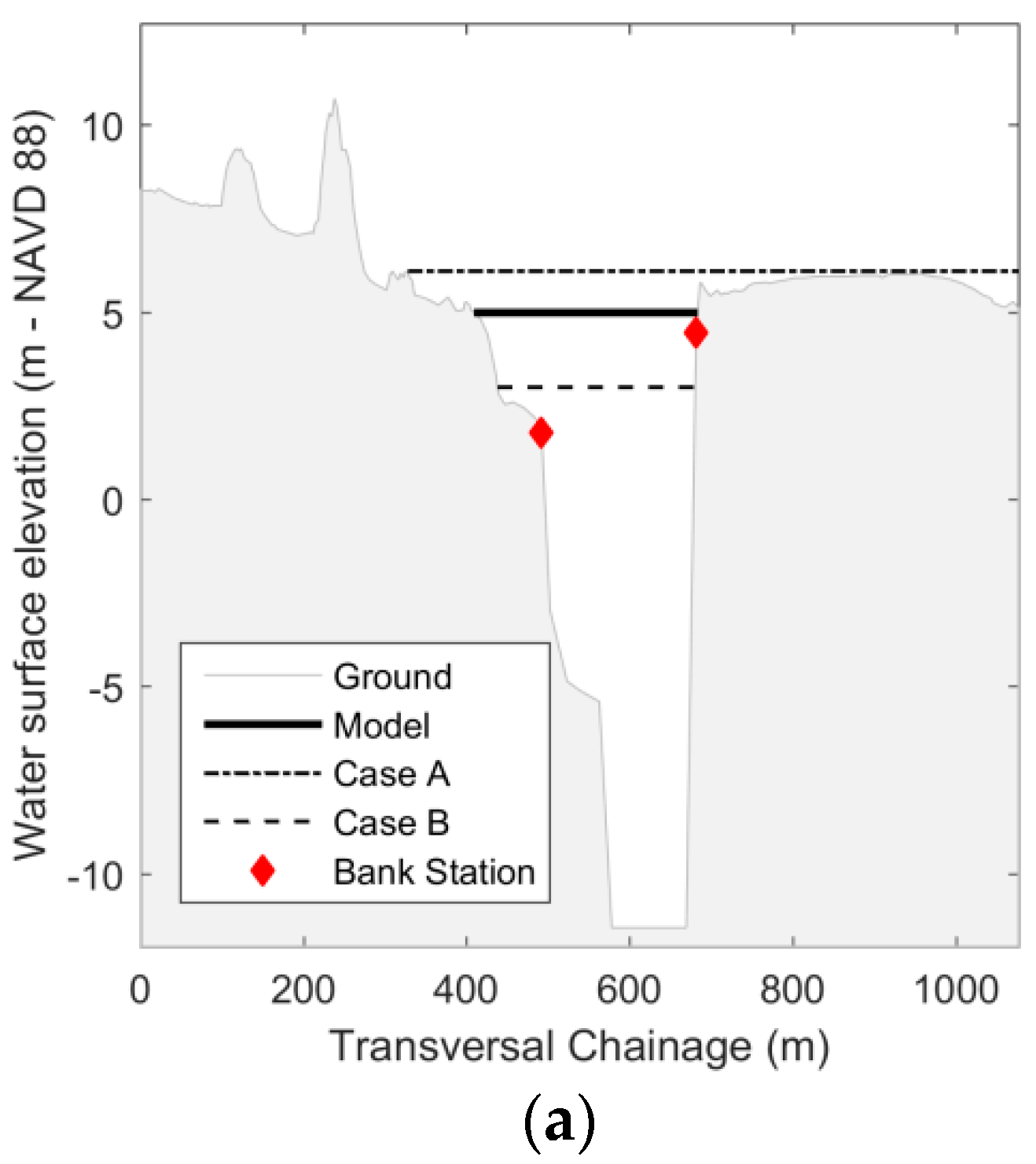
  • Case A: The 100-year marginal return period for each discharge variable and the storm surge variable is calculated and modeled. This represents the (untrue) assumption of full dependence.
  • Case B: The boundary conditions of the model are set to the marginal 100-year return period for the storm surge downstream, and the distribution mean for the upstream boundary conditions. This represents the (untrue) assumption of physical ‘independence’ between the downstream water level and the discharge. Such an approach is comparable to a bathtub approach [84], even though in the latter method discharges are usually completely neglected and not modeled.
As seen in Figure 6 and Figure 7, water surface elevations for Case A are higher than the 100-year return period obtained from the modeled outputs, with no difference at the Lynchburg Landing site and a 1 m difference within the rest of the river reach. This corresponds to a median relative error of 6.5%, with a maximum of 9.4%. The diagnostic tools presented in Sections S5.2 in Supplementary Material suggest that the joint dependence might deviate from the Gaussian copula model, especially between discharge variables. In the hypothetical case of upper tail dependence, accounting for this dependency relationship would result in the 100-year water level return period to be in between the curves obtained from the current model framework and Case A.
In contrast to Case A, Case B’s assumption leads to much higher differences in the model outputs. While we again observe no difference in water surface elevations at the Lynchburg Landing site, the difference increases moving upstream along the river and reaches a maximum difference of 12 m at the upstream end of the river reach. The median relative error is −12%, with a maximum of −75%. This result clearly highlights that neglecting discharge interactions can result in large underestimates of flood stage and, therefore, potential flood risks, especially upstream in the river reach.

4. Discussion

In this study, we used observations of mean daily discharge, daily storm surge, and their statistical dependence to generate stochastic joint occurrences of boundary conditions and model water surface elevations resulting from their interactions. Unlike previous studies, our model framework provides a method for characterizing the compound flood hazard along the entire river reach. Yet several limitations inherent to the construction of our model are present and discussed in this section, namely the simplification of the extreme flood events, the uncertainties in the BN generated from the lack of observations and the selection of the Gaussian copula and the assumption of stationarity in the flood hazard.
First, while the current model framework can capture a wide range of hydraulic conditions of relevance when studying compound events, it does not include the effect of flood duration on water surface elevations. The characteristics of both the riverine and coastal flood waves, such as volume and duration, determines when and where they will interact within the catchment. The analysis in Supplementary S3 confirmed that most flood events in the case study area tend to be short-lived. Yet, long flood events spanning multiple days have been observed in the catchment, such as Hurricane Harvey in August 2017. The tropical cyclone stalled over Texas generating extreme coastal water surface elevations and precipitation lasting for several days which impeded runoff from the system [85], causing critical road cutoffs, the release of toxic materials, and more than 70 fatalities [86,87]. Therefore, it is important to consider the temporal aspect of flood not only to correctly determine the flood hazard but also to properly model their impact on flood risk assessments.
Second, the lack of observations for three discharge variables (station QBB, QG, and QS) and for the storm surge at the Lynchburg Landing site introduces uncertainties in the quantification of their marginal distribution and of their statistical dependence with other variables in the BN, which propagate through the model framework. For example, we expect uncertainties in the water surface elevation imposed at the downstream boundary of the hydraulic model domain to strongly influence extreme water levels in the downstream reach. Wave contributions, such as wave setup and wave propagation, are also not directly represented by the BN but can strongly influence water levels [88,89,90]. While this study can be improved by using complementary data at these stations, this typically requires dedicated and extensive studies to properly capture complex coastal and hydrological processes [64,91,92] and is left for future studies.
Third, we restricted the multivariate dependence representation by relying on the Gaussian copula in the BN. However, our diagnostic tools indicated that especially for the pairs regarding discharges, asymmetries are present in the data which may not be captured adequately by the Gaussian copula (see Section S5.2 in Supplementary Material). Further research is needed to investigate the influence of the copula selection on the modeled water levels. Furthermore, the discharge data resolution leads to numerous repeated values for low discharges (as shown in Supplementary Figure S6b). The presence of ties can affect copula inference and parameter estimates [93]. Randomization procedures might be an option for further research [94]. A simple sensitivity test was conducted by assuming full dependence between the considered variables for the 100-year water level return period. We estimated the median relative error in water level along the river reach to be 6.5%, with a maximum of 9.4%. In future work, a comparison of the current BN model with a probabilistic model allowing for a higher flexibility in the selection of the dependence structure, such as Vine copula constructions [28], will help refine this result and better quantify the importance of the statistical dependence structure on the exceedance probability of high water levels due to compound flooding.
Finally, future flood hazards will be exacerbated by changes in environmental conditions and anthropogenic factors. Several recent publications have highlighted that climate change has increased precipitation in the study area [85,95]. Projected trends in urbanization in the United States also indicate a steady growth in urban land cover [96], which is expected to increase runoff peaks and volumes [97]. As a result, current estimates of flood hazard may become rapidly outdated [38]. This study provides a static characterization of the flood hazard, but future studies should use a modified framework and include such dynamics. This could be done, for example, by imposing a non-stationary parametric correlation coefficient [16,98] or by artificially shifting the marginal distribution [82,83].

5. Conclusions

In this paper, we presented a first attempt to characterize flood hazard in a coastal catchment prone to compound flooding from riverine and coastal interactions using a BN based on Gaussian copulas. We constructed and inferred the BN based on daily values of discharges and storm surge, and propagated the joint occurrences of discharges and storm surge to a hydraulic model to obtain the water level along Buffalo Bayou, in Southeast Texas. While uncertainties are introduced due to the selection of the Gaussian copula, the simplification in the hydraulic modeling and the limited data available for some variables, complex coastal and riverine interactions could be captured from the multivariate joint probability to characterize compound flood hazard along the whole model domain.
Because the BN is based on the statistical dependence, it provides a holistic procedure to stochastically derive joint boundary conditions while accounting for multivariate and spatial dependencies. The model framework generates daily water surface elevations resulting from various combinations of riverine and coastal conditions, including both moderate and extreme realizations, which is necessary for comprehensively analyzing the potential impacts of compound flood events. Moreover, the analysis of the modeled water levels underlined the importance of considering backwater effects due to high downstream water levels and tributary discharges. We also highlighted the effect of different spurious dependence assumptions between flood drivers on the modeled water level. We conclude that such differences can lead to an over—or underestimation of the annual exceedance probabilities when compared against measured dependence. Future work will focus on the characterization of flood hazard in diverse coastal catchments to better understand the propagation of flood drivers and their impact in the estuarine region in combination with other non-stationary drivers, such as relative sea-level rise and land cover changes.

Supplementary Materials

The following are available online at https://www.mdpi.com/2073-4441/10/9/1190/s1, Section S1: Data Collection, Section S2: Marginal Distribution Fit, Section S3: Autocorrelation function, Section S4: 1-D Hydraulic Model Performance, Section S5: Bayesian Network Construction and Validation. Figure S1: Available records of mean daily discharge for the stations of interests. The most important change in the mean is shown in red. Table S1/S2: GEV distribution parameters for the discharge/storm surge distributions. Figure S2: Autocorrelation function (ACF) at the stations of interests. Figures S3 and S4: Performance of the simplified hydraulic model developed for this study. Table S3: Semi-correlation and Cramér-von-Mises statistic for all variables used in the BN except for station QG, QS and QBB. Figure S5: Comparison of the maximum water levels observed for Tropical Storm Allison and Frances with the results from the 1-D hydraulic model. Figure S6: Selected examples of semi-correlation.

Author Contributions

Conceptualization, A.C., A.S. and O.M.-N.; Methodology, A.C., A.S. and O.M.-N.; Validation, A.C.; Writing-review and editing, A.C., A.S. and O.M.-N.; Visualization, A.C.

Funding

A.C. was supported by the Netherlands Organisation for Scientific Research (NWO) in the form of a VIDI grant (grant No. 016.161.324). A.S. was supported by the Netherlands America Foundation/Fulbright Fellowship for Water Management and the NSF PIRE Grant No. OISE-1545837.

Acknowledgments

The authors would like to thank H. Winsemius for his comments and suggestions during the writing of this manuscript. We would also like to thank three anonymous reviewers for their valuable comments which helped to improve this manuscript.

Conflicts of Interest

The authors declare no conflict of interest.

References

  1. Kron, W. Coasts: The high-risk areas of the world. Nat. Hazards 2013, 66, 1363–1382. [Google Scholar] [CrossRef]
  2. Rueda, A.; Camus, P.; Tomás, A.; Vitousek, S.; Méndez, F.J. A multivariate extreme wave and storm surge climate emulator based on weather patterns. Ocean Model. 2016, 104, 242–251. [Google Scholar] [CrossRef]
  3. Neumann, B.; Vafeidis, A.T.; Zimmermann, J.; Nicholls, R.J. Future coastal population growth and exposure to sea-level rise and coastal flooding—A global assessment. PLoS ONE 2015, 10. [Google Scholar] [CrossRef]
  4. Hallegatte, S.; Green, C.; Nicholls, R.J.; Corfee-Morlot, J. Future flood losses in major coastal cities. Nat. Clim. Chang. 2013, 3, 802–806. [Google Scholar] [CrossRef]
  5. Sebastian, A.; Dupuits, E.J.C.; Morales-Nápoles, O. Applying a Bayesian network based on Gaussian copulas to model the hydraulic boundary conditions for hurricane flood risk analysis in a coastal watershed. Coast. Eng. 2017, 125, 42–50. [Google Scholar] [CrossRef]
  6. Svensson, C.; Jones, D.A. Dependence between sea surge, river flow and precipitation in south and west Britain. Hydrol. Earth Syst. Sci. 2004, 8, 973–992. [Google Scholar] [CrossRef] [Green Version]
  7. Saleh, F.; Ramaswamy, V.; Wang, Y.; Georgas, N.; Blumberg, A.; Pullen, J. A Multi-Scale Ensemble-based Framework for Forecasting Compound Coastal-Riverine Flooding: The Hackensack-Passaic Watershed and Newark Bay. Adv. Water Resour. 2017, 110, 371–386. [Google Scholar] [CrossRef]
  8. Needham, H.F.; Keim, B.D.; Sathiaraj, D. A review of tropical cyclone-generated storm surges: Global data sources, observations, and impacts. Rev. Geophys. 2015, 53, 545–591. [Google Scholar] [CrossRef] [Green Version]
  9. Karl, T.R.; Melillo, J.M.; Peterson, T.C. Global Climate Change Impacts in the United States; Cambridge University Press: Cambridge, UK; New York, NY, USA, 2009; ISBN 9780521144070. [Google Scholar]
  10. Pielke, J.R.; Roger, A.; Gratz, J.; Landsea, C.W.; Collins, D.; Saunders, M.A.; Musulin, R. Normalized Hurricane Damage in the United States: 1900–2005. Nat. Hazards Rev. 2008, 9, 29–42. [Google Scholar] [CrossRef]
  11. Zheng, F.; Leonard, M.; Westra, S. Application of the design variable method to estimate coastal flood risk. J. Flood Risk Manag. 2015. [Google Scholar] [CrossRef]
  12. Klerk, W.J.; Winsemius, H.C.; van Verseveld, W.J.; Bakker, A.M.R.; Diermanse, F.L.M. The co-incidence of storm surges and extreme discharges within the Rhine–Meuse Delta. Environ. Res. Lett. 2015, 10, 035005. [Google Scholar] [CrossRef] [Green Version]
  13. Allen, G.H.; David, C.H.; Andreadis, K.M.; Hossain, F.; Famiglietti, J.S. Global Estimates of River Flow Wave Travel Times and Implications for Low-Latency Satellite Data. Geophys. Res. Lett. 2018. [Google Scholar] [CrossRef]
  14. Zscheischler, J.; Westra, S.; van den Hurk, B.J.J.M.; Seneviratne, S.I.; Ward, P.J.; Pitman, A.; AghaKouchak, A.; Bresch, D.N.; Leonard, M.; Wahl, T.; et al. Future climate risk from compound events. Nat. Clim. Chang. 2018, 8, 469–477. [Google Scholar] [CrossRef]
  15. Field, C.B.; Barros, V.; Stocker, T.F.; Dahe, Q.; Dokken, D.J.; Ebi, K.L.; Mastrandrea, M.D.; Mach, K.J.; Plattner, G.-K.; Allen, S.K.; et al. Managing the Risks of Extreme Events and Disasters to Advance Climate Change Adaptation. A Special Report of Working Groups I and II of the Intergovernmental Panel on Climate Change; Cambridge University Press: Cambridge, UK, 2012; ISBN 978-1-107-60780-4. [Google Scholar]
  16. Wahl, T.; Jain, S.; Bender, J.; Meyers, S.D.; Luther, M.E. Increasing risk of compound flooding from storm surge and rainfall for major US cities. Nat. Clim. Chang. 2015, 5, 1093–1097. [Google Scholar] [CrossRef]
  17. Federal Emergency Management Agency. Guidance for Flood Risk Analysis and Mapping; Combined Coastal and Riverine; Federal Emergency Management Agency: Washington, DC, USA, 2015. [Google Scholar]
  18. Federal Emergency Management Agency. Flood Insurance Study. Harris County, Texas and Incorporated Areas; Federal Emergency Management Agency: Washington, DC, USA, 2017; Volumes 1–2. [Google Scholar]
  19. Ward, P.; Jongman, B.; Salamon, P.; Simpson, A.; Bates, P.; De Groeve, T.; Muis, S.; de Perez, E.C.; Rudari, R.; Trigg, M.A.; Winsemius, H. Usefulness and limitations of global flood risk models. Nat. Clim. Chang. 2015, 5, 712–715. [Google Scholar] [CrossRef]
  20. Muis, S.; Verlaan, M.; Winsemius, H.C.; Aerts, J.C.J.H.; Ward, P.J. A global reanalysis of storm surges and extreme sea levels. Nat. Commun. 2016, 7, 11969. [Google Scholar] [CrossRef] [PubMed] [Green Version]
  21. Cid, A.; Camus, P.; Castanedo, S.; Méndez, F.J.; Medina, R. Global reconstructed daily surge levels from the 20th Century Reanalysis (1871–2010). Glob. Planet. Chang. 2017, 148, 9–21. [Google Scholar] [CrossRef]
  22. Vousdoukas, M.I.; Voukouvalas, E.; Mentaschi, L.; Dottori, F.; Giardino, A.; Bouziotas, D.; Bianchi, A.; Salamon, P.; Feyen, L. Developments in large-scale coastal flood hazard mapping. Nat. Hazards Earth Syst. Sci. 2016, 16, 1841–1853. [Google Scholar] [CrossRef] [Green Version]
  23. Winsemius, H.C.; Van Beek, L.P.H.; Jongman, B.; Ward, P.J.; Bouwman, A. A framework for global river flood risk assessments. Hydrol. Earth Syst. Sci. 2013, 17, 1871–1892. [Google Scholar] [CrossRef] [Green Version]
  24. Ward, P.; Jongman, B.; Weiland, F.; Bouwman, A.; van Beek, R.; Bierkens, M.; Ligtvoet, W.; Winsemius, H. Assessing flood risk at the global scale: Model setup, results, and sensitivity. Environ. Res. Lett. 2013, 8, 44019. [Google Scholar] [CrossRef] [Green Version]
  25. Maskell, J.; Horsburgh, K.; Lewis, M.; Bates, P. Investigating River-Surge Interaction in Idealised Estuaries. J. Coast. Res. 2014, 294, 248–259. [Google Scholar] [CrossRef]
  26. Ray, T.; Stepinski, E.; Sebastian, A.; Bedient, P.B. Dynamic Modeling of Storm Surge and Inland Flooding in a Texas Coastal Floodplain. J. Hydraul. Eng. 2011, 137, 1103–1111. [Google Scholar] [CrossRef]
  27. Kumbier, K.; Carvalho, R.C.; Vafeidis, A.T.; Woodroffe, C.D. Investigating compound flooding in an estuary using hydrodynamic modelling: A case study from the Shoalhaven River, Australia. Nat. Hazards Earth Syst. Sci. 2018, 2, 463–477. [Google Scholar] [CrossRef]
  28. Bevacqua, E.; Maraun, D.; Hobæk Haff, I.; Widmann, M.; Vrac, M. Multivariate statistical modelling of compound events via pair-copula constructions: analysis of floods in Ravenna (Italy). Hydrol. Earth Syst. Sci. 2017, 21, 2701–2723. [Google Scholar] [CrossRef] [Green Version]
  29. Zheng, F.; Leonard, M.; Westra, S. Efficient joint probability analysis of flood risk. J. Hydroinform. 2015, 17, 584–597. [Google Scholar] [CrossRef]
  30. Hawkes, P.J.; Gouldby, B.P.; Tawn, J.A.; Owen, M.W. The joint probability of waves and water levels in coastal engineering design. J. Hydraul. Res. 2002, 40, 241–251. [Google Scholar] [CrossRef]
  31. Leonard, M.; Westra, S.; Phatak, A.; Lambert, M.; van den Hurk, B.; Mcinnes, K.; Risbey, J.; Schuster, S.; Jakob, D.; Stafford-Smith, M.A. Compound event framework for understanding extreme impacts. Wiley Interdiscip. Rev. Clim. Chang. 2014, 5, 113–128. [Google Scholar] [CrossRef]
  32. Zheng, F.; Westra, S.; Leonard, M.; Sisson, S.A. Modeling dependence between extreme rainfall and storm surge to estimate coastal flooding risk. Water Resour. Res. 2014, 50, 2050–2071. [Google Scholar] [CrossRef] [Green Version]
  33. Kew, S.F.; Selten, F.M.; Lenderink, G.; Hazeleger, W. The simultaneous occurrence of surge and discharge extremes for the Rhine delta. Nat. Hazards Earth Syst. Sci. 2013, 13, 2017–2029. [Google Scholar] [CrossRef]
  34. Zheng, F.; Westra, S.; Sisson, S.A. Quantifying the dependence between extreme rainfall and storm surge in the coastal zone. J. Hydrol. 2013, 505, 172–187. [Google Scholar] [CrossRef]
  35. Ward, P.J.; Couasnon, A.; Eilander, D.; Haigh, I.; Hendry, A.; Muis, S.; Veldkamp, T.I.E.; Winsemius, H.; Wahl, T. Dependence between high sea-level and high river discharge increases flood hazard in global deltas and estuaries. Environ. Res. Lett. 2018. [Google Scholar] [CrossRef]
  36. Salvadori, G.; De Michele, C.; Kottegoda, N.T.; Rosso, R. Extremes in Nature: An Approach Using Copulas; Springer Science & Business Media: Berlin, Germany, 2007; pp. 1–294. ISBN 978-1-4020-4415-1. [Google Scholar]
  37. Salvadori, G.; Durante, F.; De Michele, C.; Bernardi, M.; Petrella, L. A multivariate copula-based framework for dealing with hazard scenarios and failure probabilities. Water Resour. Res. 2016, 52, 3701–3721. [Google Scholar] [CrossRef]
  38. Moftakhari, H.R.; Salvadori, G.; AghaKouchak, A.; Sanders, B.F.; Matthew, R.A. Compounding effects of sea level rise and fluvial flooding. Proc. Natl. Acad. Sci. USA 2017, 114, 9785–9790. [Google Scholar] [CrossRef] [PubMed] [Green Version]
  39. Van den Hurk, B.; van Meijgaard, E.; de Valk, P.; van Heeringen, K.-J.; Gooijer, J. Analysis of a compounding surge and precipitation event in the Netherlands. Environ. Res. Lett. 2015, 10, 035001. [Google Scholar] [CrossRef] [Green Version]
  40. Neal, J.; Keef, C.; Bates, P.; Beven, K.; Leedal, D. Probabilistic flood risk mapping including spatial dependence. Hydrol. Process. 2013, 27, 1349–1363. [Google Scholar] [CrossRef]
  41. Keef, C.; Tawn, J.A.; Lamb, R. Estimating the probability of widespread flood events. Environmetrics 2013, 24, 13–21. [Google Scholar] [CrossRef]
  42. Bender, J.; Wahl, T.; Müller, A.; Jensen, J. A multivariate design framework for river confluences. Hydrol. Sci. J. 2016, 61, 471–482. [Google Scholar] [CrossRef]
  43. Apel, H.; Thieken, A.H.; Merz, B.; Blöschl, G. Flood risk assessment and associated uncertainty. Nat. Hazards Earth Syst. Sci. 2004, 4, 295–308. [Google Scholar] [CrossRef] [Green Version]
  44. Lamb, R.; Keef, C.; Tawn, J.; Laeger, S.; Meadowcroft, I.; Surendran, S.; Dunning, P.; Batstone, C. A new method to assess the risk of local and widespread flooding on rivers and coasts. J. Flood Risk Manag. 2010, 3, 323–336. [Google Scholar] [CrossRef]
  45. Port of Houston Authority. Available online: http://www.porthouston.com/ (accessed on 27 March 2018).
  46. Davlasheridze, M.; Atoba, K.O.; Brody, S.; Highfield, W.; Merrell, W.; Ebersole, B.; Purdue, A.; Gilmer, R.W. Economic impacts of storm surge and the cost-benefit analysis of a coastal spine as the surge mitigation strategy in Houston-Galveston area in the USA. Mitig. Adapt. Strateg. Glob. Chang. 2018, 1–26. [Google Scholar] [CrossRef]
  47. Christian, J.; Fang, Z.; Torres, J.; Deitz, R.; Bedient, P. Modeling the Hydraulic Effectiveness of a Proposed Storm Surge Barrier System for the Houston Ship Channel during Hurricane Events. Nat. Hazards Rev. 2015, 16, 04014015. [Google Scholar] [CrossRef]
  48. Torres, J.M.; Bass, B.; Irza, J.N.; Proft, J.; Sebastian, A.; Dawson, C.; Bedient, P. Modeling the Hydrodynamic Performance of a Conceptual Storm Surge Barrier System for the Galveston Bay Region. J. Waterw. Port Coast. Ocean Eng. 2017, 143, 05017002. [Google Scholar] [CrossRef]
  49. Niedermayer, D. An Introduction to Bayesian Networks and Their Contemporary Applications; Innovations in Bayesian Networks; Springer: Berlin/Heidelberg, Germany, 2008; pp. 117–130. ISBN 9783540850656. [Google Scholar]
  50. Vogel, K.; Riggelsen, C.; Korup, O.; Scherbaum, F. Bayesian network learning for natural hazard analyses. Nat. Hazards Earth Syst. Sci. 2014, 14, 2605–2626. [Google Scholar] [CrossRef] [Green Version]
  51. Weber, P.; Medina-Oliva, G.; Simon, C.; Iung, B. Overview on Bayesian networks applications for dependability, risk analysis and maintenance areas. Eng. Appl. Artif. Intell. 2012, 25, 671–682. [Google Scholar] [CrossRef]
  52. Hanea, A.; Morales Napoles, O.; Ababei, D. Non-parametric Bayesian networks: Improving theory and reviewing applications. Reliab. Eng. Syst. Saf. 2015, 144, 265–284. [Google Scholar] [CrossRef]
  53. Hanea, A.M.; Kurowicka, D.; Cooke, R.M. Hybrid Method for Quantifying and Analyzing Bayesian Belief Nets. Qual. Reliab. Eng. Int. 2006, 22, 709–729. [Google Scholar] [CrossRef]
  54. Salvadori, G.; De Michele, C. Frequency analysis via copulas: Theoretical aspects and applications to hydrological events. Water Resour. Res. 2004, 40, 1–17. [Google Scholar] [CrossRef]
  55. Genest, C.; Favre, A.-C. Everything You Always Wanted to Know about Copula Modeling but Were Afraid to Ask. J. Hydrol. Eng. 2007, 12, 347–368. [Google Scholar] [CrossRef] [Green Version]
  56. Joe, H. Dependence Modeling with Copulas; Chapman & Hall/CRC: London, UK, 2015; ISBN 9781466583221. [Google Scholar]
  57. Graler, B.; Van Den Berg, M.J.; Vandenberghe, S.; Petroselli, A.; Grimaldi, S.; De Baets, B.; Verhoest, N.E.C. Multivariate return periods in hydrology: A critical and practical review focusing on synthetic design hydrograph estimation. Hydrol. Earth Syst. Sci. 2013, 17, 1281–1296. [Google Scholar] [CrossRef] [Green Version]
  58. Sklar, A. Fonctions de répartition à n dimensions et leurs marges. Publ. Inst. Stat. Univ. Paris 1959, 8, 229–231. [Google Scholar]
  59. Nelsen, R.B. An Introduction to Copulas, 2nd ed.; Springer Science & Business Media: New York, NY, USA, 2006. [Google Scholar]
  60. Joe, H. Multivariate Models and Multivariate Dependence Concepts; CRC Press: London, UK, 1997. [Google Scholar]
  61. Wang, W.; Wells, M.T. Model Selection and Semiparametric Inference for Bivariate Failure-Time Data. J. Am. Stat. Assoc. 2000, 95, 62–72. [Google Scholar] [CrossRef]
  62. Paprotny, D.; Morales-Nápoles, O. Estimating extreme river discharges in Europe through a Bayesian network. Hydrol. Earth Syst. Sci. 2017, 21, 2615–2636. [Google Scholar] [CrossRef] [Green Version]
  63. Qian, Z. Without zoning: Urban development and land use controls in Houston. Cities 2010, 27, 31–41. [Google Scholar] [CrossRef]
  64. Gori, A.; Blessing, R.; Juan, A.; Brody, S.; Bedient, P. Characterizing urbanization impacts on floodplain through integrated land use, hydrologic, and hydraulic modeling. J. Hydrol. 2018, in press. [Google Scholar]
  65. Gori, A. Quantifying Impacts of Development on Floodplain Evolution and Projection of Future Flood Hazard: Applications to Harris County. Master’s Thesis, Rice University, Houston, TX, USA, 2018. [Google Scholar]
  66. Mallakpour, I.; Villarini, G. The changing nature of flooding across the central United States. Nat. Clim. Chang. 2015, 5, 250–254. [Google Scholar] [CrossRef]
  67. Villarini, G.; Smith, J.A.; Baeck, M.L.; Krajewski, W.F. Examining Flood Frequency Distributions in the Midwest US. JAWRA J. Am. Water Resour. Assoc. 2011, 47, 447–463. [Google Scholar] [CrossRef]
  68. Serinaldi, F. Can we tell more than we can know? The limits of bivariate drought analyses in the United States. Stoch. Environ. Res. Risk Assess. 2015, 30, 1691–1704. [Google Scholar] [CrossRef]
  69. Claps, P.; Laio, F. Can continuous streamflow data support flood frequency analysis? An alternative to the partial duration series approach. Water Resour. Res. 2003, 39, 1–11. [Google Scholar] [CrossRef]
  70. Hobaek Haff, I.; Frigessi, A.; Maraun, D. How well do regional climate models simulate the spatial dependence of precipitation? An application of pair-copula constructions. J. Geophys. Res. D Atmos. 2015, 120, 2624–2646. [Google Scholar] [CrossRef] [Green Version]
  71. Serinaldi, F.; Bárdossy, A.; Kilsby, C.G. Upper tail dependence in rainfall extremes: would we know it if we saw it? Stoch. Environ. Res. Risk Assess. 2015, 29, 1211–1233. [Google Scholar] [CrossRef]
  72. Morales-Nápoles, O.; Worm, D.; van den Haak, P.; Hanea, A.; Courage, W.; Miraglia, S. Reader for Course: Introduction to Bayesian Networks; TNO-060-DTM-2013-01115; TNO: Delft, The Netherlands, 2013. [Google Scholar]
  73. Mutua, F.M. The use of the Akaike Information Criterion in the identification of an optimum flood frequency model. Hydrol. Sci. J. 1994, 39, 235–244. [Google Scholar] [CrossRef] [Green Version]
  74. Morales-Nápoles, O.; Steenbergen, R.D.J.M. Large-Scale Hybrid Bayesian Network for Traffic Load Modeling from Weigh-in-Motion System Data. J. Bridg. Eng. 2014, 20, 1–10. [Google Scholar] [CrossRef]
  75. McLachlan, G.; Peel, D. Finite Mixture Models; Wiley Interscience: Hoboken, NJ, USA, 2000. [Google Scholar]
  76. NOAA National Oceanic and Atmospheric Administration. Tides and Currents. Annual Exceedance Probability Curves 8771450 Galveston Pier 21, TX. Available online: https://tidesandcurrents.noaa.gov/est/curves.shtml?stnid=8771450 (accessed on 15 December 2017).
  77. Henderson, F.M. Open Channel Flow; Prentice-Hall: Upper Saddle River, NJ, USA, 1966; ISBN 0023535105. [Google Scholar]
  78. Brunner, G.W. HEC-RAS River Analysis System. Hydraulic Reference Manual; US Army Corps of Engineers, Institute for Water Resources, Hydrologic Engineering Center: Davis, CA, USA, 2016. [Google Scholar]
  79. Harris County Flood Control District Model and Map Management System. Available online: http://www.m3models.org/ (accessed on 1 July 2016).
  80. Landsea, C.W.; Franklin, J.L. Atlantic Hurricane Database Uncertainty and Presentation of a New Database Format. Mon. Weather Rev. 2013, 141, 3576–3592. [Google Scholar] [CrossRef]
  81. Arns, A.; Wahl, T.; Haigh, I.D.; Jensen, J.; Pattiaratchi, C. Estimating extreme water level probabilities: A comparison of the direct methods and recommendations for best practise. Coast. Eng. 2013, 81, 51–66. [Google Scholar] [CrossRef]
  82. Arns, A.; Dangendorf , S.; Jensen, J.; Talke, S.; Bender, J.; Pattiaratchi, C. Sea-level rise induced amplification of coastal protection design heights. Sci. Rep. 2017, 7, 40171. [Google Scholar] [CrossRef] [PubMed] [Green Version]
  83. Vitousek, S.; Barnard, P.L.; Fletcher, C.H.; Frazer, N.; Erikson, L.; Storlazzi, C.D. Doubling of coastal flooding frequency within decades due to sea-level rise. Sci. Rep. 2017, 7, 1399. [Google Scholar] [CrossRef] [PubMed]
  84. Teng, J.; Jakeman, A.J.; Vaze, J.; Croke, B.F.W.; Dutta, D.; Kim, S. Flood inundation modelling: A review of methods, recent advances and uncertainty analysis. Environ. Model. Softw. 2017, 90, 201–216. [Google Scholar] [CrossRef]
  85. Van Oldenborgh, G.J.; van der Wiel, K.; Sebastian, A.; Singh, R.; Arrighi, J.; Otto, F.; Haustein, K.; Li, S.; Vecchi, G.; Cullen, H. Attribution of extreme rainfall from Hurricane Harvey, August 2017. Environ. Res. Lett. 2017, 12, 124009. [Google Scholar] [CrossRef] [Green Version]
  86. Sebastian, A.G.; Lendering, K.T.; Kothuis, B.L.M.; Brand, A.D.; Jonkman, S.N. Hurricane Harvey Report. A Fact-Finding Effort in the Direct Aftermath of Hurricane Harvey in the Greater Houston Region; Delft University Publishers: Delft, The Netherlands, 2017. [Google Scholar]
  87. Jonkman, S.N.; Godfroy, M.; Sebastian, A.; Kolen, B. Brief communication: Post-event analysis of loss of life due to hurricane Harvey. Nat. Hazards Earth Syst. Sci. 2018, 18, 1073–1078. [Google Scholar] [CrossRef]
  88. Serafin, K.A.; Ruggiero, P.; Stockdon, H.F. The relative contribution of waves, tides, and nontidal residuals to extreme total water levels on U.S. West Coast sandy beaches. Geophys. Res. Lett. 2017, 44, 1839–1847. [Google Scholar] [CrossRef]
  89. Vousdoukas, M.I.; Bouziotas, D.; Giardino, A.; Bouwer, L.M.; Mentaschi, L.; Feyen, L. Understanding epistemic uncertainty in large-scale coastal flood risk assessment for present and future climates. Nat. Hazards Earth Syst. Sci. 2018, 18, 2127–2142. [Google Scholar] [CrossRef]
  90. Melito, L.; Postacchini, M.; Sheremet, A.; Calantoni, J.; Zitti, G.; Darvini, G.; Brocchini, M. Wave-Current Interactions and Infragravity Wave Propagation at a Microtidal Inlet. Proceedings 2018, 2, 628. [Google Scholar] [CrossRef]
  91. Sebastian, A.; Proft, J.; Dietrich, J.C.; Du, W.; Bedient, P.B.; Dawson, C.N. Characterizing hurricane storm surge behavior in Galveston Bay using the SWAN+ADCIRC model. Coast. Eng. 2014, 88, 171–181. [Google Scholar] [CrossRef]
  92. Dietrich, J.C.; Zijlema, M.; Westerink, J.J.; Holthuijsen, L.H.; Dawson, C.; Luettich, R.A.; Jensen, R.E.; Smith, J.M.; Stelling, G.S.; Stone, G.W. Modeling hurricane waves and storm surge using integrally-coupled, scalable computations. Coast. Eng. 2011, 58, 45–65. [Google Scholar] [CrossRef]
  93. Salvadori, G.; Tomasicchio, G.R.; D’Alessandro, F. Practical guidelines for multivariate analysis and design in coastal and off-shore engineering. Coast. Eng. 2014, 88, 1–14. [Google Scholar] [CrossRef]
  94. Pappadà, R.; Durante, F.; Salvadori, G. Quantification of the environmental structural risk with spoiling ties: Is randomization worthwhile? Stoch. Environ. Res. Risk Assess. 2017, 31, 2483–2497. [Google Scholar] [CrossRef]
  95. Emanuel, K. Assessing the present and future probability of Hurricane Harvey’s rainfall. Proc. Natl. Acad. Sci. USA 2017, 201716222. [Google Scholar] [CrossRef] [PubMed]
  96. Hamilton, C.M.; Martinuzzi, S.; Plantinga, A.J.; Radeloff, V.C.; Lewis, D.J.; Thogmartin, W.E.; Heglund, P.J.; Pidgeon, A.M. Current and Future Land Use around a Nationwide Protected Area Network. PLoS ONE 2013, 8. [Google Scholar] [CrossRef] [PubMed] [Green Version]
  97. Hollis, G.E. The effect of urbanization on floods of different recurrence interval. Water Resour. Res. 1975, 11, 431–435. [Google Scholar] [CrossRef]
  98. Sarhadi, A. Time-varying nonstationarymultivariate risk analysis using a dynamic Bayesian copula. Water Resour. Res. 2016, 52, 2327–2349. [Google Scholar] [CrossRef]
Figure 1. Schematic workflow for generating stochastic water surface profiles in a coastal catchment.
Water 10 01190 g001
Figure 2. Location of the case study area, the Buffalo Bayou catchment (a) which drains into the Galveston Bay (b) and connected to the Gulf of Mexico (c). The discharge stations (filled circles in black) and the tide station (empty circles) Galveston Pier 21 are used to construct the BN and model water surface elevations along the main stem of the Buffalo Bayou catchment (red line). Water level stations (green) were used for the comparison with the modeled extreme water levels.
Water 10 01190 g002
Figure 3. The Bayesian Network model for the Buffalo Bayou catchment. The boxes represent the nodes and the arrows the arcs. The values of the (conditional) rank correlation coefficient are shown on each arc. The histogram in the node shows the empirical probability distribution function for each variable and the values below represent the mean and standard deviation, respectively. Units are in m3s-1 for discharge and in m for the storm surge.
Water 10 01190 g003
Figure 4. Maximum (red), minimum (blue) water surface elevations and percentiles (90th, 95th, 99th, and 99.99th) of daily water levels at each river calculation point obtained by inferring the BN 182,500 times and modeling the resulting water surface profile.
Water 10 01190 g004
Figure 5. Comparison of the annual exceedance probability distributions from observed and modeled annual maxima at stations HM (a), HTB (b) and HBB (c). The dashed lines indicate the fit of the 95% confidence interval from the empirical GEV distribution parameters. The stations are presented from downstream to upstream along the Buffalo Bayou river, with stations HM and HTB located in the Port of Houston, see also Figure 1 and Figure 4 for their exact location.
Water 10 01190 g005aWater 10 01190 g005b
Figure 6. Sensitivity of the multivariate dependence assumptions. The 100–year water level obtained from the current model framework is represented by the black full line. Case A and B represent full dependence and ‘independence’ of the boundary conditions, respectively (see text).
Water 10 01190 g006
Figure 7. Similar to Figure 6 but in the transverse direction at stations HM (a), HTB (b) and HBB (c). The location of the bank stations is extracted from the regulatory HEC-RAS riverine flood model and roughly indicates the change in channel conveyance.
Water 10 01190 g007aWater 10 01190 g007b

