Numerical Simulation of Gate Control for Unsteady Irrigation Flow to Improve Water Use Efficiency in Farming

Abstract

In the case of irrigation, to implement the water distribution plan, the flow needs to be changed through the gate which leads to the occurrence of unavoidable unsteady flow. In order to improve the level of irrigation management, it is necessary to understand the changes taking place in the canal water flow during the process of water distribution. The de Saint-Venant equations were solved based on the method of characteristics and a model was built to simulate the unsteady flow in the channel of the Yintang irrigation district. Then, the obtained results were validated by the employed model. On the basis of simulation results, a model for the variations in the gate opening was established based on the theory of under-gate discharge. In this study, the simulation results, as established from the model, are very consistent with the simulation results of existing commercial software and a simple design for the operation was conducted from the adjustment of gate openings and multi-stage gate operation modes. Overall, the established gate control model built in this study is reliable, which provides a basis for the decision-making process for the relevant staff.

1. Introduction

China is a large agricultural country and protecting the usage of water in agriculture is the basis for ensuring the national economy as well as the foundation for sustained economic development [1]. The existing irrigated area of China is 66 million ha, and agricultural water accounts for 62.4% of the total water usage [2]. At present, the problem of shortage of water resources in China is very serious and has become one of the important factors restricting China’s economic and social development. Therefore, in order to deal with water crisis, it is necessary to adopt measures of water-saving in the agriculture. When the irrigation channel system is used for water distribution, it needs to be adjusted by the gate according to the water requirement of the irrigation area. At this time, the flow in the channel is disturbed and an unsteady flow occurs, so that there are changes in the water level and discharge in the channel with time. Due to the inability to predict this transition process, repeated scheduling often occurs which leads to poor reliability and accuracy of water distribution channels, wasting of water, and reduced irrigation quality. In order to make the entire channel system scientific and rational in the process of water diversion, water conveyance and water distribution, reducing the loss of water from the channel improves the efficiency of water use and achieves the purpose of water conservation, where numerical simulation plays a key role and is the most effective and feasible method.

The theoretical study of unsteady flow in open channels originated from the study of shallow water waves by Laplace and Lagrange in the late eighteenth century, following which Lagrange derived an equation for wave velocity. In 1871, de Saint-Venant proposed the theory and general equations for the unsteady flow of open channels, namely the de Saint-Venant equations, and thus the phenomenon of unsteady flow in open channels can be described mathematically. Stoker [3], as the forerunner of explicit methods for solving equations, tried to use the de Saint-Venant equations to calculate river floods. Isaacson et al. [4] proposed an implicit method to overcome the limitations of the explicit method and Cooley and Moin [5] introduced the finite element method in the research process. The CARIMA [6] model in France and the MODIS [7] and DUFLOW [8] models in the Netherlands have all been well validated in the field trials. Merkley and Rogers [9] developed a visual simulation software, CanalMan, which allows users to set-up the required channels and define the related parameters. However, in the subsequent usages, this software also has fewer problems. The CARIMA model can adjust the discharge by setting the different gate opening. However, in practice we normally need to calculate the opening of the gate according to various discharge and water depth. Unfortunately, CARIMA do not have this function. Similarly, the MODIS software is also needed to create gate openings as boundary files and simulate various water depths and discharges, but the opening of the gate cannot be determined as well. The DUFLOW software aims to describe the behavior of rivers in their natural conditions or state, and the program cannot handle some of the more-sophisticated modeling needs, for example, by setting a sluice gate to control flow [6,7,8]. Rootcanal (the second version of CanalMan) can set discharge changing process as initial condition [10], but this study mainly simulates the opening process of the gates in the channel. Meanwhile, all of these softwares have a common shortcoming, they cannot simulate the movement of water on a dry bed (initial water depth equal to zero).

Until now, one of the more widely used and effective softwares is MIKE11 which was developed by Danish Hydraulic Institute (DHI). Although MIKE11 has a good simulation effect, it cannot simulate the regulation process of gate opening besides being very costly. Since the 1980s, China’s numerical simulation of unsteady flow has begun to progress. For the irrigation canal network, from 1982 to 2000, Wang [11] established a channel unsteady flow calculation model for the automatic control channels for upper and lower water level with gate motion as the dynamic boundary condition, and he combined the P + PR algorithm (proportion + proportional differential algorithm) with the Bival algorithm. In 2001, Zhao et al. [12] established a relatively complete canal operation model and compiled computer simulation software with certain versatility and expandability. In 2010, Han et al. [13] simulated the transition process of the trapezoidal section due to different gate regulation methods when operating in an upstream or downstream normal water depth and compared them along with simulating the adjustment process of gate in a relatively clear way. In 2013, Zhang et al. [14] deformed the control equation of the canal distribution and water distribution, and established a numerical simulation model of the end-canal unsteady flow based on the scalar finite volume method with high precision and resolution. In addition, there are few studies on the visualization of numerical simulation, and most of them are directed at the river network. In 2000, Xu et al. [15] visualized the calculated changes in the process of water level with FORTRAN language. In 2002, Ma et al. [16] used a computer information platform to establish a support system for the graphical display of hydraulic models. In 2008, Chen [17] developed a visualization system for the numerical simulation of unsteady flow in river networks based on the relaxation iteration method using hybrid programming techniques; however, these results were not mature enough to promote. With the continuous development of computer technology, establishing a relatively simple and adaptable simulation software for the unsteady flow irrigation channel by combining computer and unsteady flow to simulate the hydraulic elements throughout the channel which assists in understanding the dynamic process of channel water flow in time. Following this, they give appropriate control methods of the gate to achieve a scientific and rational allocation of water resources, thereby improving the utilization rate of the canal water distribution and greatly reducing the waste of agricultural water.

In this study, we used the method of characteristics to solve de Saint-Venant equations to establish a simple channel model to simulate the process of flow transition of the north trunk channel, the ninth and tenth branches in YinTang irrigation district. Then, the obtained results were compared with the simulation results of MIKE11 thereby validating the reliability of model. Based on the simulation results, a simulation model of the gate opening was established by using the equation of under-gate outflow. Simultaneously, the synchronization and step-by-step control of the multi-stage gate were simulated. The advantages and disadvantages of these two methods, and also a simple design of channel gate control were discussed.

2. Unsteady Flow for Irrigation Channel Systems

2.1. Control Equations

From the unsteady flow of an open channel with side inflows, a small flow segment of ds has been taken. From the mass conservation principle, the continuity equation can be derived as follows:

$$\mathrm{B}\frac{\partial \mathrm{Z}}{\partial \mathrm{t}}+\frac{\partial \mathrm{Q}}{\partial \mathrm{s}}={\mathrm{q}}_{\mathrm{l}}.$$

(1)

Assuming the fluctuation of water surface gradual and local head losses negligible. The equation of motion can be derived from the momentum theorem Newton’s second law as follows:

$$\frac{\partial \mathrm{Q}}{\partial \mathrm{t}}+\frac{2\mathrm{Q}}{\mathrm{A}}\frac{\partial \mathrm{Q}}{\partial \mathrm{s}}+\left[\mathrm{gA}-\mathrm{B}{\left(\frac{\mathrm{Q}}{\mathrm{A}}\right)}^2\right]\frac{\partial \mathrm{Z}}{\partial \mathrm{s}}={{\left(\frac{\mathrm{Q}}{\mathrm{A}}\right)}^2\frac{\partial \mathrm{A}}{\partial \mathrm{s}}|}_{\mathrm{h}}-\frac{{\mathrm{gQ}}^2}{{\mathrm{AC}}^2\mathrm{R}}$$

(2)

where B is the width of the surface of water (m); Z is the water level (m); Q is the discharge (m³/s); s is the longitudinal distance along the channel length (m); ${\mathrm{q}}_{\mathrm{l}}$ is the lateral confluence flow per unit length (inflow is positive, outflow negative, m³/(s·m); A is the cross-sectional area (m²); g is the acceleration due to gravity (m/s²); C is the Chézy coefficient; R is the hydraulic radius; and h is the depth of flow (m).

The above equation can be applied to the unsteady flow in a prismatic or non-prismatic open channel. For a prismatic channel, when the depth of flow is constant, ${\frac{\partial \mathrm{A}}{\partial \mathrm{s}}|}_{\mathrm{h}}=0$. In addition, since the rate of change of momentum generated by the side inflow is generally small, it is negligible in the equation of motion [18].

2.2. Solution

This study uses the method of characteristics. It divides the solution domain with a rectangular grid to discretize the continuous problem of the differential equation, replaces the original continuous region with a finite number of grid points, and uses numerical integration to approximate the differential equation to establish the algebraic equations of the grid function. By solving the value of grid function at discrete points, in general, it transforms de Saint-Venant partial differential equations into ordinary differential equations (characteristic equations) for solving [10].

$$\begin{array}{c}{\mathsf{\omega }}_{-} = \frac{\mathrm{ds}}{\mathrm{dt}} = \mathrm{v}+\sqrt{\mathrm{g}\frac{\mathrm{A}}{\mathrm{B}}}\\ \mathrm{B}\left({\mathsf{\omega }}_{-}\right)\frac{\mathrm{dZ}}{\mathrm{dt}} - \frac{\mathrm{dQ}}{\mathrm{dt}} = \left({\mathsf{\omega }}_{-}\right){\mathrm{q}}_{\mathrm{l}} - \mathrm{N}\end{array}\}$$

(3)

$$\begin{array}{c}{\mathsf{\omega }}_{+} = \frac{\mathrm{ds}}{\mathrm{dt}} = \mathrm{v} - \sqrt{\mathrm{g}\frac{\mathrm{A}}{\mathrm{B}}}\\ \mathrm{B}\left({\mathsf{\omega }}_{+}\right)\frac{\mathrm{dZ}}{\mathrm{dt}} - \frac{\mathrm{dQ}}{\mathrm{dt}} = \left({\mathsf{\omega }}_{+}\right){\mathrm{q}}_{\mathrm{l}}- \mathrm{N}\end{array}\}.$$

(4)

In the formula, v is the flow velocity of the water flow in the channel. ${\mathsf{\omega }}_{+}$ is the wave velocity along the water wave, and ${\mathsf{\omega }}_{-}$ is the wave velocity against the water wave, $\mathrm{N}=\mathrm{B}{\left(\frac{\mathrm{Q}}{\mathrm{A}}\right)}^2\mathrm{i}-\frac{{\mathrm{gQ}}^2}{{\mathrm{AC}}^2\mathrm{R}}$, $\mathrm{i}$ is the channel slope.

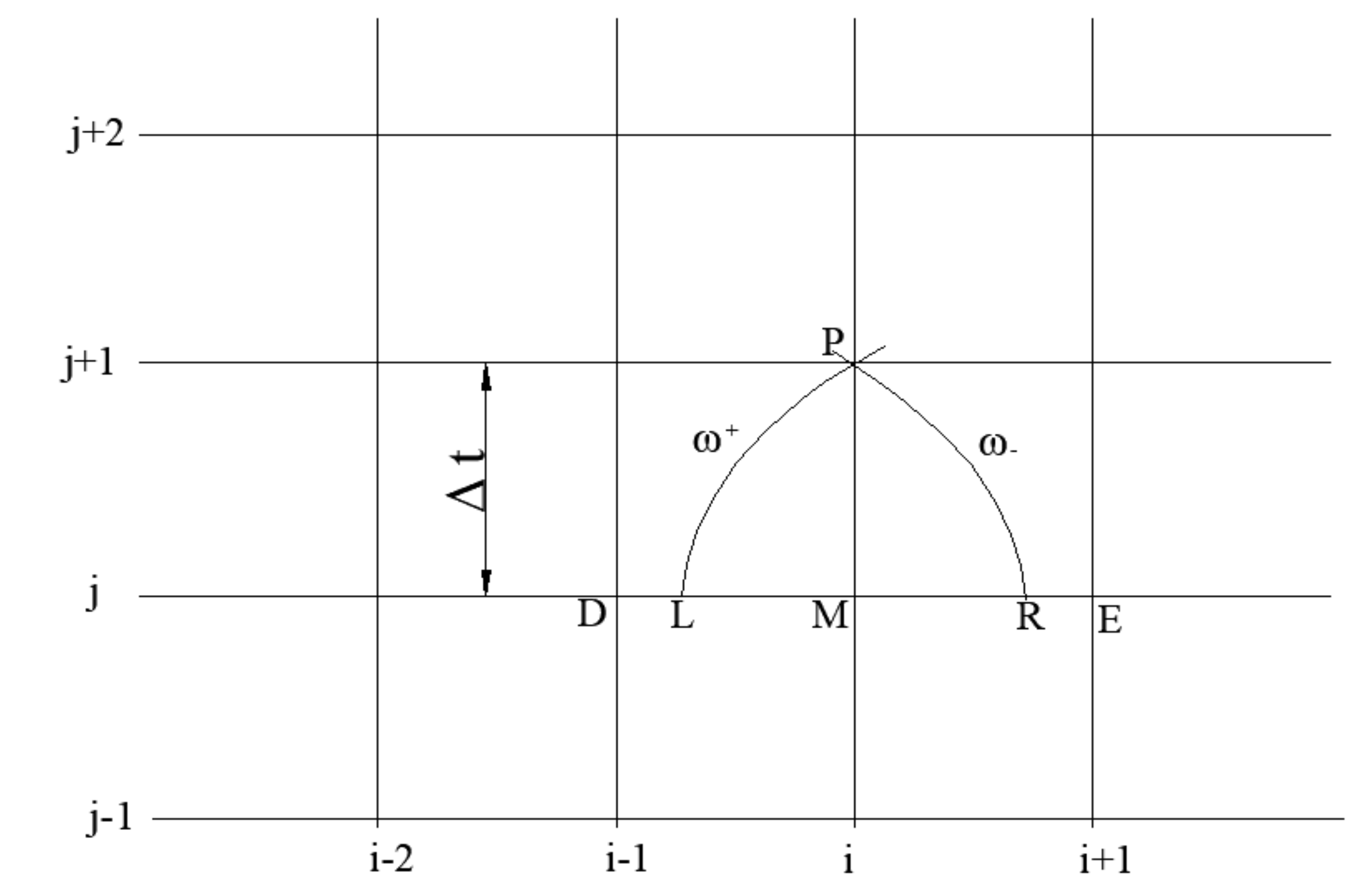
The rectangular grid feature difference method is used for discretization: first, the solution domain is divided into rectangle meshes according to time t and distance s. As shown in Figure 1, the intersection point of the mesh is called a node. Among them, i = 0, 1, 2, ..., n and denotes the segment number of distance s; j = 0, 1, 2, ..., n indicates the segment number of time t. $\Delta {\mathrm{s}}_{\mathrm{i}}={\mathrm{s}}_{\mathrm{i}}-{\mathrm{s}}_{\mathrm{i}-1}$ represents the distance step, that is, the length of the channel segment, which can be equal to the step size and variable step size; $\Delta {\mathrm{t}}_{\mathrm{j}}={\mathrm{t}}_{\mathrm{j}}-{\mathrm{t}}_{\mathrm{j}-1}$ indicates the time step, which needs to be determined based on the constraints of the stable format and the actual requirements. In Figure 1, the intersection point of the forward and backward characteristic lines (${\mathsf{\omega }}_{\pm }$) on the time layer j + 1 is the point P, and the intersection point with the time layer j is L and R, respectively. The node between them is M, and the left and right edges are points D and E, and the solution of the equation is to solve the hydraulic elements at the intersection P. When the initial conditions are given, the cycle calculation is solved according to the time step.

For solving the water level and discharge at point P, the points L and R need to be determined at first. These two points are not on the grid nodes and therefore the Courant’s scheme is used for linear interpolation. The integral theorem can be used to obtain the discrete results as follows:

$$\begin{array}{c}{\mathrm{Z}}_{\mathrm{L}}=\frac{\Delta \mathrm{t}}{\Delta {\mathrm{s}}_{\mathrm{i}}}{\left({\mathsf{\omega }}_{+}\right)}_{\mathrm{M}}\left({\mathrm{Z}}_{\mathrm{D}}-{\mathrm{Z}}_{\mathrm{M}}\right)+{\mathrm{Z}}_{\mathrm{M}}\\ {\mathrm{Q}}_{\mathrm{L}}=\frac{\Delta \mathrm{t}}{\Delta {\mathrm{s}}_{\mathrm{i}}}{\left({\mathsf{\omega }}_{+}\right)}_{\mathrm{M}}\left({\mathrm{Q}}_{\mathrm{D}}-{\mathrm{Q}}_{\mathrm{M}}\right)+{\mathrm{Q}}_{\mathrm{M}}\end{array}\}$$

(5)

$$\begin{array}{c}{\mathrm{Z}}_{\mathrm{R}}=\frac{\Delta \mathrm{t}}{\Delta {\mathrm{s}}_{\mathrm{i}+1}}{\left({\mathsf{\omega }}_{-}\right)}_{\mathrm{M}}\left({\mathrm{Z}}_{\mathrm{M}}-{\mathrm{Z}}_{\mathrm{E}}\right)+{\mathrm{Z}}_{\mathrm{M}}\\ {\mathrm{Q}}_{\mathrm{R}}=\frac{\Delta \mathrm{t}}{\Delta {\mathrm{s}}_{\mathrm{i}+1}}{\left({\mathsf{\omega }}_{-}\right)}_{\mathrm{M}}\left({\mathrm{Q}}_{\mathrm{M}}-{\mathrm{Q}}_{\mathrm{E}}\right)+{\mathrm{Q}}_{\mathrm{M}}\end{array}\}$$

(6)

$$\begin{array}{c}{\mathrm{Z}}_{\text{P}}=\frac{\left[{\left({\mathsf{\phi }}_{-}\right)}_{\text{M}}-{\left({\mathsf{\phi }}_{+}\right)}_{\text{M}}\right]\Delta \text{t}+{\left({\text{B}\mathsf{\omega }}_{-}\right)}_{\text{M}}{\mathrm{Z}}_{\text{L}}-{\left({\text{B}\mathsf{\omega }}_{+}\right)}_{\text{M}}{\mathrm{Z}}_{\text{R}}+{\mathrm{Q}}_{\text{R}}-{\mathrm{Q}}_{\text{L}}}{{\left({\text{B}\mathsf{\omega }}_{-}\right)}_{\text{M}}-{\left({\text{B}\mathsf{\omega }}_{+}\right)}_{\text{M}}}\\ {\mathrm{Q}}_{\text{P}}={\mathrm{Q}}_{\text{R}}+{\left({\text{B}\mathsf{\omega }}_{+}\right)}_{\text{M}}\left({\mathrm{Z}}_{\text{P}}-{\mathrm{Z}}_{\text{R}}\right)-{\left({\mathsf{\phi }}_{+}\right)}_{\text{M}}\Delta \text{t}\\ {\mathrm{Q}}_{\text{P}}={\mathrm{Q}}_{\text{L}}+{\left({\text{B}\mathsf{\omega }}_{-}\right)}_{\text{M}}\left({\mathrm{Z}}_{\text{P}}-{\mathrm{Z}}_{\text{L}}\right)-{\left({\mathsf{\phi }}_{-}\right)}_{\text{M}}\Delta \text{t}\end{array}\}$$

(7)

where $\mathrm{N}=\mathrm{B}{\left(\frac{\mathrm{Q}}{\mathrm{A}}\right)}^2\mathrm{i}-\frac{{\mathrm{gQ}}^2}{{\mathrm{AC}}^2\mathrm{R}}$, ${\mathsf{\phi }}_{\pm }=\left({\mathsf{\omega }}_{\pm }\right){\mathrm{q}}_{\mathrm{l}}-\mathrm{N}$.

At the same time, as the Courant’s scheme is a first-order explicit format, in order to make the calculation stable, it is necessary to choose reasonable distance and time steps to satisfy the condition of stability.

$$\frac{\Delta {\mathrm{s}}_{\mathrm{i}}}{\mathrm{v}+\sqrt{\mathrm{g}\frac{\mathrm{A}}{\mathrm{B}}}}\ge \Delta {\mathrm{t}}_{\mathrm{i}}$$

(8)

2.3. Boundary Conditions

The irrigation channel includes both internal and external boundary conditions. The internal boundary conditions refer to the changes in the boundaries of the gates and other control structures in the channel segment. The external boundary conditions refer to the inflow and outflow boundary conditions.

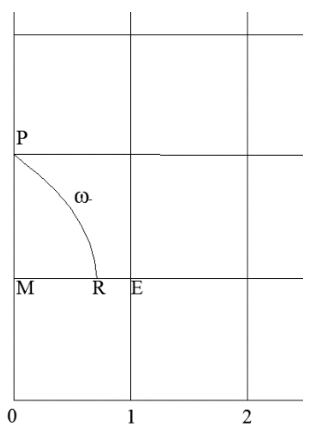
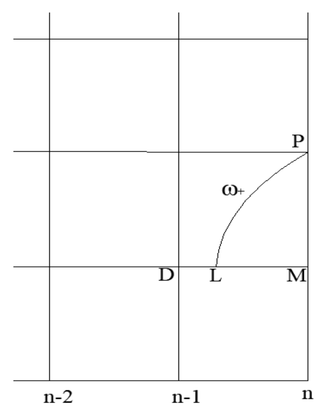
The above calculation format is only applicable to the calculation of interior points, as shown in Figure 2 and Figure 3. For the boundary points, there is only one characteristic line, and thus there are only two equations, but three unknowns, so it is necessary to supplement the boundary conditions. The following three conditions are common in the upstream and downstream boundary conditions:

(1)

Z = Z(t), i.e., the water level process is known;

(2)

Q = Q(t), i.e., the flow process is known; and

(3)

Q = f(Z), i.e., the relationship between the water level and the discharge is known.

2.4. Conditions at Branch Point

Since the irrigation channel is mostly tree-shaped there must be innumerous delivery in its layout. Irrigation channels are divided into four levels: dry, branch, bucket, and agriculture, which must be connected by a series of branches and exchange points. These connection points are branch points. At the branch point, the water flow must meet the corresponding connection conditions, i.e., discharge compatibility and energy compatibility conditions [19].

Discharge compatibility conditions:

$${\displaystyle \sum }_{\mathrm{i}=1}^{\mathrm{n}}{\mathrm{sl}}_{\mathrm{i}}·{\mathrm{Q}}_{\mathrm{i}}=0$$

(9)

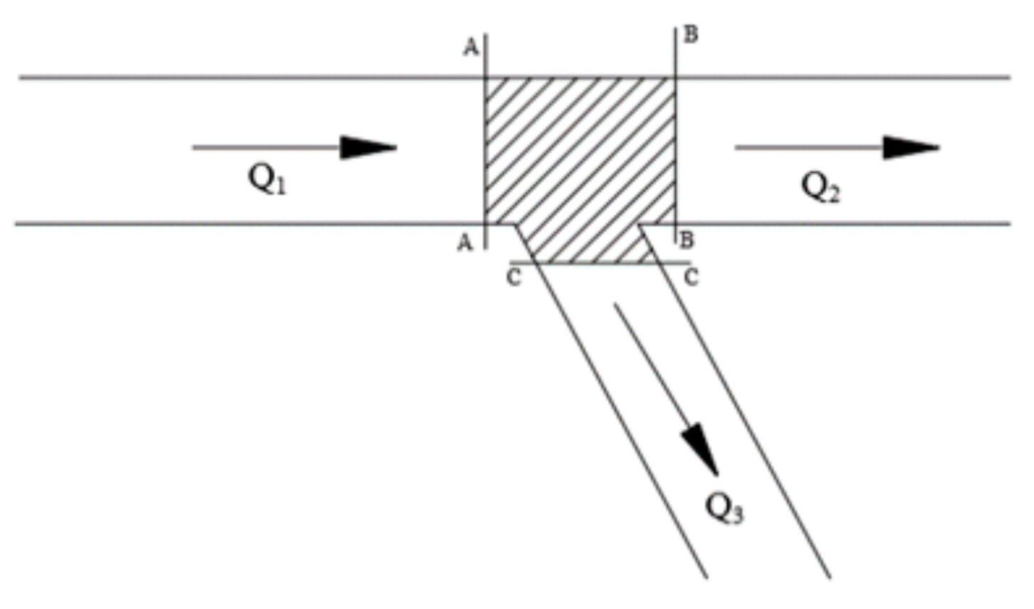
where n is the number of channels at the branch point; Q_i is the flow of the i-th channel at the branch point; When the channel water flows into the defect point ${\mathrm{sl}}_{\mathrm{i}}$ takes “+1”, and when it flows out, it takes “−1”. For the delivery channel as shown in Figure 4, the discharge compatibility condition can be written as follows:

$${\mathrm{Q}}_1={\mathrm{Q}}_2+{\mathrm{Q}}_3.$$

(10)

Energy compatibility conditions:

Firstly, the branch point is generalized to a geometric point. As shown in Figure 4, A-A, B-B, and C-C of the circle enclose a small drainage basin. Since only calculations are needed for the discharge or water level on the boundary section, the drainage basin may not be studied and the area of the basin is assumed to be zero. In an ideal situation, that is, no local head loss is considered, and there is no water level mutation in general. Therefore, there are:

$${\mathrm{Z}}_1={\mathrm{Z}}_2={\mathrm{Z}}_3$$

(11)

where ${\mathrm{Z}}_{\mathrm{i}}$ (i = 1, 2, 3) is the water level of the ith channel at the point. For irrigation channels, gates and other hydraulic structures are often found to be at the concrete sites. Therefore, considering the local head loss, the energy equations can be listed as follows:

$${\mathrm{Z}}_1+\frac{{\mathrm{v}}_1{}^2}{2\mathrm{g}}\left(1+{\mathsf{\alpha }}_1\right)={\mathrm{Z}}_2+\frac{{\mathrm{v}}_2{}^2}{2\mathrm{g}}\left(1+{\mathsf{\alpha }}_2\right)$$

(12)

$${\mathrm{Z}}_1+\frac{{\mathrm{v}}_1{}^2}{2\mathrm{g}}\left(1+{\mathsf{\alpha }}_1\right)={\mathrm{Z}}_3+\frac{{\mathrm{v}}_3{}^2}{2\mathrm{g}}\left(1+{\mathsf{\alpha }}_3\right)$$

(13)

where ${\mathsf{\alpha }}_{\mathrm{i}}$ (i = 1, 2, 3) is the energy correction factor and ${\mathsf{\alpha }}_1$ = 0.

3. Description of the Irrigation Channel System

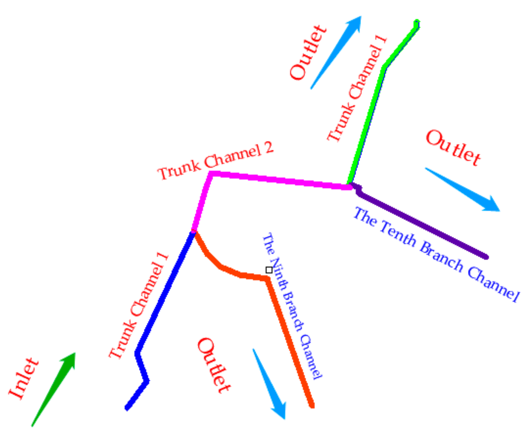
Yintang irrigation district is located in Tangyuan County, Heilongjiang province. The water source of the irrigation area is from Tangwang River. The designed irrigation area is 26,826 ha and the design discharge of total project is 160 m³/s. This study selected the north trunk channel, ninth branch and tenth branch as simulation regions. Each channel is a trapezoidal section and is lined with concrete. The layout of the channel is shown in Figure 5 and the relevant data are shown in

Table 1. Related channel information.

Channel’s Name	Total Length (m)	Base Width (m)	Bottom	Manning	Side Slopes of the Channel	Initial Flow (m3/s)
			Slope (i)	Coefficient (n)
Trunk Channel 1	2100	13	0.00007	0.0196	2	25.28
Trunk Channel 2	2700	13	0.00017	0.0200	2	25.28
Trunk Channel 3	2100	12	0.00014	0.0195	2	25.28
The Ninth Branch Channel	3000	1.5	0.00040	0.0180	1.5	1.02
The Tenth Branch Channel	2100	1	0.00050	0.0180	1.5	0.79

.

This study adopts the chase method for the simulation of the channel system, and solves each channel one by one. It uses the results from the simulation of the upper-level channel as the initial condition of the next-level channel. The bifurcation is based on the conditions of flow compatibility at the branch point, and the results of branch channel are subtracted from the result of dry channel as the initial condition of the next channel, so that the result is obtained step by step.

Simulation conditions: The total simulation duration is 200 min, and the time step value is calculated according to Equation (8): trunk channel 1, ∆t ≤ 62 s; trunk channel 2, ∆t ≤ 61 s; trunk channel 3; ∆t ≤ 62 s, the ninth branch channel, ∆t ≤ 108 s; and the tenth branch channel, ∆t ≤ 112 s. Therefore, the time step of simulation of each channel is taken as 60 s. All channels are operated in downstream with a constant water depth. The upstream flow of trunk channel 1 increased linearly from 25.28 to 30.11 m³/s in 20 min. The upstream flow of the ninth branch channel increased linearly from 1.02 to 1.32 m³/s in 20 min, and the upstream flow of the tenth branch channel increased linearly from 0.79 to 1.02 m³/s in 20 min. The downstream flow from the trunk channel 2 is reduced by the flow of the upstream section of the tenth branch channel, and a change in the flow of the upstream section of the trunk channel 3 is obtained.

4. Analysis of Simulation Results

Under the above conditions, the changes in the water level of the upstream section were simulated and the changes in the flow of the downstream section, and the obtained numerical results were used to compare with the simulation results obtained from MIKE11 to verify the reliability of the model.

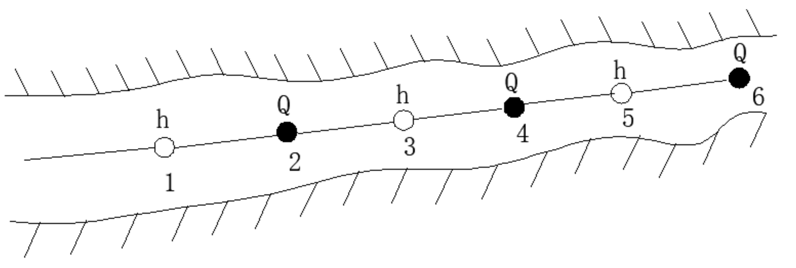
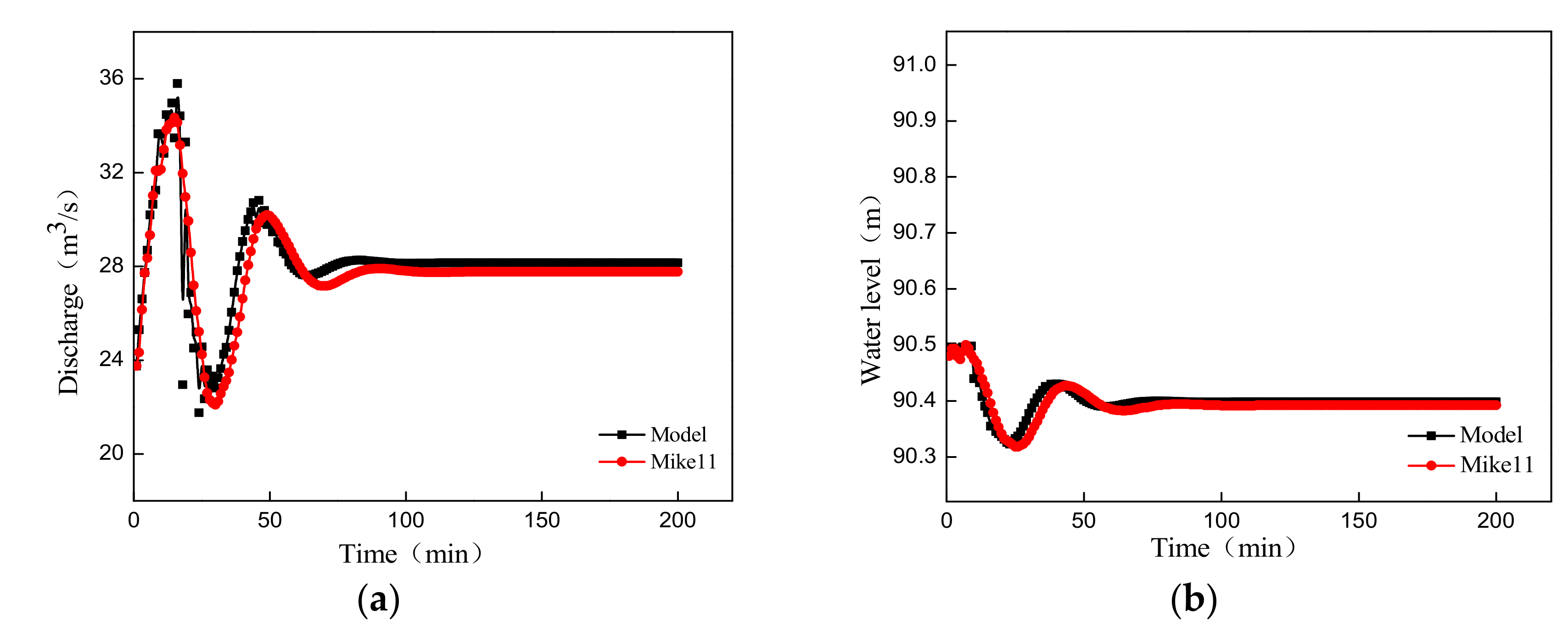
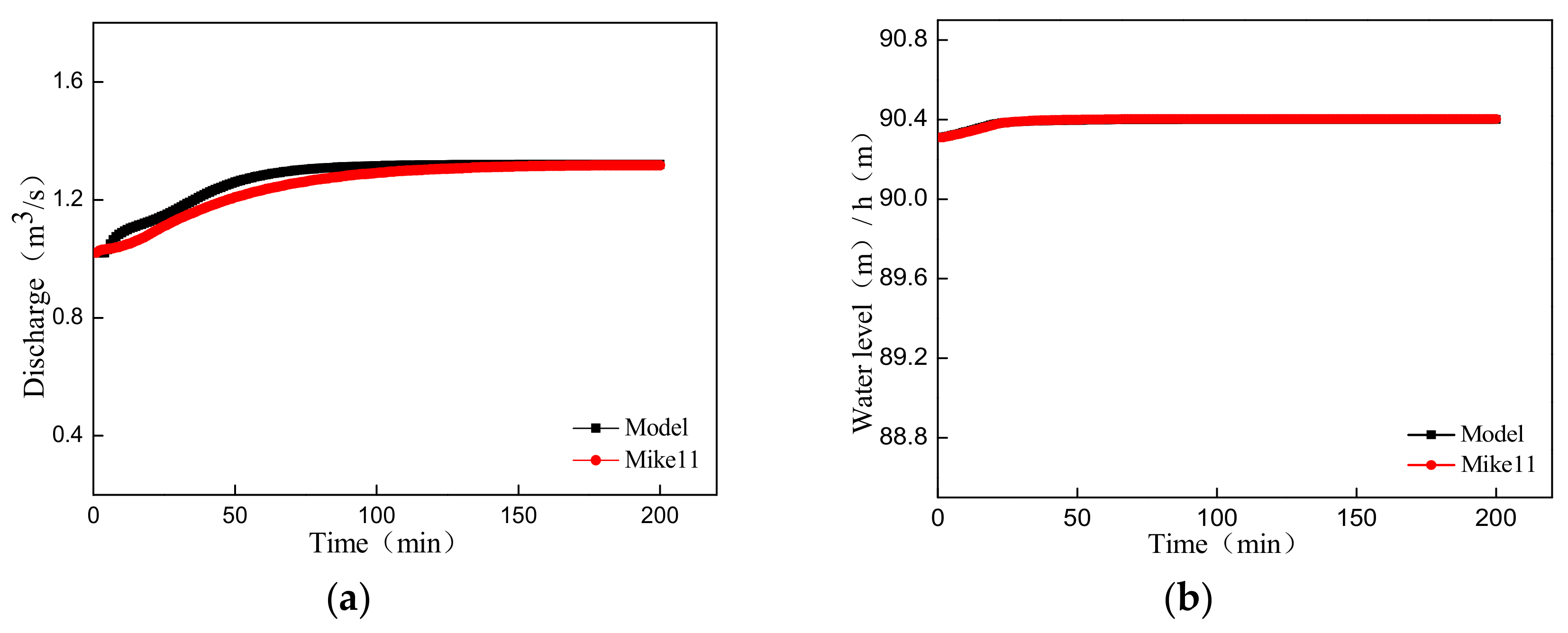
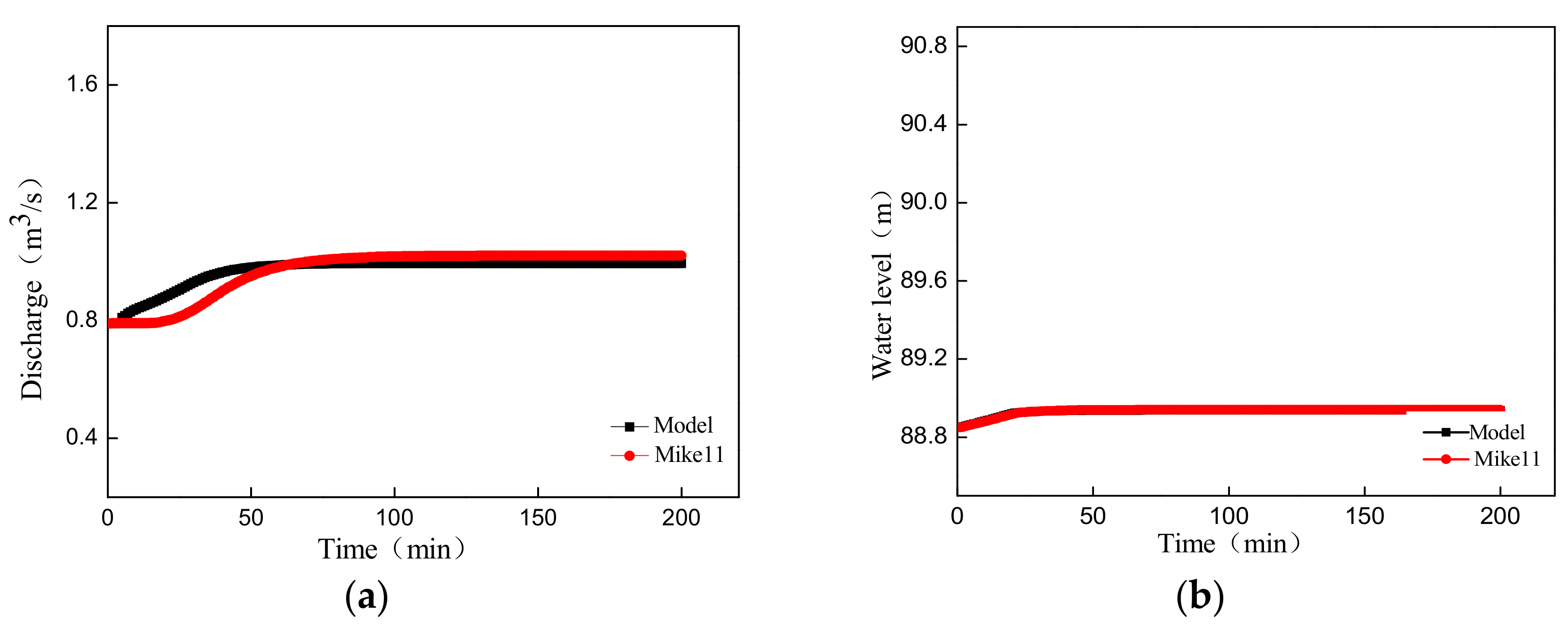
Where, MIKE11 model also uses the de Saint-Venant equations as the governing equations. In the model, the Abbott six-point implicit scheme is used to discretize the above control equations, and the water level and flow rate are alternatively calculated as h and Q points, respectively (Figure 6). The format is unconditionally stable and can be kept stable at a considerable Courant number, allowing for longer time steps to save the computation time. In addition, when using MIKE11 software for the construction of model, the third part of the text is used as the basis for making the cross-section and boundary files. The obtained simulation results are shown in Figure 7, Figure 8, Figure 9, Figure 10 and Figure 11 [20].

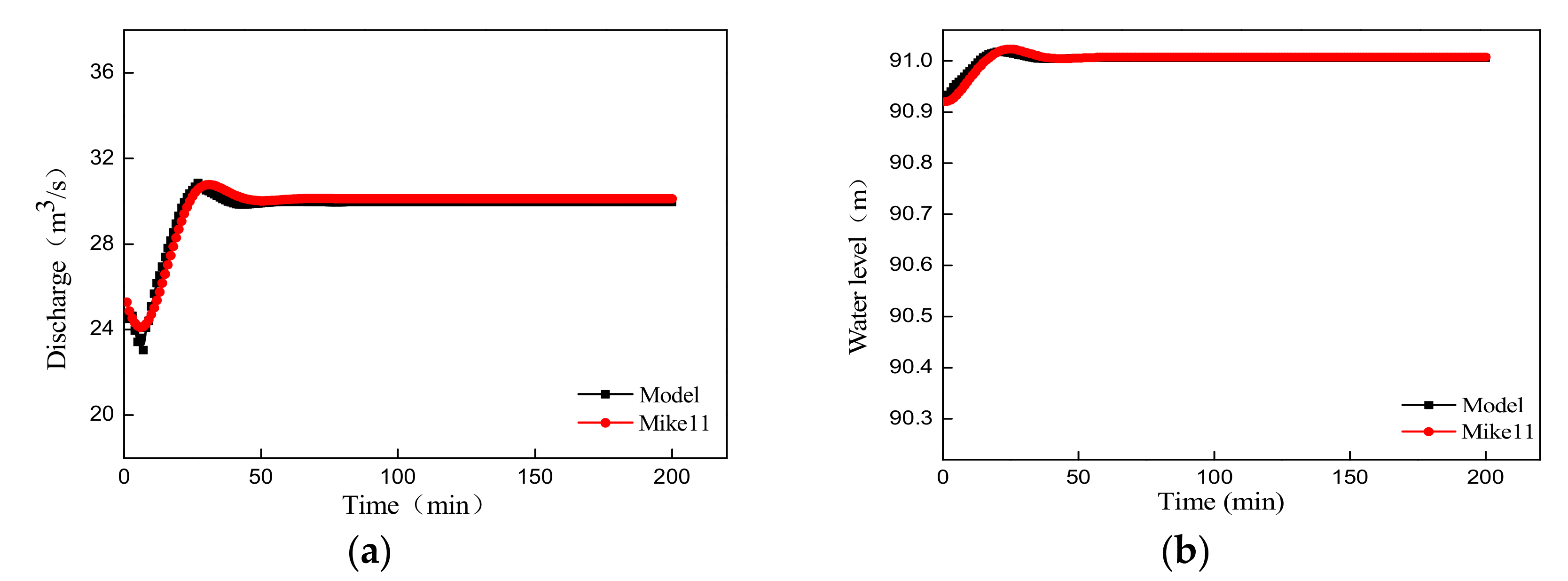
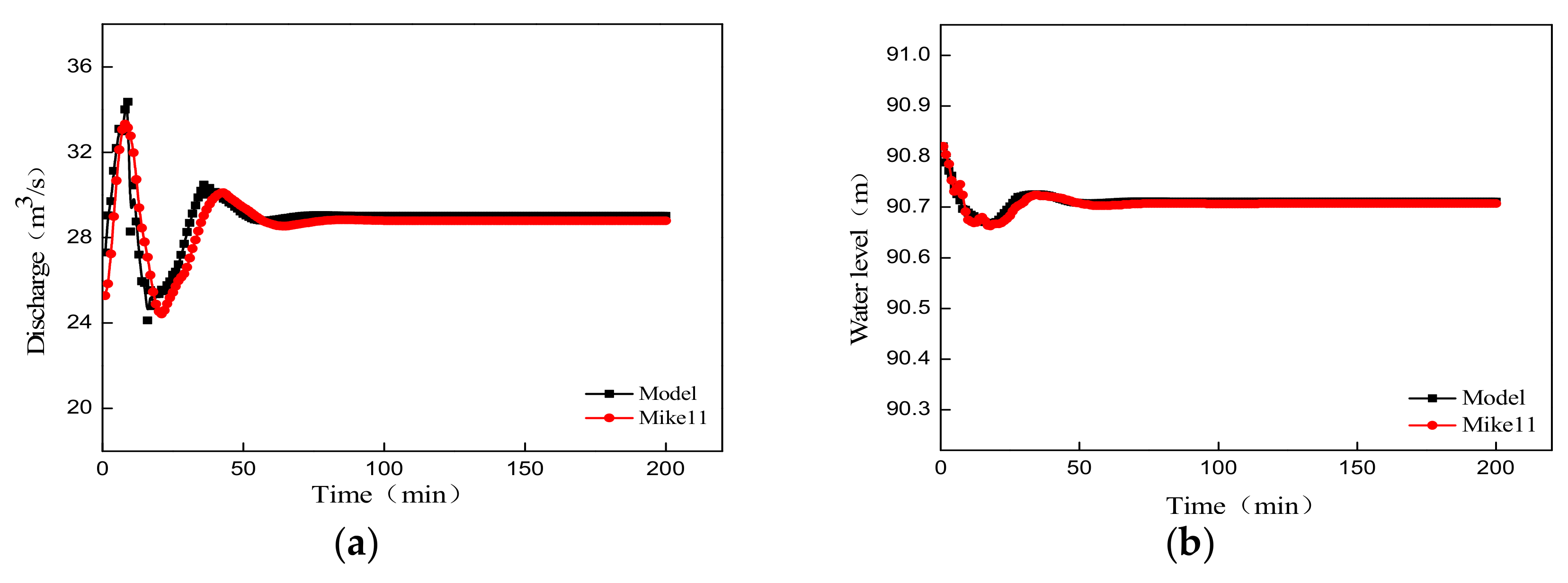
From the above simulation results, it can be seen that the model established in this study is satisfactorily consistent with the simulation results of MIKE11 model, even the two curves in Figure 10b and Figure 11b are roughly coincident, indicating that the simulation results of the model are very accurate. The obtained specific results are as follows:

(1)

When the upstream gates of trunk channel 1 were adjusted, the ninth and the tenth branch channels generated the corresponding flow according to the simulation conditions, and the water level and flow of each channel basically reached a stable level after 50 min.

(2)

The downstream flow of trunk channel 1 was stable after one fluctuation. Within 20 min of a linear increase in the flow, the upstream water level also showed a linear increase and after a small fluctuation it transformed to a stable state.

(3)

After the previous transmission and the diversion of ninth branch channel, the fluctuations in the downstream flow of the trunk channel 2 were more obvious. At the same time, the water level of the trunk channel 2 changed nonlinearly and stabilized after experiencing certain fluctuations. The regularity of the flow rate and water level of the trunk channel 3 were similar to that of the trunk channel 2, but after further propagation, the fluctuation was more obvious than the trunk channel 2.

(4)

Under the given conditions of simulation, the variations in the flow of the ninth branch channel was very small. Therefore, the downstream section had a small flow fluctuation which gradually stabilized. At the same time, when the flow rate increased linearly, the upstream water level also showed a linear increase, and then became stable. The changes in the flow and water level of the tenth branch channel were similar to the ninth branch channel, so we will not repeat them here.

5. Design of Gate Operation

5.1. Design of Gate Opening Adjustment

In irrigation channels, it is often necessary to adjust the gate according to the demand in the changes in the flow, which requires an understanding in the opening of gate over a given period of time. According to the channel model established in this study, the changes in the water level or flow corresponding to the gate section can be calculated, and the control process of the gate can be calculated based on the equation of the outflow of gate hole which provides the basis of decision-making for the staff.

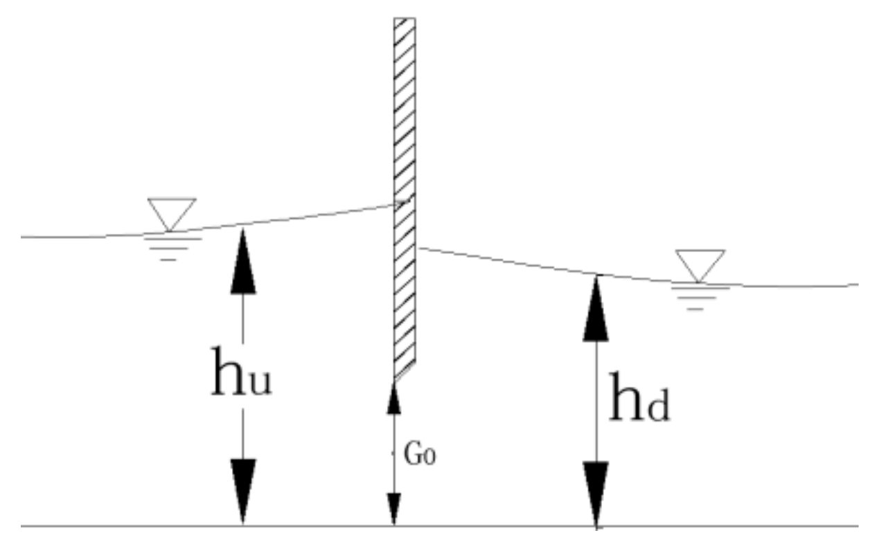
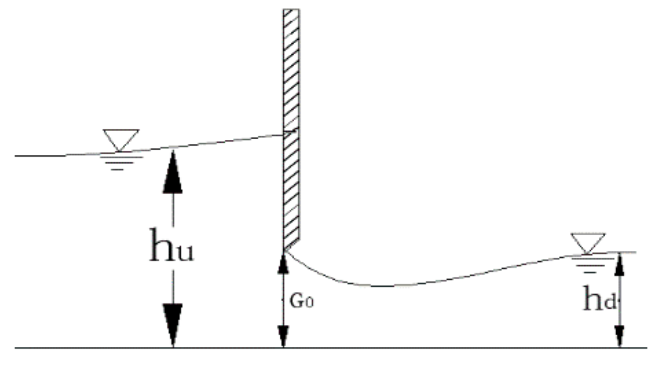
The sluice gate outflow can be divided into free and submerged outflows, as shown in Figure 12 and Figure 13 respectively. Their flow calculations have corresponding empirical equations which can be combined into the following formats [21].

$${\mathrm{Q}}_{\mathrm{z}}={\mathrm{c}}_{\mathrm{d}}\times {\mathrm{b}}_{\mathrm{z}}\times {\mathrm{G}}_{\mathrm{o}}\times \sqrt{2{\mathrm{gh}}_{\mathrm{u}}}$$

(14)

In the equation, Q_z represents the flow through the gate; b_z represents the gate width; Go represents the gate opening; h_u represents the gate upstream depth; and ${\mathrm{C}}_{\mathrm{d}}$ represents the discharge coefficient.

In 1950, Henry proposed a calculation method for the flab gate discharge coefficient under free-flow and submerged outflow through extensive experimental research, and plotted the curve of the sluice discharge coefficient [22]. Henry’s conclusion was later confirmed by Rajaratnam and Subramanya [23], and it is believed that different fitting curves for different outflow conditions are reliable. Hence, in 1992, Swamee fits the function according to the curve drawn by Henry [24], this function eliminates the cumbersome process of determining the flow coefficient by looking up the table, and is more conducive to programming calculation of the gate opening.

When ${\mathrm{h}}_{\mathrm{u}}\ge 0.81{\mathrm{h}}_{\mathrm{d}}{\left(\frac{{\mathrm{h}}_{\mathrm{d}}}{{\mathrm{G}}_{\mathrm{o}}}\right)}^{0.72}$, the gate shows a free flow:

$${\mathrm{C}}_{\mathrm{d}}=0.611·{\left(\frac{{\mathrm{h}}_{\mathrm{u}}-{\mathrm{G}}_{\mathrm{o}}}{{\mathrm{h}}_{\mathrm{u}}+15·{\mathrm{G}}_{\mathrm{o}}}\right)}^{0.072}.$$

(15)

When ${\mathrm{h}}_{\mathrm{d}}<{\mathrm{h}}_{\mathrm{u}}<0.81{\mathrm{h}}_{\mathrm{d}}{\left(\frac{{\mathrm{h}}_{\mathrm{d}}}{{\mathrm{G}}_{\mathrm{o}}}\right)}^{0.72}$, the gate shows a submerged flow:

$${\mathrm{C}}_{\mathrm{d}}=0.611·{\left(\frac{{\mathrm{h}}_{\mathrm{u}}-{\mathrm{G}}_{\mathrm{o}}}{{\mathrm{h}}_{\mathrm{u}}+15·{\mathrm{G}}_{\mathrm{o}}}\right)}^{0.072}{\left({\mathrm{h}}_{\mathrm{u}}-{\mathrm{h}}_{\mathrm{d}}\right)}^{0.7}·{\left\{0.32{\left[0.81{\mathrm{h}}_{\mathrm{d}}{\left(\frac{{\mathrm{h}}_{\mathrm{d}}}{{\mathrm{G}}_{\mathrm{o}}}\right)}^{0.72}-{\mathrm{h}}_{\mathrm{u}}\right]}^{0.7}+{\left({\mathrm{h}}_{\mathrm{u}}-{\mathrm{h}}_{\mathrm{d}}\right)}^{0.7}\right\}}^{-1}.$$

(16)

In the formula: ${\mathrm{h}}_{\mathrm{d}}$ represents the downstream depth of the gate.

In this model, the channel adopts the constant downstream water depth operation mode, and the flow rate of upstream changes linearly. Therefore, according to the flow of the cross section of upstream and the process of changes in the water level, the adjustment process of the degree of gate opening with time is deduced.

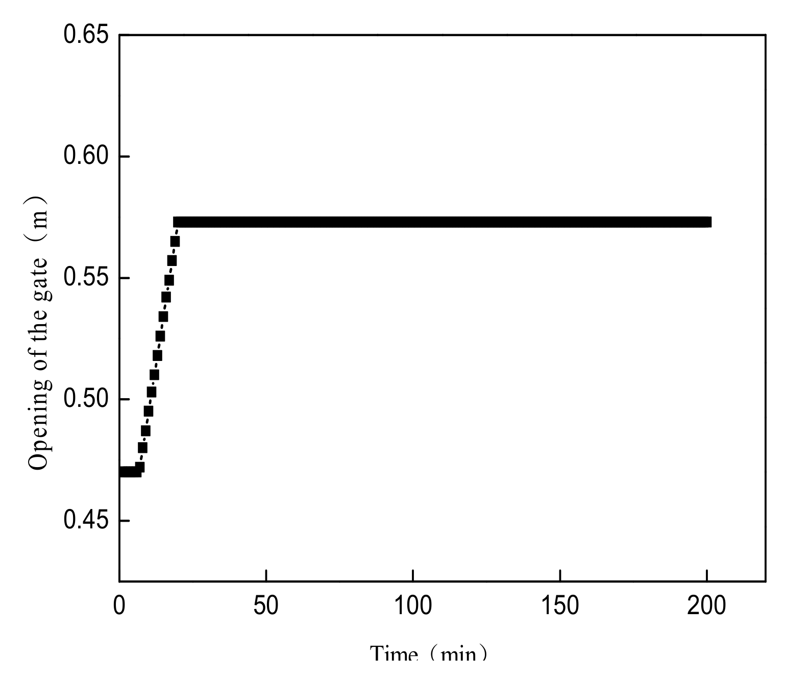
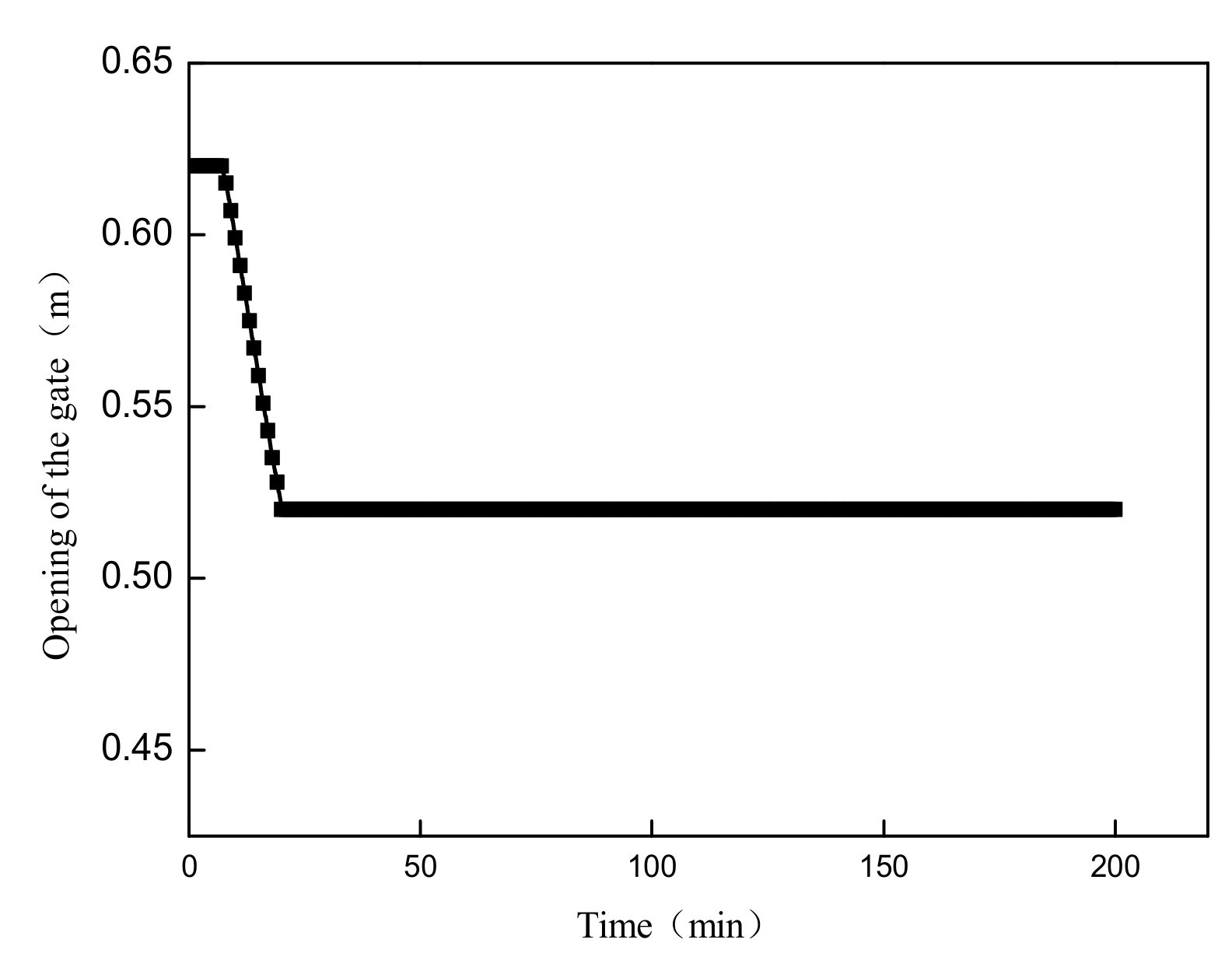
For the ninth branch channel, at first, the initial gate opening was obtained by trial calculations, where the water depth before and after the gate is seen to be 1.39 m and 0.66 m, respectively, whereas the width of the gate is 0.8 m. To start with gate opening was assumed, and then whether it belongs to free flow or submerged flow was judged, following which the discharge coefficient according to the corresponding equation was calculated, and finally by substituting in the Equation (14) the flow was found out and a comparison was made with the known initial flow. The trials were continued until they were consistent. By calculation, the initial gate opening of the ninth branch channel is 0.47 m. After obtaining the initial gate opening and using this as a starting point, the above process of trial calculation was used to solve the upstream section at every moment, and the adjustment process of gate opening at the upstream of the ninth branch channel can be obtained, as shown in Figure 14. As can be seen from this figure, the gate opening does not change within the first 5 min, which then increases linearly within 20 min and then remains unchanged. Also in this study, the changes in the opening of the gate when the flow rate was reduced from 1.32 to 1.02 was simulated, as shown in Figure 15. It can be noted from this figure that the opening of the gate remains unchanged within the first 7 min, which then increases linearly until reaching stability at 20 min.

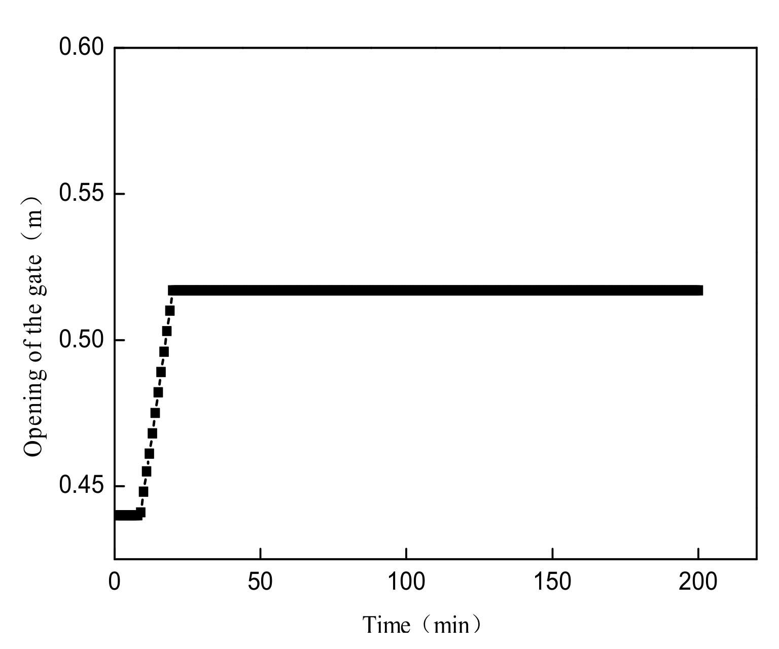
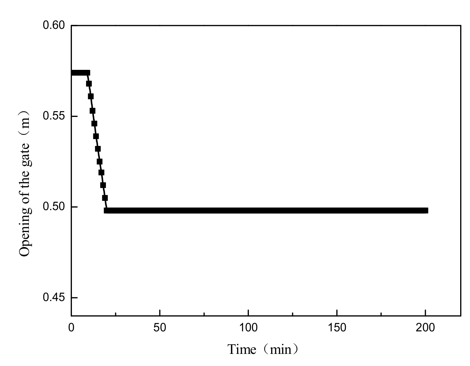
Similarly, the process of changing the gate opening when the flow rate of the tenth channel changed from 0.79 to 1.02 was simulated. The water depth before and after the gate is known to be 2.49 m and 0.63 m, respectively, and the width of the gate is 0.47 m. Through trial calculation, the opening of the initial gate is 0.44 m, and the regulation process is shown in Figure 16. As can be seen from this figure, the opening of the gate remains unchanged within the first 7 min, which then increased linearly until reaching stability at 20 min. When the flow rate changed from 1.02 to 0.79, the changes observed in the gate opening are shown in Figure 17. As can be seen from this figure, the opening of the gate remains unchanged within the first 9 min, which then increased linearly until reaching stability at 20 min.

5.2. Design of Multistage Gate Operation

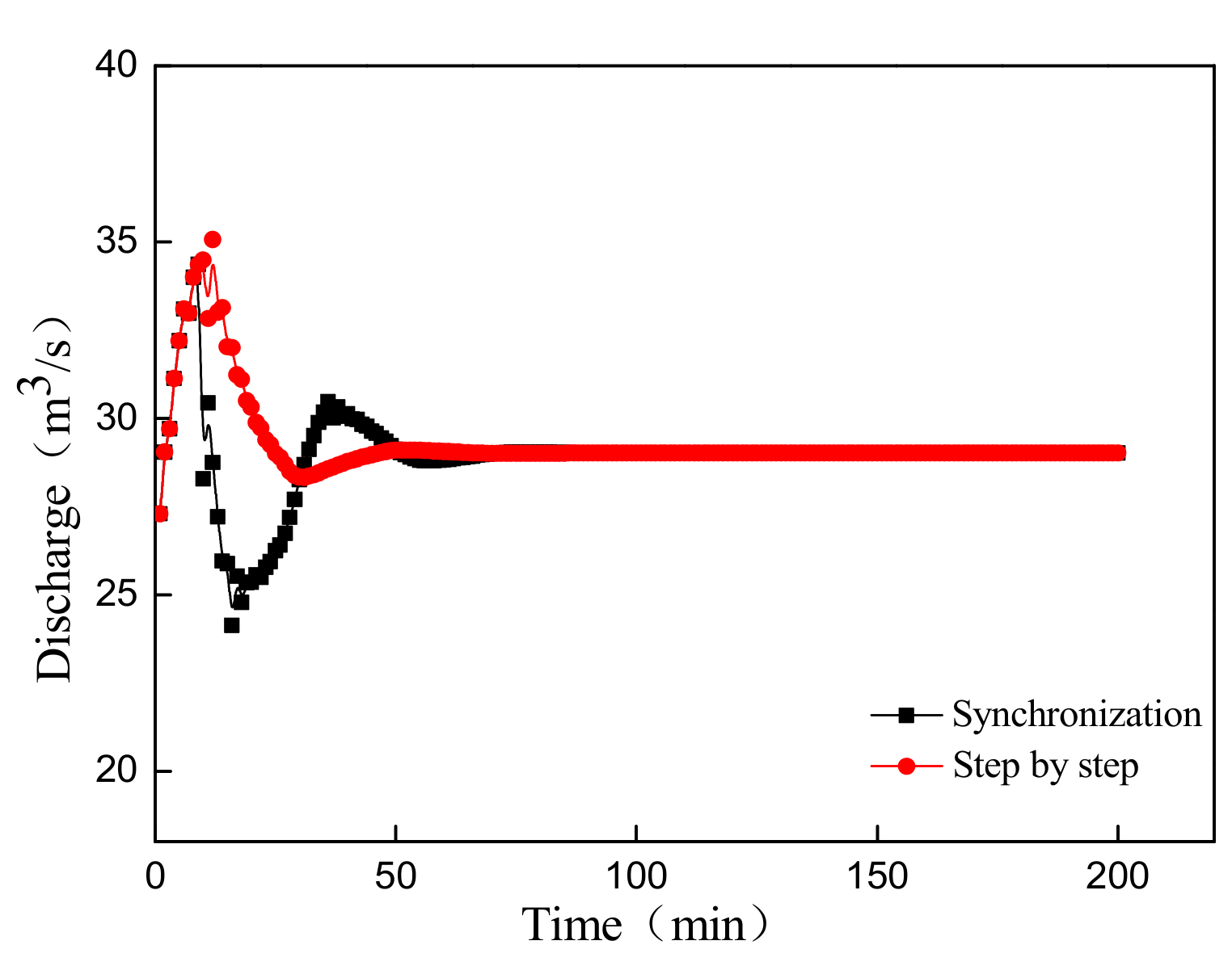
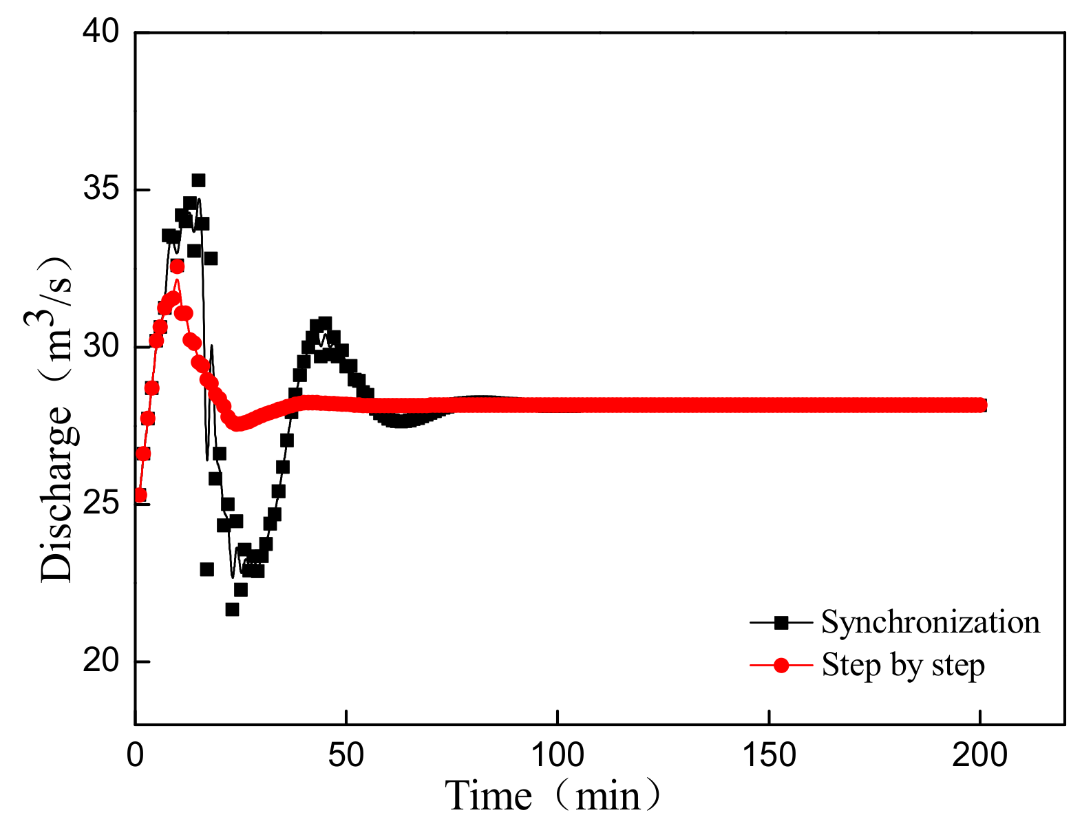
In the channel system, there are often multi-staged gates. When the gates are to be controlled to meet the requirements of the downstream flow, the gates at all levels can be adjusted at the same time, as well as they can be adjusted at a level one by one. In this way, the flow dynamics in the channel will be different under two modes of synchronization and step by step. In the above model, the simulation was carried out to simultaneously adjust the upstream gates of trunk channel 1, the ninth branch channel and the tenth branch channel. On this basis, the gradual adjustment was simulated, and after the trunk channel 1 reached a stable state, the gates of the ninth branch channel were adjusted, whereas after the trunk channel 2 was stabilized, the gates of the tenth branch channel were adjusted. Since the simulated conditions of the trunk channel 1, the ninth branch channel and the tenth branch channel were not changed, the changes in the flow of the trunk channels 2 and 3 were compared, as shown in Figure 18 and Figure 19.

From the above two figures, we can see that when the gates at all levels are synchronously adjusted, the fluctuations of water flow in the channel are continuously spread out and the range of fluctuation of the channels at all levels is more obvious. Also, the time of stability of each channel section is approximately the same, where they all stabilized after 50–60 min. The last level, that is, the north trunk channel 3, stabilized after 60 min. When the gates at all levels are adjusted step by step, the next gate is adjusted after the water flow in the upper-level channel reaches a stable level. Therefore, the fluctuations of the water flow in the channel cannot be propagated step by step. For all the levels of channels, the range of fluctuation is relatively small and the stabilization time is relatively short, where the stability reached after 35–40 min. However, in this case, it is not appropriate to only look at this channel, but should be started with the regulation of the upstream first-level gates. Therefore, the time for the fluctuations of water flow in the channel system to stabilize is 40 min of the north main channel 3 combined with the stabilization time of the upper-level channels, and the final total settling time is longer than under the synchronous control.

At present, most of the irrigation districts in China are unable to achieve synchronous control. In general, a step by step control is adopted, that is, first adjusting the gate head of the channel, and after the water flow in the channel reaches a stable level, and then the adjustment of the lower gate is performed. In this case, the fluctuations of water flow in the channel is small, the erosion of the channel is also smaller, the operation is more secure, the ultra-high standards of the channel can be reduced, and the overall project cost can be reduced. However, the operation is very complicated and the channel system takes longer to reach stability. If synchronous regulation is adopted, the total time taken for the channel system to reach final stability becomes short, and all levels of gates can be controlled at the same time, which is not based on the transition process of the upstream channels. The operation of gate opening and closing is simple and convenient, but in this case, the water flow in the channel is relatively large, which can scour the channel. In the actual irrigation process, if time is not a constraint, it is recommended to use a step-by-step regulation method; however, if it is necessary to meet the demand in a short period of time, then adopting a synchronous regulation method is recommended.

6. Conclusions

In this study, the specific process of discretization of de Saint-Venant system of equations by using the method of characteristics, the boundary conditions, bifurcation conditions, as well as the stability conditions employed in the model have been elaborated and the obtained results are as follows:

(1)

MIKE11 has a good simulation effect, but it cannot simulate the process of regulation of gate opening, besides being very costly. This study establishes a channel simulation model based on the method of characteristics, and simulates the transition process of the unsteady flows generated in the channels of the field. A comparison of the changes in the water level and flow rate simulated by the model with the simulation results of MIKE11 shows that the final results are very consistent, which proves that the model built in this study is very reliable.

(2)

Based on the simulation results of the model, a corresponding gate control model has been established. The observed results show that the changes in the gate opening are linear under the conditions of a linear increase or decrease in the flow. Also, the degree of adjustment of gate opening process of the ninth and the tenth branches can be obtained through calculations, and the fitted gate control equations are obtained which could be used as the basis for decision-making process for the relevant staff and also provides a basis for intelligent control.

(3)

The obtained results also show that under the conditions of synchronous control, the total regulation time is short and the gate opening and closing operation is convenient, however, the water flow in the channel fluctuates greatly. With a gradual control, the current fluctuations will be relatively small and the stability time will be shorter for each part of the channel, but in this case, the opening and closing of the gate is complex, and the total time of regulation will be longer. Therefore, if time permits a gradual control can be used.

In practice, the irrigation channel system of an irrigation area includes a trunk channel, a branch channel, a ditch and a farm channel, and notably its connection is very complicated. Therefore, on the basis of a simple simulation of the channel system, further extending to the simulation of more complex large-scale irrigation channels is still an important direction to be considered for future work. At the same time, due to the lack of measured data, this study fails to compare the simulation results with the measured data. Moreover, the model built in this study does not consider losses through channel leakage. The simulation of large bottom slope drop in the channel segment will also be distorted. These problems need to be constantly considered in the future work, which could continuously improve the model.

References

- Sun, J.; Kang, S. Present Situation of Water Resources Usage and Developing Countermeasures of Water-Saving Irrigation in China. Trans. CSAE 2000, 16, 1–5. [Google Scholar]
- Ministry of Water Resources the People’s Republic of China. China Water Resources Bulletin; China Water & Power Press: Beijing, China, 2016.
- Stoker, J.J. Report I. Numerical Solution of Flood Prediction and River Regulation Problems: Derivation of Basic Theory and Formulation of Numerical Methods of Attack; Report No. IMM-NYU-200; New York University Institute of Mathematical Science: New York, NY, USA, 1953. [Google Scholar]
- Isaacson, E.; Stoker, J.J.; Troesch, A. Report III. Numerical Solution of Flood Prediction and River Regulation Problems; Report No. IMM-NYU-235; New York University Institute of Mathematical Science: New York, NY, USA, 1956. [Google Scholar]
- Cooley, R.L.; Moin, S.A. Finite element solution of de Saint-Venant equations. J. Hydraul. Div. 1976, 102, 759–775. [Google Scholar]
- Holly, F.M., Jr.; Parrish, J.B., III. Description and evaluation of program: CARIMA. J. Irrig. Drain. Eng. 1993, 119, 703–713. [Google Scholar] [CrossRef]
- Schuurmans, W. Description and evaluation of program MODIS. J. Irrig. Drain. Eng. 1993, 119, 735–742. [Google Scholar] [CrossRef]
- Clemmens, A.J.; Holly, F.M., Jr.; Schuurmans, W. Description and evaluation of program: DUFLOW. J. Irrig. Drain. Eng. 1993, 119, 724–734. [Google Scholar] [CrossRef]
- Merkley, G.P.; Rogers, D.C. Description and evaluation program Canal. J. Irrig. Drain. Eng. 1993, 119, 714–723. [Google Scholar] [CrossRef]
- Han, Y. Study and Application of Irrigation Canal Based on Unsteady Hydraulic Modeling. Master’s Thesis, Northwest A&F University, Yangling, China, 2010. [Google Scholar]
- Wang, C.; Ke, S.; Feng, X. Using P+PR controller into Bival control algorithm for automatic operation of open channel. J. Wuhan Univ. Hydraul. Electr. Eng. 2000, 33, 11–15. [Google Scholar]
- Zhao, J.; Lu, W.; Zhao, L. Development of computer simulation technology for irrigation canal system. China Rural Water Hydropower 2001, 42, 9–12. [Google Scholar]
- Han, Y.; Lv, H.; Yu, G. Numerical Simulation of Unsteady Flow in Irrigation Canals with Two Operating Models. J. Yangtze River Sci. Res. Inst. 2010, 27, 29–33. [Google Scholar]
- Zhang, S.; Liu, Q.; Bai, M. Unsteady Water Flow Numerical Model for Irrigation Final Canal System Based on Scalar Finite-volume Method. J. Irrig. Drain. 2013, 32, 1–5. [Google Scholar]
- Xu, X.; Zhang, J.; Ding, J. Relaxation Iterative Method of Numerical Simulation for River Network Hydraulics and Water Surface Elevation Visualization. Hydrology 2000, 20, 1–3. [Google Scholar]
- Ma, H. Development of graphic display system for large-scale river networks and its application. J. Hohai Univ. (Nat. Sci.) 2002, 30, 107–110. [Google Scholar]
- Chen, D. Study on Visualization of Numerical Simulation for Unsteady Flow in River Networks. Master’s Thesis, Yangzhou University, Yangzhou, China, 2008. [Google Scholar]
- Lv, H.; Pei, G.; Yang, L. Hydraulics, 2nd ed.; China Agriculture Press: Beijing, China, 2011; ISBN 978-7-109-16474-1. [Google Scholar]
- Gu, Y.; Wang, S.; Guo, C. The calculation of unsteady flow with cross tributary in open channel. J. Tianjin Univ. (Sci. Technol.) 1985, 30, 54–64. [Google Scholar]
- Zhou, X.; Huang, L.; Wang, S. Application of MIKE 11 model in river network simulation of Nantong Plain. Jiangsu Water Resour. 2016, 19, 52–60. [Google Scholar]
- Yu, G. Numerical Simulation of Sluice Gate Regulated Unsteady Flow in Irrigation Canals. Master’s Thesis, Northwest A&F University, Yangling, China, 2004. [Google Scholar]
- Doulgeris, C.; Georgiou, P.; Papadimos, D.; Papamichail, D. Ecosystem approach to water resources management using the MIKE 11 modeling system in the Strymonas River and Lake Kerkini. J. Environ. Manag. 2012, 94, 132–143. [Google Scholar] [CrossRef] [PubMed]
- Rajaratnam, N.; Subramanya, K. Flow equation for the sluice gate. J. Irrig. Drain. Div. 1967, 93, 167–186. [Google Scholar]
- Swamee, P.K. Sluice Gate Discharge Equations. J. Irrig. Drain. Eng. 1992, 118, 56–60. [Google Scholar] [CrossRef]
Figure 1.
Schematic diagram of rectangular grid.
Figure 2.
Upstream boundary point.
Figure 3.
Downstream boundary point.
Figure 4.
Delivery channel.
Figure 5.
The layout of the channel.
Figure 6.
Alternate layout of water level point and flow point.
Figure 7.
(a) The change of the discharge in the (b). The change of the water level in downstream section of trunk channel 1 the upper section of trunk channel 1.
Figure 8.
(a) The change of the discharge in the (b). The change of the water level in downstream section of trunk channel 2 the upper section of trunk channel 2.
Figure 9.
(a) The change of the discharge in the (b). The change of the water level in downstream section of trunk channel 3 the upper section of trunk channel 3.
Figure 10.
(a) The change of the discharge in the (b). The change of the water level in downstream section of the ninth branch channel the upper section of the ninth branch channel.
Figure 11.
(a) The change of the discharge in the (b). The change of the water level in downstream section of the tenth branch channel the upper section of the tenth branch channel.
Figure 12.
Water level before and after the gate in free flow.
Figure 13.
Water level before and after the gate in submerged flow.
Figure 14.
Regulating process of the gate on the ninth branch channel when the flow rate increases.
Figure 15.
Regulating process of the gate on the ninth branch channel when the flow rate decreases.
Figure 16.
Regulating process of the gate on the tenth branch channel when the flow rate increases.
Figure 17.
Regulating process of the gate on the tenth branch channel when the flow rate decreases.
Figure 18.
Comparison of flow changes in the downstream of trunk channel 2.
Figure 19.
Comparison of flow changes in the downstream of trunk channel 3.