Estimating the Infiltration Area for Concentrated Stormwater Spreading over Grassed and Other Slopes


1
Department of Biosystems Engineering and Soil Science, University of Tennessee, 2506 E.J., Knoxville, TN 37996, USA
2
Efficient Energy of Tennessee, 7317 Clinton Hwy, Powell, TN 37849, USA
*
Author to whom correspondence should be addressed.
Water 2018, 10(9), 1200; https://doi.org/10.3390/w10091200
Submission received: 2 August 2018
/
Revised: 21 August 2018
/
Accepted: 31 August 2018
/
Published: 6 September 2018
(This article belongs to the Special Issue Stormwater Quality: Modelling, Monitoring, Risk Assessment and Remidiation)
Abstract
:This research developed a new approach for calculating the area over which water spreads after being released from a confined conduit onto a sloped planar surface with defined roughness. In particular, the goal was to predict how stormwater would spread onto a sloped grass lawn after being discharged from a disconnected gutter downspout or through a parking lot curb cut. The need for this stems primarily from regulators increasingly requiring developers to infiltrate more of the runoff created by site development, but designers not having good tools for estimating the infiltration area associated with such “overflow” practices. The model is largely based on Manning’s equation applied at multiple cross-sectional areas of flow downslope, with additional modifications allowing the water to spread laterally. The model results were compared to laboratory experiments of water spreading across a roughened painted surface and two different artificial turfs. The new model predicted the wetting area with average absolute errors of 6.0% and 5.9% for a fine-bladed artificial turf and a coarse-bladed artificial turf, respectively. In addition, while validating the modeled flow spreading across a range of roughnesses, the model had an absolute error of 5.2% for a rough painted surface meant to represent unfinished concrete.
1. Introduction
Jurisdictions specified as Municipal Separate Stormwater Sewer Systems (MS4s) are increasingly promulgating stormwater regulations requiring that certain depths of rainfall be infiltrated on development sites (United State Environmental Protection Agency [1]). These stormwater control measures (SCMs) include rain gardens, green roofs, bioretention cells, subsurface infiltration galleries, and the like. For many types of new construction—particularly suburban domestic housing—an appealing option is to disconnect gutter downspouts such that the roof runoff is directed across a grass lawn for additional infiltration. This SCM may be particularly effective for the smaller storms usually targeted by regulations, generally 1 to 1.5-in. [2]. Similar benefit can be achieved for parking lot runoff by discharging the flow onto a grassy lawn through a curb cut.
Most of the stormwater manual SCM descriptions (e.g., Tennessee Stormwater Manual [3]) provide minimal guidance on what infiltration area can be claimed for a simple downspout or curb cut disconnect. If an engineered level spreader is installed to force sheet flow onto the grass, the infiltration area is clearly defined as the width of the spreader multiplied by the flow length, but what infiltration area will result from simply discharging a fairly energetic concentrated flow from a downspout or curb cut onto a planar lawn? A literature search found no simple method addressing this question directly. The studies most closely related appear to be in the area of mudflow spreading [4] and basin irrigation advance [5], but the boundary conditions, scale, and even dynamics are different.
Infiltration-based models such as the EPA Stormwater Calculator (EPA, [6]) and the Tennessee Runoff Reduction Assessment Tool [7] require knowledge of the stormwater measure’s wetted area in order to calculate infiltration, so using these to model a disconnect requires prior calculation of that wetted area. Once the wetted area is calculated, along with other parameters such as soil texture, infiltration can be calculated using empirical models such the modified Kostiakov–Lewis method [8,9,10] or more physically-based models such as Hydrus [11]. Even with just a simplistic understanding of overland water flow, the following behaviors are expected: (1) larger flowrates will wet a larger area, as they will initially be deeper and thus spread more; (2) shallower slopes will result in larger wetted areas, as the downslope velocity will be lower so the flow will have more chance to spread; (3) rougher surfaces will result in larger wetted areas, as the greater flow resistance will cause slower deeper flow and subsequently more spread; and (4) longer slopes will provide more distance for spreading so will result in larger wetted areas.
Approaches to define spreading such as for irrigation basins described in [5] emphasize the wave-like aspects of the wetting front, because advance time is a substantial portion of the total irrigation time. In contrast, for overflow SCMs the advance time is very short (perhaps seconds or at most minutes) while the total overflow time will be on the order of 6–24 h. In such a case, it seems reasonable to model the steady flow that will dominate during most of the event. Based on this and examination of multiple approaches that failed to adequately represent one or more of the four points listed above, it was decided to use Manning’s equation at multiple cross-sections along the slope to define downslope flow, coupled with an additional approach to define the rate of spreading between cross-sections. Through utilization of a Manning’s equation based approach, mass balance is assured.
In addition to these conclusions, it is also evident that when water discharges at relatively high velocity from a restricted conveyance onto an unrestricted planar slope, the high initial downslope momentum and zero initial lateral velocity cause the water to proceed downslope for some distance prior to achieving significant lateral velocity as the plume begins widening. Early lateral spreading is driven by the flow “falling” in the outward cross-slope (lateral) direction under the force of gravity, and there is initially little lateral frictional resistance as lateral velocities are minimal. After some short time, however, lateral velocities have increased sufficiently that the resulting resistance to lateral flow becomes significant, and lateral flow can also be modeled using Manning’s equation.
It is the goal of this study to develop and test a new model initially based on this lateral acceleration due to gravity and subsequently on Manning’s equation to calculate the areal spreading of initially confined flow discharging onto an unconfined sloped plane with a defined flow resistance. The model will then be validated against laboratory tests using a range of flow rates, slope grades, and roughnesses.
2. Methods
2.1. Model
The well-known Manning’s equation describes open channel flow by
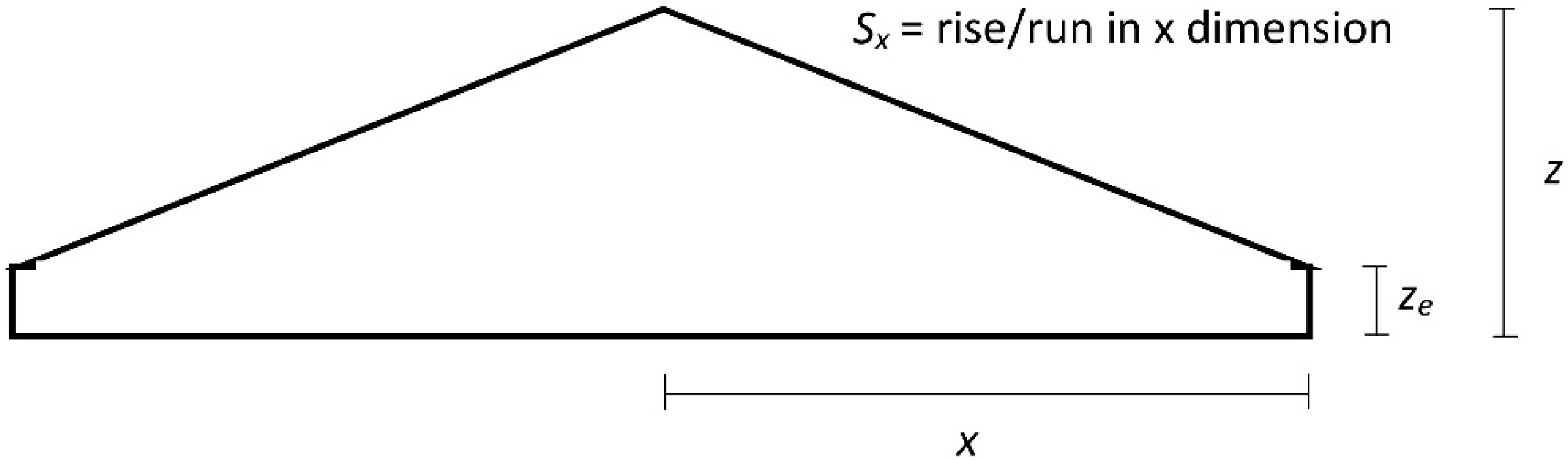
where Q is the volumetric flow rate, vy is the average water velocity downslope, A is the cross sectional flow area, k is a unit constant (1 for SI or 1.49 for US customary units), n is the Manning’s roughness coefficient, Rh is the hydraulic radius equal to A divided by the wetted perimeter, and Sy is the slope (rise/run) of the energy grade line which for this research is assumed to equal the bed slope (Manning [12]; discussed in detail in Chow, [13]). Unlike with most uses of Manning’s equation, for the current scenario the flow is on a planar surface without confining sides. Since Manning’s equation requires an estimate of the flow cross-section, it is assumed that as the water moves downslope, it maintains a triangular cross sectional set atop a small rectangular base with the dimensions labeled as shown in Figure 1. Other similar cross sections were investigated including an arc and various sections of ellipses in lieu of the triangular shape, but these shapes yielded no improvement over the simple cross section shown in Figure 1.
The overall approach is to assume symmetry and calculate the dimensions of x (half of wetted width) and z (maximum depth, occurring at the center edge of the half-section) as the water moves downslope. The downslope movement is assumed to be controlled by Manning’s equation, so it is calculated by applying Equation (1) at each narrowly-spaced cross-section. The lateral spreading that occurs as the plume moves downslope is dictated by Sx, the water surface slope in the cross-slope x-direction perpendicular to Sy. Initially this outward acceleration is driven solely by gravity, and its velocity (vx) is limited by the potential acceleration through time as the water starts to “fall” in the direction of Sx once the downspout sides no longer constrain lateral movement. Very quickly, however, vx becomes large enough to create its own frictional flow resistance such that pure response to gravity no longer accurately describes the acceleration in the x-direction. Following this point, the model switches to a different regime where the spreading is based on the ratio of Sy to Sx. This allows the water to flow in the direction of the vector sum of Sy to Sx without regard to further acceleration in the x-direction due to gravity.
In order to make the model as simple and usable as possible, the necessary user inputs are Q, Sy, n, k, and x0 = width of one half of the cross section just as the water exits the constraining downspout or curb cut; ze = the minimum water height at the edge of flow due to surface tension effects; ytarget = length of flow in the downslope direction, so the desired distance downslope over which the model should predict its spreading. In addition, the model assumes the initial velocity in the x direction at the inlet (vxo) is zero. Given the geometry in Figure 1, Equation (1) can then be rewritten as
At the first cross-section (just as the flow leaves the restraining inlet), the height of z is calculated iteratively from Equation (2) using the known Q, k, n, x0, ze, and Sy. From this point on, rather than looking at specific cross-sections spaced at some distance dy downslope, it is numerically simpler to conceptually “track” a single cross-section downslope in time, relying on the fact that dy = vy × dt. Then, in a similar fashion to what was done above at the first cross-section, vy and then y(i) can be calculated at each timestep utilizing the geometry in Figure 1 in concert with Equation (1) to yield
where dt is the timestep duration (initially set to 0.01 s), and (i) and (i−1) represent the current and previous timesteps, respectively.
The vy in this relationship describes the average cross section flow velocity downslope, but the velocity at the plume edge must also be known. By considering only an infinitely thin sliver of the cross section at its outer edge, the velocity in the y-dimension at this outer edge, (vy0) is calculated by reducing Equation (3) to
Sx is described at each step downslope by
which is utilized to determine the acceleration of water and ultimately vx, the velocity in the x-dimension. Assuming an initial vx0 = 0, the water rapidly accelerates in the x-direction due to gravitational forces described by Sx. The vx after each timestep in this “falling water” phase can be described via simple Newtonian physics as
where g is the acceleration due to gravity. Equation (7) is valid when the water is accelerating laterally due to gravitational forces only and is not greatly limited by flow resistance in the x-direction. Such a state ends quickly as vx increases, but incorporating an initial vx0 = 0 and letting it increase due to gravity-driven acceleration allows the water to shoot out of the conduit downslope in the direction of y for some distance prior to significant spreading in the x dimension. In other words, it serves to partially model the initially high downslope flow momentum.
After a short time, flow resistance to vx becomes significant, so it is necessary to provide a secondary means of modeling the lateral movement dependent on Manning’s equation. This was accomplished by calculating at each timestep the terms:
At the timestep following the point at which Sratio ≥ vratio, use of Equation (7) ceases, and vx is instead calculated as
which effectively sets vx proportional to vy in terms of their respective slopes. Once the change from use of Equation (7) to Equation (10) takes place, it is not allowed to return to a state using Equation (7), limiting the potential for numerical instability. The cumulative displacement in the x-dimension is calculated by
which allows for plotting all important results against elapsed time, t
The model continues until
which indicates that the wetted zone reaches the end of the target area.
Selection of a Manning’s n for use in Equation (1) is generally done by picking a value from a table of previously published values or simply fitting n to measured data. USDA-NRCS [14] suggests shallow-flow values of n = 0.24 for dense grasses and 0.41 for Bermuda grass, which are generally some of the highest values found in the tables. At the other end of the spectrum, for very shallow flows over paved surfaces Reed and Kibler [15] showed that n is directly related to S1/2. For example, if n = 0.013 (the table value for shallow flow over concrete) at a slope of 2.3%, then the n at a slope of 13.3% is calculated as follows
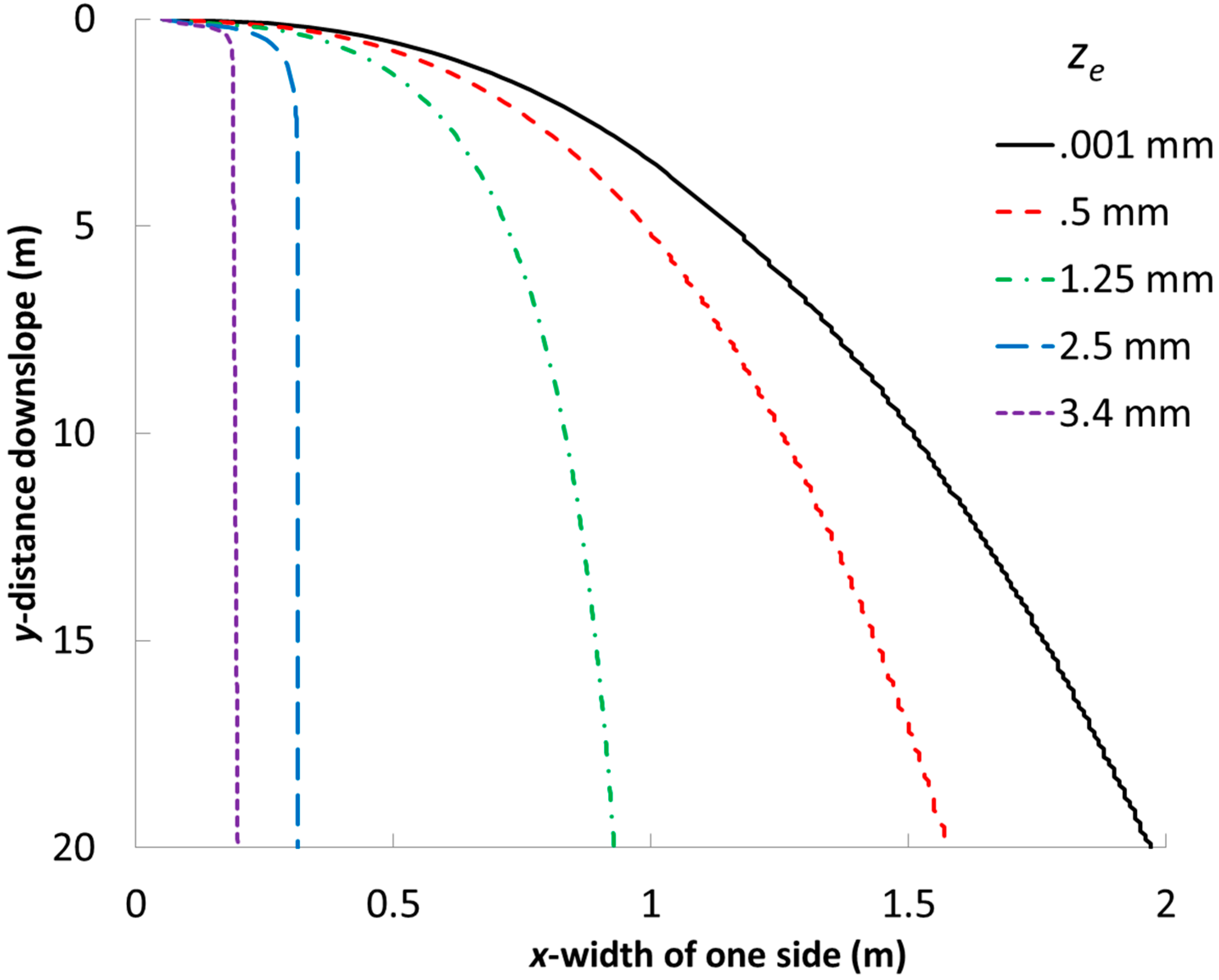
Selection of a value of ze for Equations (2), (3), (5) and (6) was not obvious, as there are not readily published values for this variable as there are for n. Clearly it must be between zero and some reasonable upper limit. If ze = 0, the flow plume will widen without limit as y increases. On the other hand, large values of ze limit the maximum width of the wetted path by reducing Sx. As z approaches ze when y becomes large, Sx approaches zero and no further increase in width is predicted. Simmons et al. [16] describe the depth of spilled fluids on dry concrete and found water puddles had a height of 3.4 mm on flat surfaces. They also describe how the height varies from thinner on upslope portions of puddles compared to downslope portions of puddles. Given the systems modeled—flow on potentially steep slopes, and on a very uneven texture—this study used ze as a fitting parameter limited between 0 and 3.4 mm. Mathematically, the impact of ze can be illustrated by setting z = ze, which reduces Equation (2) to
and shows that ze is inversely related to x.
2.2. Physical Testing
A 2.5 m × 2.5 m sloped wooden platform was constructed for testing. The slope of the platform was modified with jackstands located at its lower edge, and Sy was determined by measuring the height from the floor of the upper and lower edges of the platform along with the known platform dimensions. The top surface of the platform was coated with a latex paint with small amounts of medium sand mixed into it prior to application. This served the dual purposes of sealing the wood surface and slightly roughening the surface with the intent of approximating unfinished concrete. Though concrete will obviously never be used in an infiltration area, this surface is included in the tests to provide validation of the flow-spreading model across a very wide range of n values.
A hydrograph generator [17] in a constant flowrate mode supplied water to the platform. The actual flowrate delivered to the testing surfaces was measured volumetrically immediately prior to every test run, using a container of known volume and a stopwatch. This hydrograph generator is capable of delivering flow rates between 0.0114 LPM to 1440 LPM, easily providing the range of flows desired for this study. The hydrograph generator outflow was directed into a 10.2-cm wide (to reflect a 4-inch downspout) by 91.4 cm long aluminum trough fastened directly onto the platform to ensure it had the same Sy as the platform itself. With this configuration, water coming from the hydrographic generator exited the trough in an unrealistically energetic and turbulent manner, so an aluminum sheet with 0.635 cm hole perforations was placed just below the hydrograph generator output (1/4 the way down the length of the trough), such that turbulence was dampened somewhat prior to water exiting the trough onto the platform. When testing the artificial turfs, these were rolled out on the painted wood surface, and the trough was fastened on top of the turf.
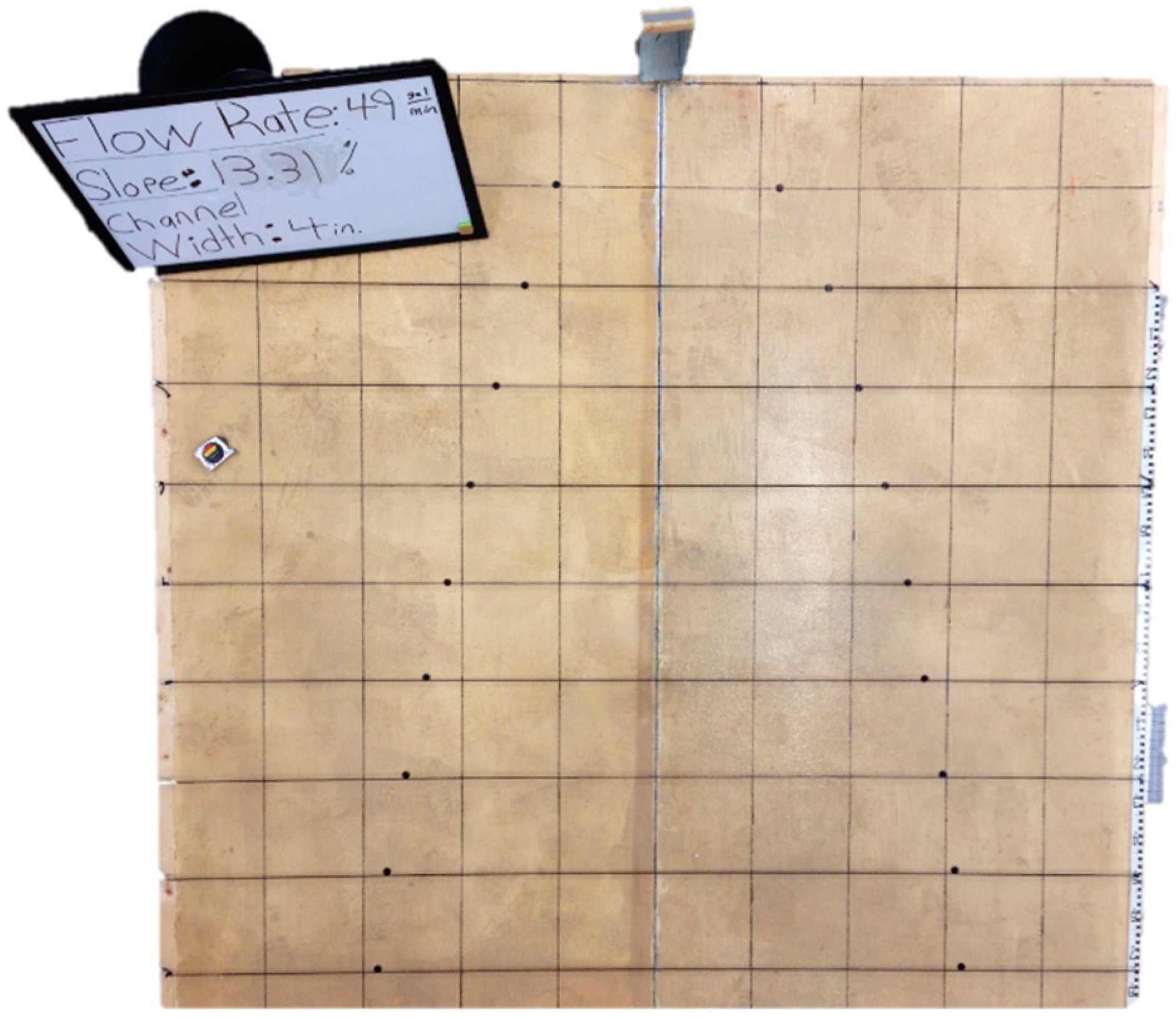
In order to quantify the spreading of the water plume, the platform was gridded into uniform 25 cm × 25 cm sections using thin black rope attached to metal eye hooks surrounding the perimeter of the platform. The rope grid was removed and reinstalled with every change of surface material. The rope was elevated approximately 5 cm above the platform such that it would not interfere with the water flow for any of the surfaces.
2.3. Testing Protocol
The sand roughened paint, fine-bladed artificial turf (4.45 cm pile height comparable to Greenline Classic 54™), and coarse artificial turf (5.1 cm pile height comparable to ProGreen Playground Extreme™) were tested to evaluate the areal spreading expected from water exiting a detached downspout onto a paved surface or a lawn. All three surfaces were exposed to multiple flowrates ranging from 45–185 LPM (12–49 GPM), and multiple slopes from 2.25–16.3%. If the discharges were from a roof with an area of 100 m2, the flowrates would correspond to precipitation rates of 2.7–11.1 cm/hr (1.1–4.4 in/hr). TSM (2015) suggests slopes up to 15% for Type A soils used as infiltration areas. Not every surface was extended to the highest flowrates, as for some combinations the 2.5 m × 2.5 m platform proved too small. For example, at the highest flow rates at the lower slopes the turf caused the flow to spread beyond the platform edges before it reached the bottom of the platform.
As each test began, water was allowed to flow over the testing surface until lateral spreading of the water had stopped and steady-state conditions were achieved. The time for this to occur depended on the flowrate, slope steepness, and surface cover, but generally ranged from about 20 s to a minute. Once the spreading stopped (but while flow continued), markers were placed by hand every 25 cm along the y-axis of the grid along both sides of the wetted perimeter (Figure 2). Photographs were taken from approximately 4 m above the center of the platform, allowing the entire testing surface to be captured on one image. The x-value for each marker was determined from the grids on the photographs, resulting in x-y coordinates for every 25–cm in the y dimension for both sides of the wetting front. An average measured x value was then calculated from the left and right side values of x for every value of y. This is the measured x value in all references below.
The fine and coarse artificial turfs used during testing were manufactured with small holes within the underlying sheet to allow water to drain through them. This was problematic because our test required that all of the water be kept flowing above the surface in order to contribute to spreading. Because the model requires a known Q, it was necessary to ensure that no water flowed through and underneath the turf such that any error in measuring the actual Q flowing atop the turf was minimized. To resolve this, waterproof caulk was used to seal the holes, then three coats of water resistant paint were applied to the backside of the turf. This was very effective, and visual observation during testing verified that there was no water leaking underneath the turf.
3. Results
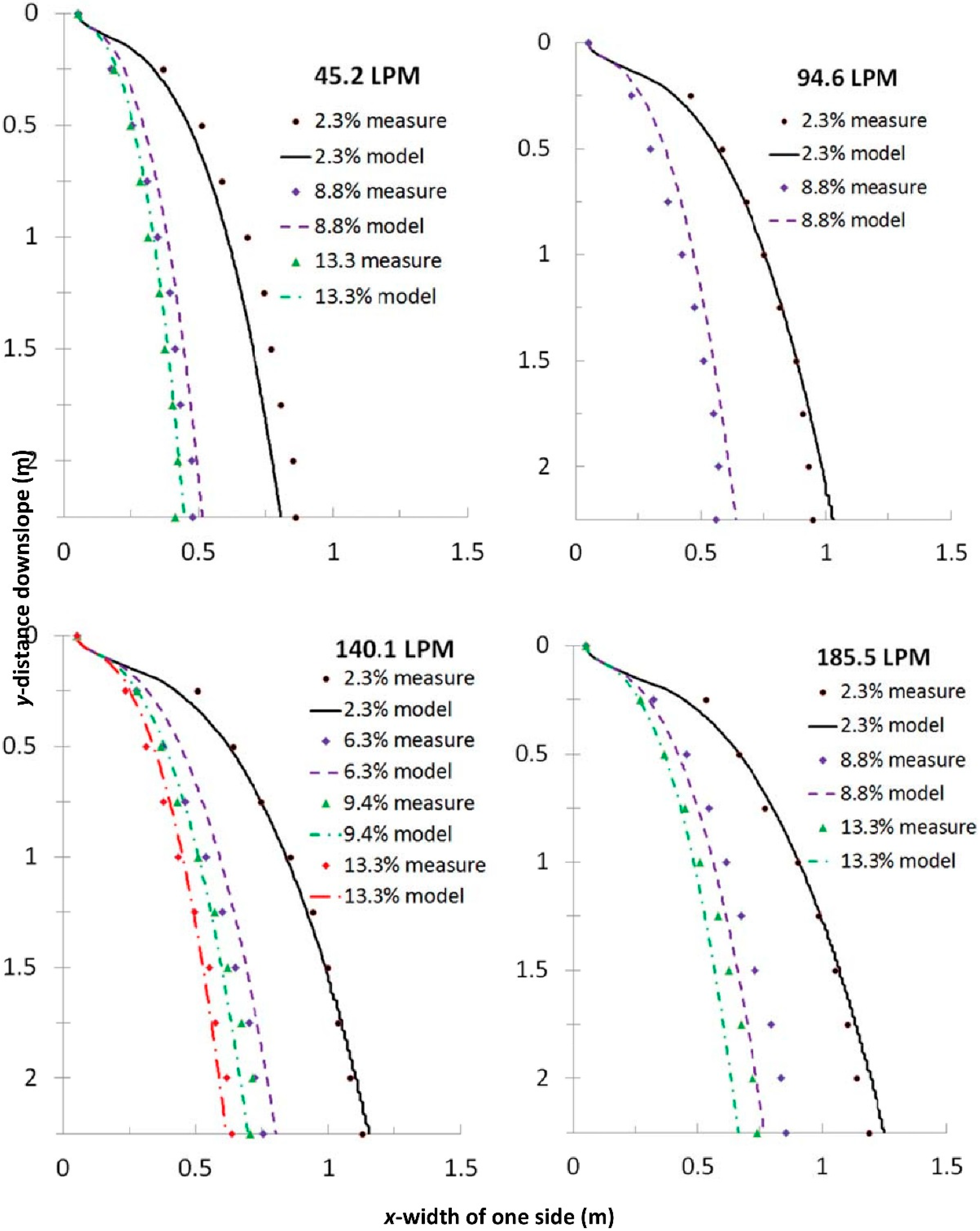
The roughened paint surface was tested first. Figure 2 shows an example of the markers laid out on the grid following a test. Following the tests with various combinations of flowrates and slopes on the painted surface, the system was modeled per the description within the Model section above. The painted surface test n was allowed to vary based on Equation (14) from a base case of n = 0.013 at S = 2.3% (Table 1). This base n value is typical for concrete (Chow, 1959), which was our target roughness created by the addition of sand to the paint. To show the impact of ze on the modeled results, Figure 3 shows predicted solutions of x versus y with Q = 20 LPM, S = 2.3%, x0 = 10.2 cm, n = 0.013, and varying ze. The two largest ze values shown both reach their respective asymptotic widths quickly, whereas the other three smaller ze do not approach their asymptotic width within the 20 m slope modeled.
The test runs for the painted surface were modeled with varying values of ze. The best fit by observation was found for a values of ze = 1.25 mm, which was then used for all subsequent analyses, including both artificial turf surfaces. Figure 4 shows the roughened paint comparison of the measured x versus the modeled x for the various flowrates and slopes with the modified n shown in Table 1, and ze = 1.25 mm. As mentioned above, because symmetry is assumed by the model, all measured x values in this figure, subsequent figures, and resultant statistics are based on the average x from the left and right hand sides of the water plume for each location of y. The modeled lines are concave near the top where the water shoots rapidly out of the trough. The lines quickly change to a convex shape within a distance downslope of approximately 0.2 m, coinciding with the model transitioning from Equation (7) to Equation (10).
Modeling the turf did not require altering n based on slope with Equation (14). This is not surprising, since the height of the water only rarely (at high flowrates and only near the top of the slope) exceeded the height of the resisting artificial blades of grass. A constant n = 0.4 was used to model all slopes of the fine turf (Figure 5) and the coarse turf (Figure 6), which is a value similar to that suggested by the United States Department of Agriculture—National Resource Conservation Service (USDA-NRCS, 1986) for Bermuda grass. The upward concavity of the modeled lines near the top of the slope in Figure 5 and Figure 6 is still present, but is very small as the much larger n caused more rapid spreading, which continued to the bottom of the slope. The ze was again set to 1.25 mm for both the fine and coarse turf.
A summary of the fits for all tests from the three surfaces is shown in Table 2. The primary result of interest is the flow wetted area, since that is what will impact infiltration and is after all the principle purpose of this study. The modeled overall wetted areas from all tests varied absolutely from the measured by a maximum of 12.2% and an average of 5.7%, with no strong trends in the errors. Average absolute errors of 5.2%, 6.0%, and 5.9% were recorded for the roughened painted surface, the fine-bladed artificial turf, and the coarse-bladed artificial turf, respectively.
Initial modeling attempts did not make the simplifying assumption that the energy grade line was equal to the bed slope. Not making this assumption required running the entire model multiple times to establish the energy grade as a function of distance downslope, as this information is not known a priori. Typically, after three to four iterations of solving the model it would stabilize, but not always. Further, the results were always found to be very similar to the first iteration, which did assume that the energy grade line was equal to the bed slope. The decision was therefore made to codify this assumption for all the results presented in this research.
The errors between the measured and modeled areas for each surface and for all three surfaces cumulatively were found to be normally distributed by analysis of their respective normal probability plots, so the standard deviation value in the table can be taken to indicate the likelihood that the area error would be within a certain range. For example, 95% of all modeled errors will be within two standard deviations (so 13.2%) of the measured value.
The wetted area is not the sole result of interest, however, as the modeled area could be accurate without properly describing the plume shape. To ensure this was not occurring, Table 2 also contains for each test the Normalized Mean Absolute Error (NMAEx) for each test run as
where the mod and meas subscripts represent the modeled and measured data, and the denominator describes the average value of x from all y for a given test run. These results show shape differences of the same scale as the areal differences, indicating that the shape is fit about as well as the area. The overall average of all NMAEx was 6.8%. The Root Mean Square Error of x (RMSEx) is also provided in Table 1 for each test. The average RMSEx of all tests was 5.8 cm.
Finally, two different Coefficient of Determinations (R2) were calculated from each test to compare a) the measured left wetted width to the measured right wetted width from all from all y’s, and b) the average measured x (from both the left and right side) from all y’s to that of the model. The R2 values (not shown in Table 1) comparing the measured left and right side wetted width ranged from 0.89 to 1.00, with a mean of 0.99. The R2 values comparing the measured to the modeled data ranged from 0.95 to 1.0 with a mean of 0.98. These two sets of calculations indicate that the left and right hand side of the experiments had very similar wetted shapes, and that these measured wetted shapes were also very similar to those provided by the model.
4. Discussion
As described above, both qualitative and quantitative measures indicate that the model fits the data well for uncalibrated situations. Still, there are questions about how it would be used for actually modeling a storm event being routed from a roof or parking lot over a grassy slope. For example, though above we sometimes describe the model in terms of a “plume”, our use of Manning’s equation limits us to modeling the steady-state condition of area wetted by a constant flow. Of course the model could be applied for serial steady-state conditions at say 15-min intervals, as is common for other stormwater routing routines, but such an approach would add substantial complexity beyond simply calculating the wetted area as a function of time. Assuming infiltration was also being modeled concurrently, the history of infiltration would vary realistically but with great complexity in space and time, as the wetting area initially grows and then recedes along with a runoff event. Alternatively, future research might show that assuming a typical hyetograph shape (e.g., Type II) enables one to select a flow weighted average runoff rate for the entirety of the runoff period to adequately model infiltration with less numerical calculation and complexity. In any case, the approach as presented yields a result of significant use in describing these measures using existing models, and the complexity described above awaits further examination.
Along the same lines, this study did not allow the flow rate to vary down the slope, so that there is no rainfall addition from above nor infiltration removal from below. At the beginning of the event the infiltration rate will likely exceed the rainfall rate. This can happen if a relatively large rooftop area concentrates flow to a smaller infiltration area with most or all of the water infiltrating. Later during the same precipitation event, the potential infiltration rate will decrease due to the soil becoming saturated as the precipitation intensity increases. The generally occurring coincidence of previously wetted soils and high precipitation rates suggests that the percentage error in estimating Q due to infiltration will be smallest when precipitation rate is large and during later times after soils have become wetted. In spite of these caveats, the results of the study are encouraging, particularly the relatively small area errors using uncalibrated textbook n values. The model described in this manuscript is available within the Stormwater Treatment Assessment Resource (STAR), which is an updated version of the Tennessee Runoff Reduction Assessment Tool (TNRRAT, 2015), and it is also available directly from the authors as a macro-enabled Excel 2010 file.
5. Conclusions
A new model is presented that predicts spreading of water released from a downspout or curb cut onto a planar sloped surface with a specific resistance and without infiltration described by a Manning’s n. A comparison of measured versus modeled spreading of water downslope across an approximated concrete slope and two artificial turfs showed good fit. The absolute mean area error from all tests across three surfaces was 5.7%, and based on the standard deviation of the errors 95% of errors associated with predicted wetted areas should be less than 13%. The n values used to predict the spreading were consistent with previously published values, so the model can be applied without prior calibration of n for each surface.
Since the model uses only readily-available information (flow rate, discharge width, slope steepness, and surface material), this approach should provide designers of green infrastructure disconnect measures with realistic estimates of the infiltration area to associate with such practices.
Author Contributions
J.P. and W.C.C. designed and constructed the physical apparatus and conducted the flow testing. J.P. also wrote the Methods section of the manuscript. D.C.Y. initially inspired the project, helped develop the testing protocols, proofed the various numerical models tested, and provided significant editing of the manuscript. J.S.T. oversaw the project, developed the numerical model, and was the lead author of the manuscript.
Funding
The authors would like to thank the funding provided by The University of Tennessee Institute of Agriculture.
Conflicts of Interest
The authors declare no conflicts of interest.
References
- EPA. Green Infrastructure Permitting and Enforcement Series: Factsheet 4; EPA 832F12015; EPA: Washington, DC, USA, 2009.
- EPA. Summary of State Post Construction Stormwater Standards; Office of Water, EPA: Washington, DC, USA, 2016.
- TSM. Tennessee Stormwater Management. 2015. Available online: http://tnpermanentstormwater.org/manual.asp (accessed on 9 October 2017).
- Coussat, P.; Proust, S. Slow, unconfined spreading of a mudflow. J. Geophys. Res. 1996, 101, 217–229. [Google Scholar] [CrossRef]
- Schmitz, G.H.; Seus, G.J. Analytical model of level basin irrigation. J. Irrig. Drain. Eng. 1989, 115, 78–95. [Google Scholar] [CrossRef]
- EPA. National Stormwater Calculator User’s Guide. 2010. Available online: http://www.epa.gov/nrmrl/wswrd/wq/models/swc/ (accessed on 14 September 2017).
- TNRRAT. Tennessee Runoff Reduction. 2015. Available online: www.tnpermanentstormwater.org/TNRRAT.asp (accessed on 9 October 2017).
- Singh, V.; Bhallamudi, S.M. Hydrodynamic modeling of basin irrigation. J. Irrig. Drain. Eng. 1997, 123, 407–414. [Google Scholar] [CrossRef]
- Guardo, M.; Oad, R.; Podmore, T.H. Comparison of zero-inertia and volume balance advance-infiltration models. J. Hydraul. Eng. 2000, 126, 457–465. [Google Scholar] [CrossRef]
- Strelkoff, T.S.; Tamimi, A.H.; Clemmens, A.J. Two-dimensional basin flow with irregular bottom configuration. J. Irrig. Drain. Eng. 2003, 129, 391–401. [Google Scholar] [CrossRef]
- Ebrahimian, H.; Liaghat, A.; Parsinejad, M.; Abbasi, F.; Navabian, M. Comparison of one- and two-dimensional models to simulate alternate and conventional furrow fertigation. J. Irrig. Drain. Eng. 2012, 138, 929–938. [Google Scholar] [CrossRef]
- Manning, R. On the flow of water in open channels and pipes. Trans. Inst. Civ. Eng. Irel. Dublin 1891, 20, 161–207. [Google Scholar]
- Chow, V.T. Open-Channel Hydraulics; McGraw-Hill: New York, NY, USA, 1959. [Google Scholar]
- USDA-NRCS. Urban hydrology for small watersheds. In Technical Release, 2nd ed.; Conservation Engineering Division, NRCS: Washington, DC, USA, 1986. [Google Scholar]
- Reed, J.; Kibler, D. Hydraulic resistance of pavement surfaces. J. Transp. Eng. 1983, 109, 286–296. [Google Scholar] [CrossRef]
- Simmons, C.S.; Keller, J.M.; Hylden, J.L. Spills on Flat Inclined Pavement; PNNL-14577; Pacific Northwest Laboratory: Washington, DC, USA, 2004. [Google Scholar]
- Yoder, D.C.; Wilkerson, J.B.; Buchanan, J.R.; Hurley, K.J.; Yoder, R.E. Development and evaluation of a device to control time varying flows. Trans. ASAE 1998, 41, 325–332. [Google Scholar] [CrossRef]
Figure 1.
Cross sectional profile for modeled flow down the slope.

Figure 2.
The physical test apparatus for measuring the area of water spread from a 10.2 cm (4 in.) discharge width onto a platform, in this case with a roughened painted surface. Grid lines are at 25-cm spacing in both directions. The black dots are pennies placed by hand to mark the greatest extent of wetting observed during the run.

Figure 3.
Modeled width of flow spread as a function of ze with Q = 20 LPM, S = 2.3%, x0 = 10.2 cm, and n = 0.013.
Figure 3.
Modeled width of flow spread as a function of ze with Q = 20 LPM, S = 2.3%, x0 = 10.2 cm, and n = 0.013.

Figure 4.
Measured and modeled results of one side of the water spreading onto a roughened painted surface for varying Q and Sy with x0 = 10.2 cm and n varying with slope as per Equation (14). The measured x values are the average of the right and left sides at that value of y.
Figure 4.
Measured and modeled results of one side of the water spreading onto a roughened painted surface for varying Q and Sy with x0 = 10.2 cm and n varying with slope as per Equation (14). The measured x values are the average of the right and left sides at that value of y.

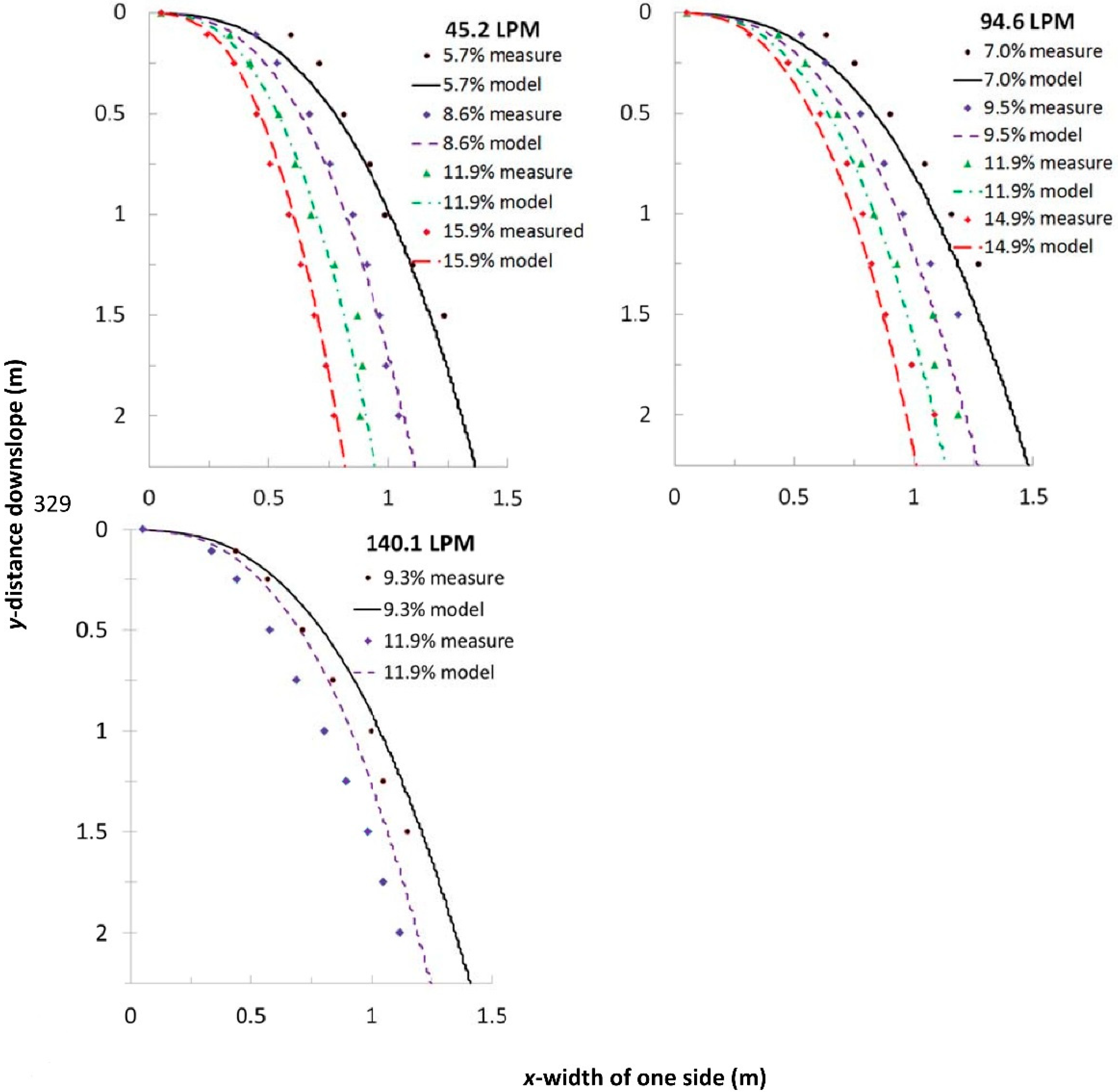
Figure 5.
Measured and modeled results of one side of the water spreading onto a fine bladed artificial turf for varying Q and Sy with x0 = 10.2 cm. The measured x values are the average of the right and left sides at that value of y.
Figure 5.
Measured and modeled results of one side of the water spreading onto a fine bladed artificial turf for varying Q and Sy with x0 = 10.2 cm. The measured x values are the average of the right and left sides at that value of y.

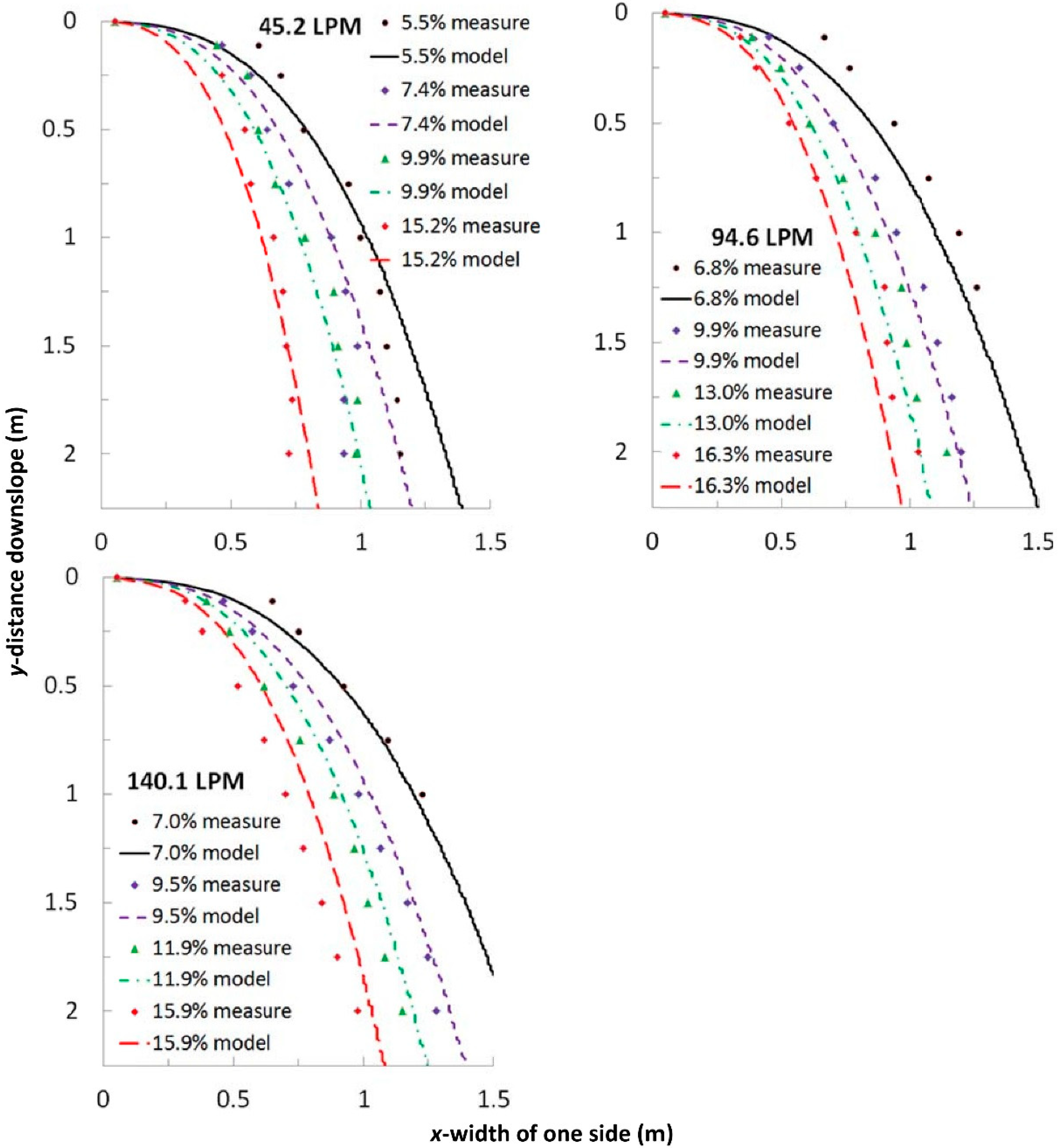
Figure 6.
Measured and modeled results of one-side of the water spreading onto a coarse bladed artificial turf for varying Q and Sy with x0 = 10.2 cm. The measured x values are the average of the right and left sides at that value of y.
Figure 6.
Measured and modeled results of one-side of the water spreading onto a coarse bladed artificial turf for varying Q and Sy with x0 = 10.2 cm. The measured x values are the average of the right and left sides at that value of y.


Table 1.
Calculated n from Sy for the roughened paint surface, based on Equation (14).
| Sy | 2.3% | 6.3% | 8.8% | 9.4% | 13.3% | 15.9% |
| n | 0.013 | 0.021 | 0.025 | 0.026 | 0.031 | 0.034 |
Table 2.
Summary statistics of results from measured and modeled testing.
| Surface | Flowrate (LPM) | Slope % | Area Measure (m2) | Area Model (m2) | Area Error | NMAEx * | RMSEx ** (cm) |
|---|---|---|---|---|---|---|---|
| Roughened Paint | 45.2 | 2.3 | 2.89 | 2.61 | −9.5% | 8.9% | 6.3 |
| 8.8 | 1.54 | 1.67 | 8.4% | 9.1% | 3.4 | ||
| 13.3 | 1.41 | 1.45 | 2.6% | 3.8% | 1.5 | ||
| 94.6 | 2.3 | 3.25 | 3.26 | 0.4% | 4.0% | 4.2 | |
| 8.8 | 1.87 | 2.05 | 9.7% | 10.7% | 4.9 | ||
| 140.1 | 2.3 | 3.69 | 3.63 | −1.6% | 2.5% | 3.1 | |
| 6.3 | 2.37 | 2.56 | 8.0% | 8.4% | 4.9 | ||
| 9.4 | 2.27 | 2.22 | −2.5% | 3.6% | 2.4 | ||
| 13.3 | 1.97 | 1.96 | −0.5% | 4.0% | 2.0 | ||
| 185.5 | 2.3 | 3.88 | 3.91 | 0.8% | 3.6% | 4.4 | |
| 8.8 | 2.71 | 2.44 | −10.2% | 9.8% | 6.9 | ||
| 13.3 | 2.30 | 2.10 | −8.3% | 8.0% | 5.4 | ||
| abs. mean 5.2% | mean 6.4% | mean 4.1 | |||||
| fine turf | 45.2 | 5.5 | 2.64 | 2.51 | −5.0% | 6.6% | 8.2 |
| 8.6 | 3.16 | 3.06 | −3.1% | 4.3% | 4.3 | ||
| 11.9 | 2.66 | 2.60 | −1.9% | 3.7% | 2.9 | ||
| 15.9 | 2.20 | 2.25 | 2.4% | 2.7% | 7.5 | ||
| 94.6 | 7 | 2.32 | 2.10 | −9.5% | 10.2% | 10.5 | |
| 9.5 | 2.52 | 2.33 | −7.5% | 8.4% | 8.1 | ||
| 11.9 | 3.32 | 3.11 | −6.2% | 6.8% | 6.6 | ||
| 14.9 | 2.94 | 2.78 | −5.5% | 5.7% | 5.4 | ||
| 140.1 | 9.3 | 2.43 | 2.59 | 6.6% | 6.5% | 6.1 | |
| 11.9 | 3.04 | 3.42 | 12.2% | 12.1% | 0.9 | ||
| abs. mean 6.0% | mean 6.7% | mean 6.1 | |||||
| course turf | 45.2 | 5.5 | 3.73 | 3.82 | 2.4% | 8.9% | 10.3 |
| 7.4 | 3.13 | 3.30 | 5.2% | 9.7% | 10.0 | ||
| 9.9 | 3.01 | 2.85 | −5.1% | 6.2% | 6.2 | ||
| 15.2 | 2.40 | 2.28 | −5.0% | 7.5% | 6.0 | ||
| 94.6 | 6.8 | 2.39 | 2.13 | −10.6% | 11.1% | 11.8 | |
| 9.9 | 3.56 | 3.41 | −4.1% | 4.1% | 4.2 | ||
| 13 | 3.18 | 2.98 | −6.3% | 6.6% | 6.2 | ||
| 16.3 | 2.85 | 2.65 | −6.9% | 8.0% | 7.1 | ||
| 140.1 | 7 | 1.77 | 1.68 | −4.9% | 5.8% | 7.6 | |
| 9.5 | 3.70 | 3.82 | 3.5% | 4.2% | 4.1 | ||
| 11.9 | 3.24 | 3.42 | 5.5% | 5.7% | 5.1 | ||
| 15.9 | 2.65 | 2.95 | 11.5% | 11.1% | 7.9 | ||
| abs. mean 5.9% | mean 7.4% | mean 7.2 | |||||
| all data | abs. mean 5.7% | mean 6.8% | mean 5.8 | ||||
| st. dev. 6.6% | |||||||
* NMAEx = Normalized Mean Absolute Error of x. ** RMSEx = Root Mean Square Error of x.
© 2018 by the authors. Licensee MDPI, Basel, Switzerland. This article is an open access article distributed under the terms and conditions of the Creative Commons Attribution (CC BY) license (http://creativecommons.org/licenses/by/4.0/).
Share and Cite
MDPI and ACS Style
Tyner, J.S.; Yoder, D.C.; Parker, J.; Credille, W.C. Estimating the Infiltration Area for Concentrated Stormwater Spreading over Grassed and Other Slopes. Water 2018, 10, 1200. https://doi.org/10.3390/w10091200
AMA Style
Tyner JS, Yoder DC, Parker J, Credille WC. Estimating the Infiltration Area for Concentrated Stormwater Spreading over Grassed and Other Slopes. Water. 2018; 10(9):1200. https://doi.org/10.3390/w10091200
Chicago/Turabian StyleTyner, John S., Daniel C. Yoder, Jacob Parker, and William C. Credille. 2018. "Estimating the Infiltration Area for Concentrated Stormwater Spreading over Grassed and Other Slopes" Water 10, no. 9: 1200. https://doi.org/10.3390/w10091200
Note that from the first issue of 2016, this journal uses article numbers instead of page numbers. See further details here.