New Hybrids of ANFIS with Several Optimization Algorithms for Flood Susceptibility Modeling

 ,
,  ,
,  , ,
, ,  , ,
, ,
Abstract
:
1. Introduction
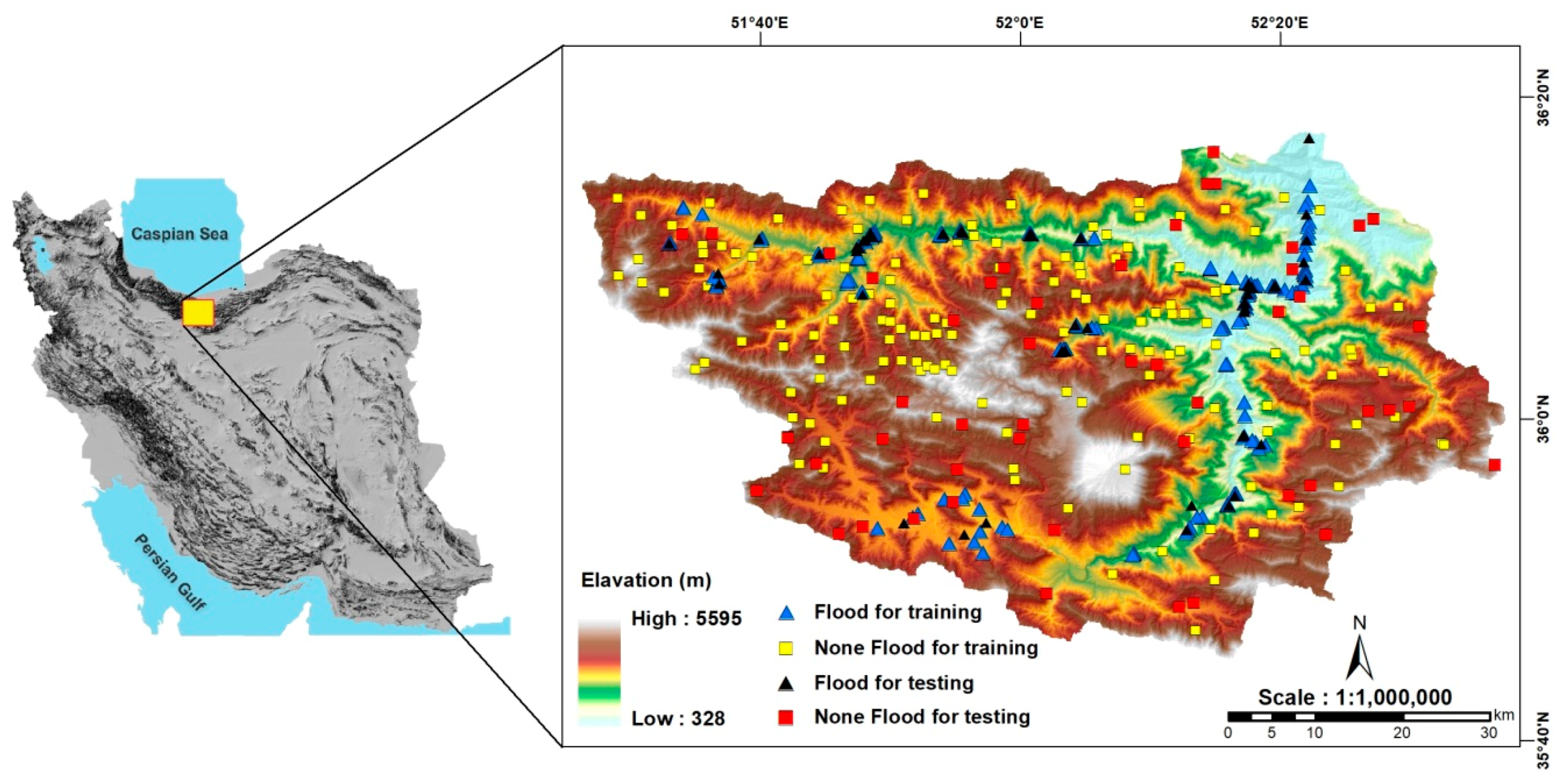
2. Study Area
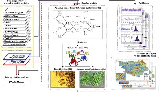
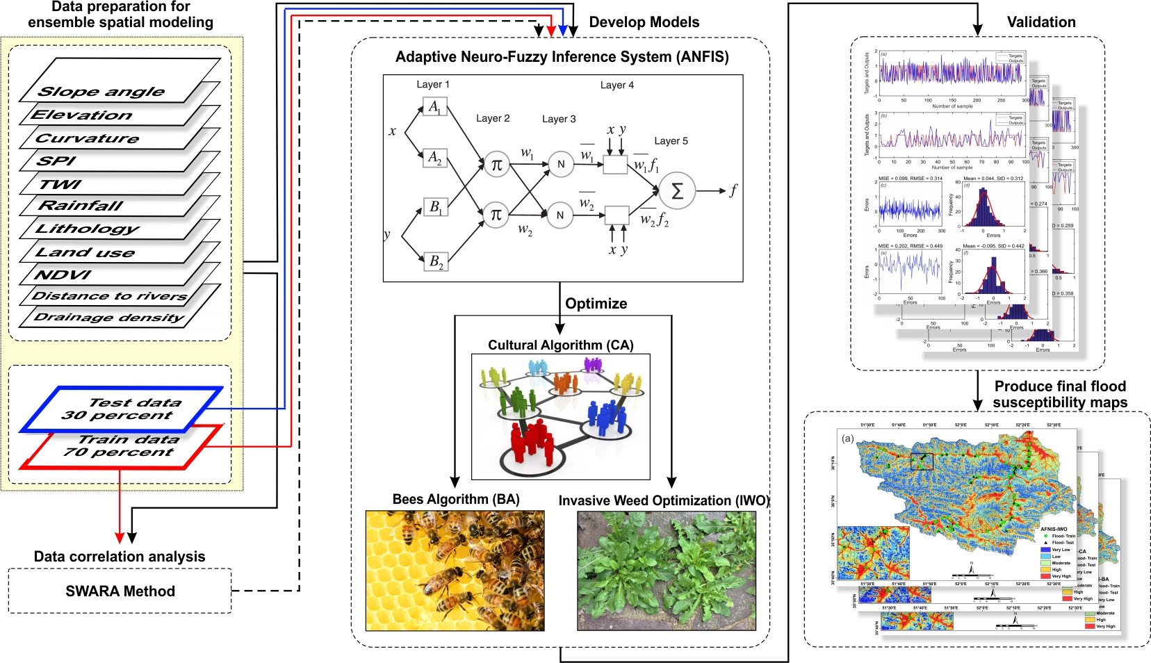
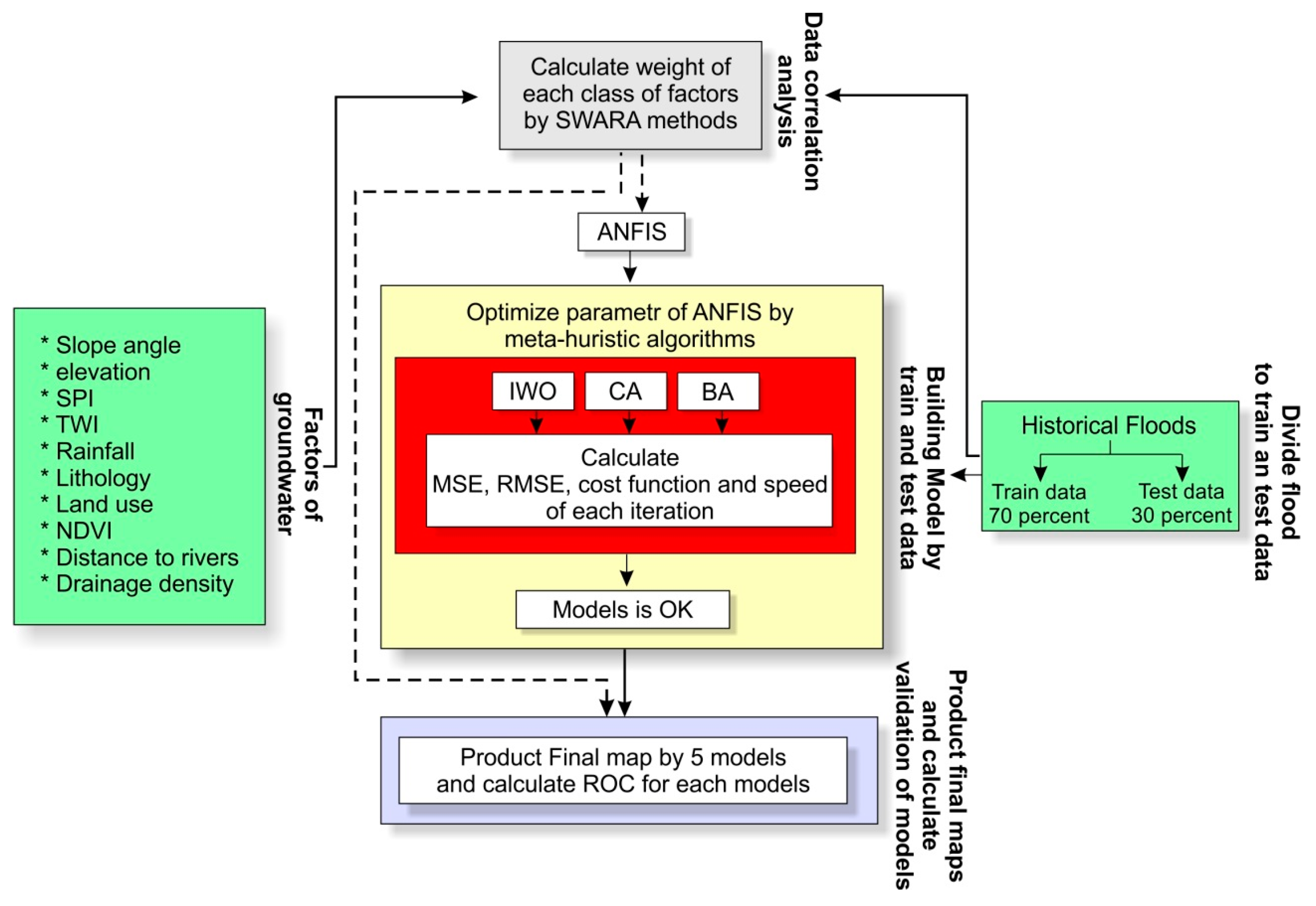
3. Data Preparation and Analysis
3.1. Flash Flood Inventory
3.2. Dataset Collection for Spatial Modeling
3.3. Preparation of Training and Testing Dataset
3.4. Analysis of Spatial Correlation
3.5. Flood Spatial Prediction Modeling
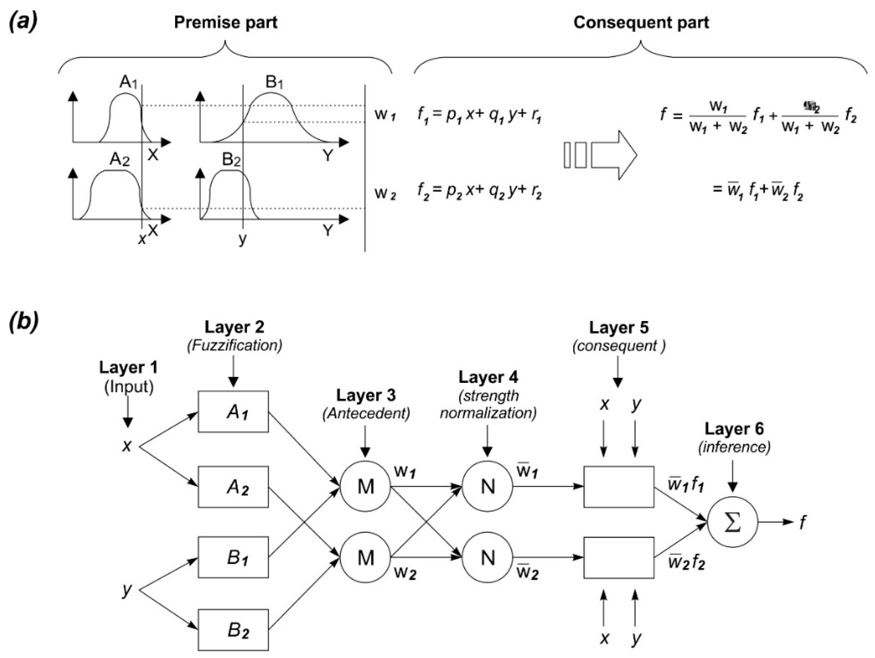
3.5.1. Adaptive Neuro-Fuzzy Inference System
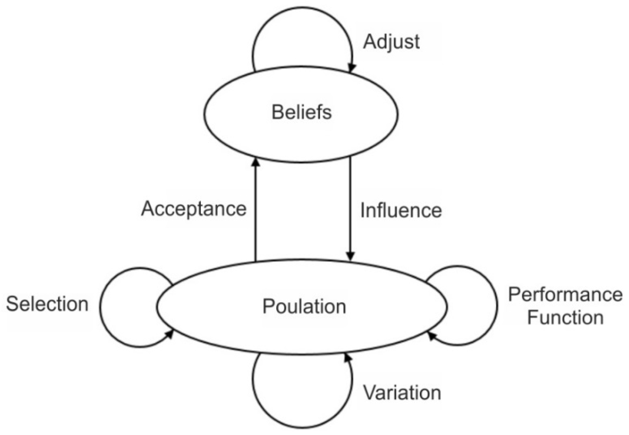
3.5.2. Cultural Algorithm
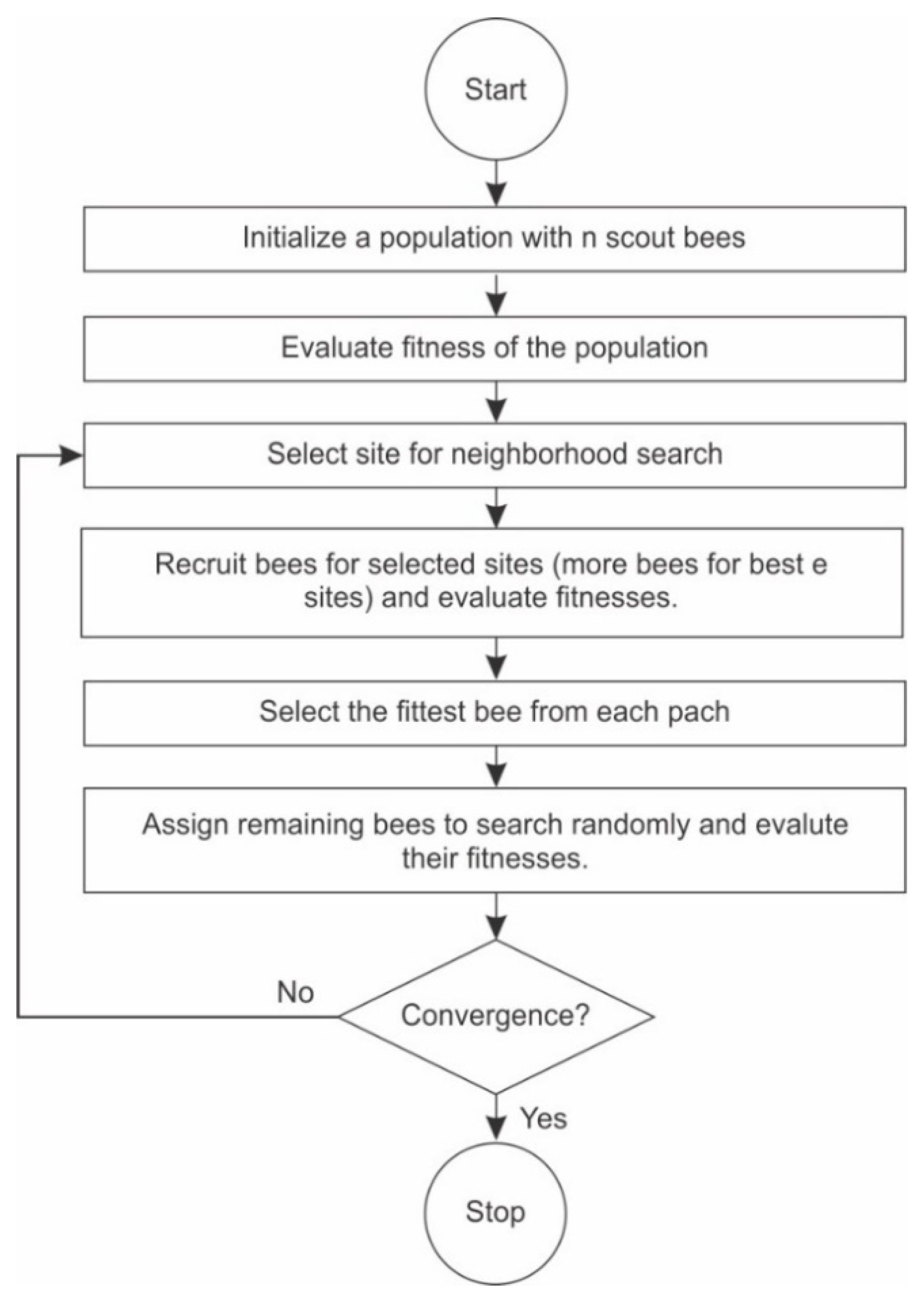
3.5.3. Bees Algorithm
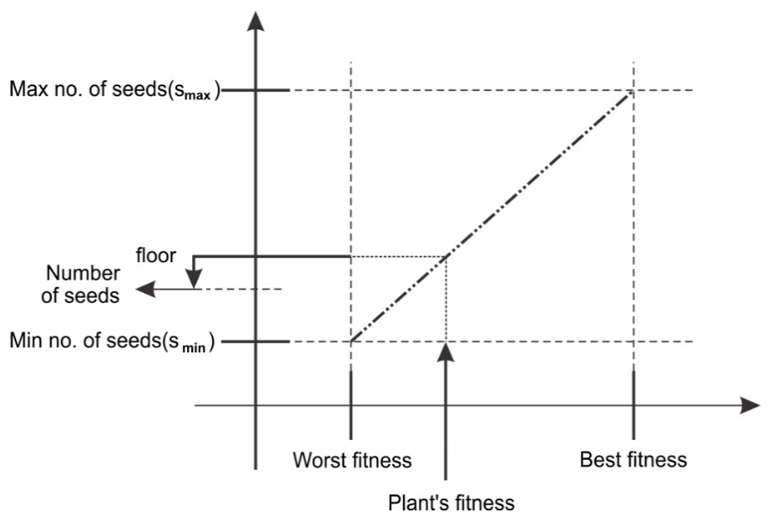
3.5.4. Invasive Weed Optimization Algorithm
3.5.5. Performance Assessment
3.6. Model Validation and Comparisons
3.7. Inferential Statistics
3.7.1. Freidman Test
3.7.2. Wilcoxon Test
4. Results
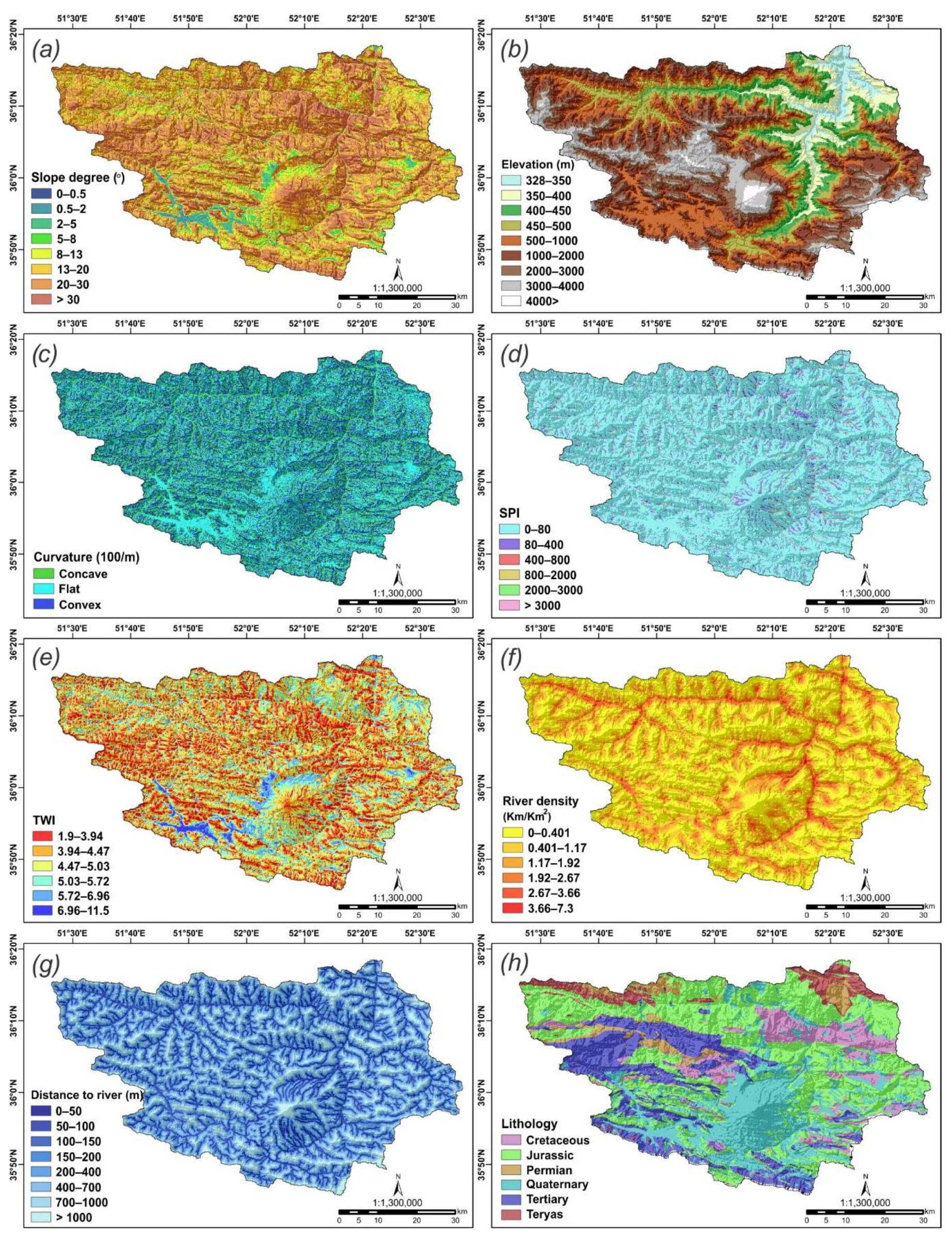
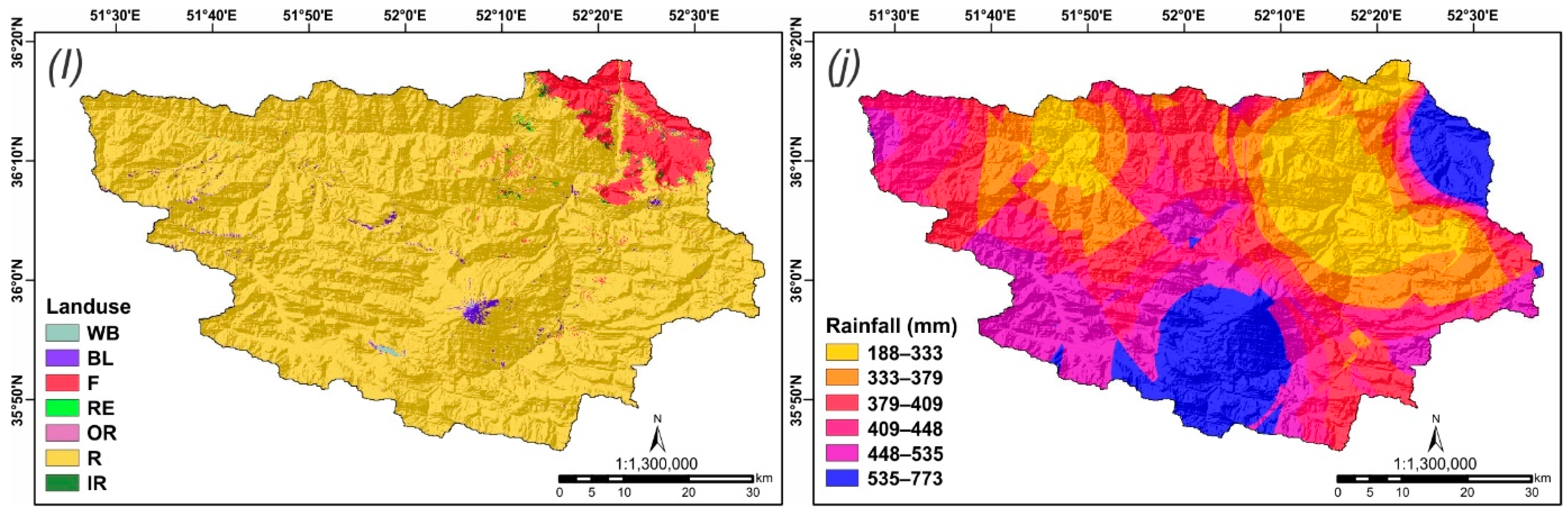
4.1. Spatial Relationship between Flood Occurrence and Conditioning Factors
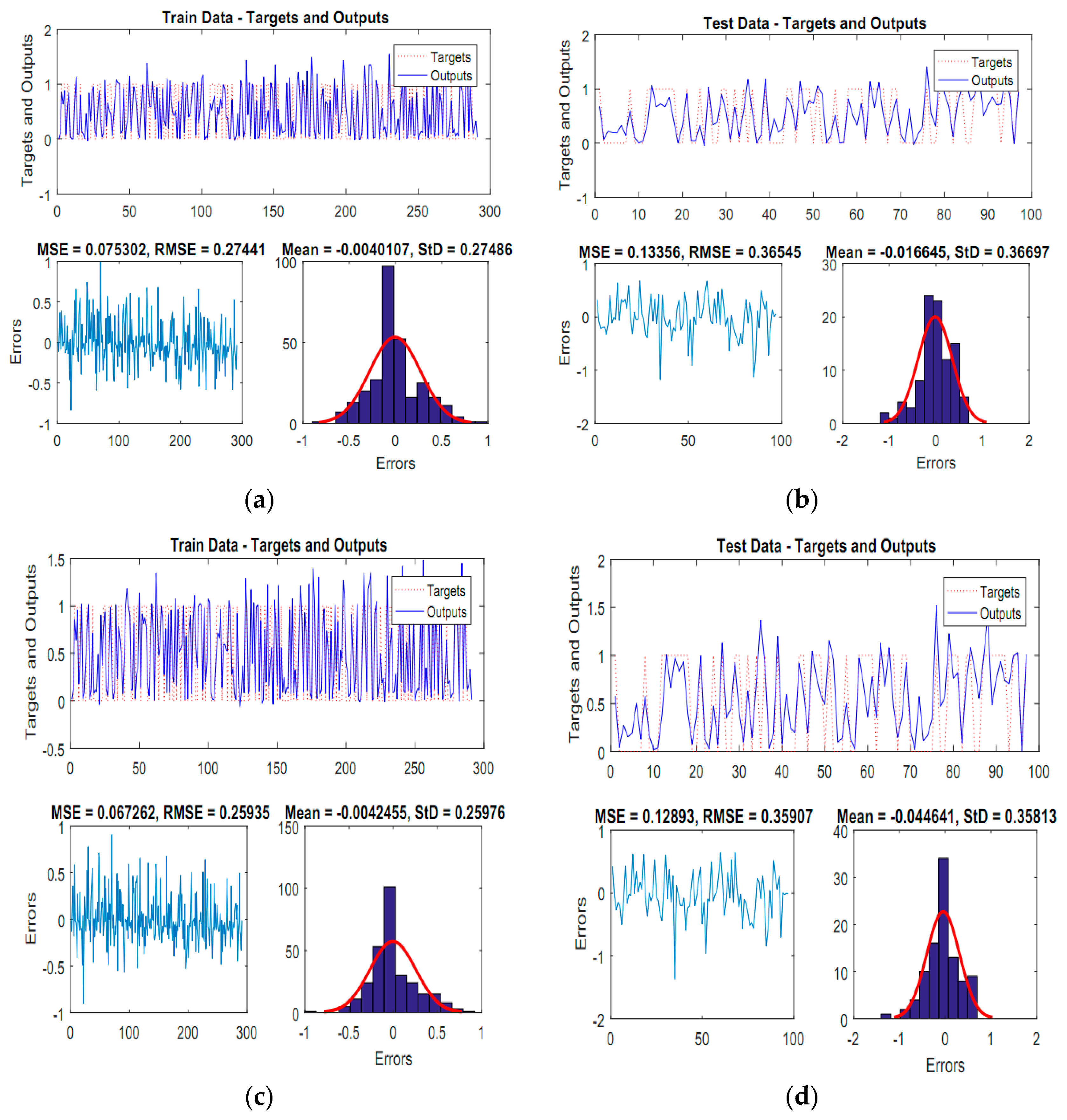
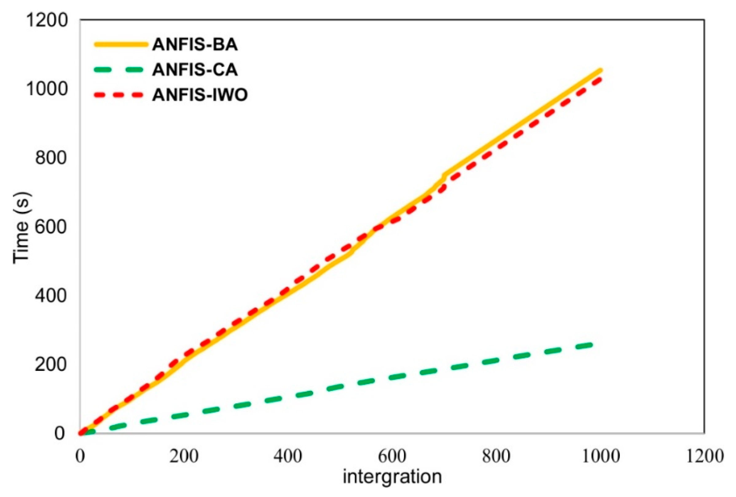
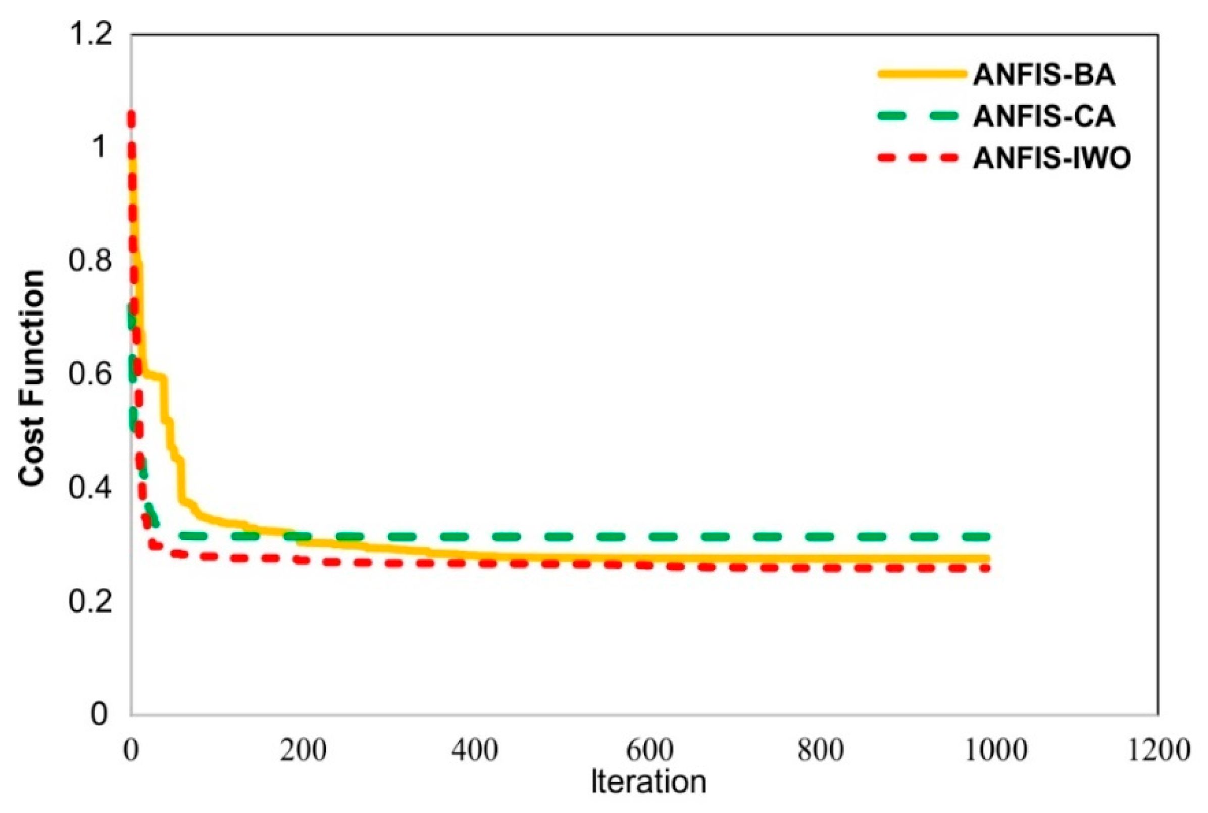
4.2. Model Comparison between the Proposed New ANFIS Ensemble Models
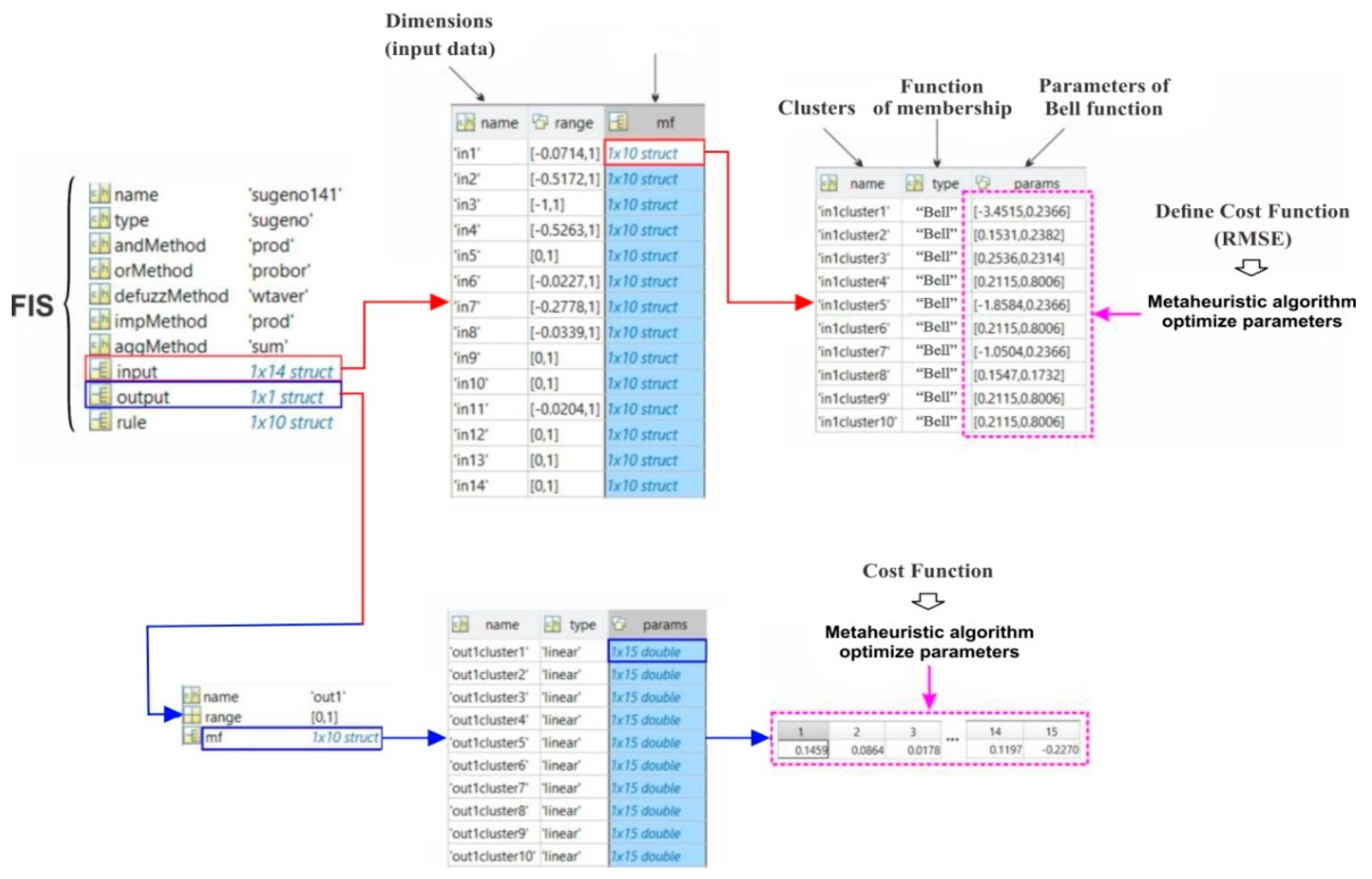
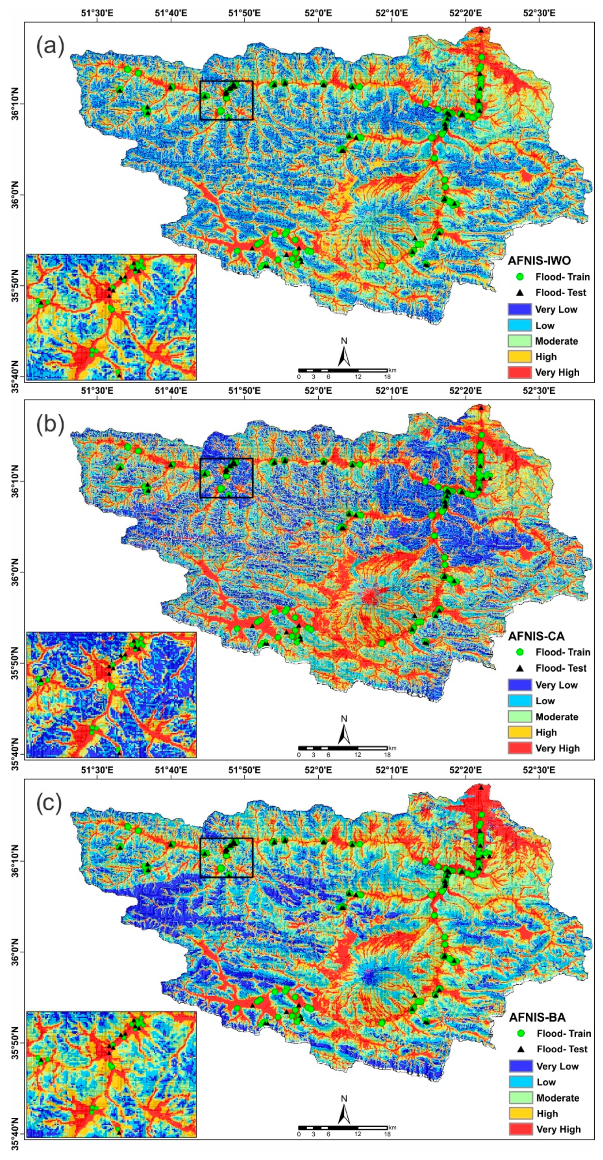
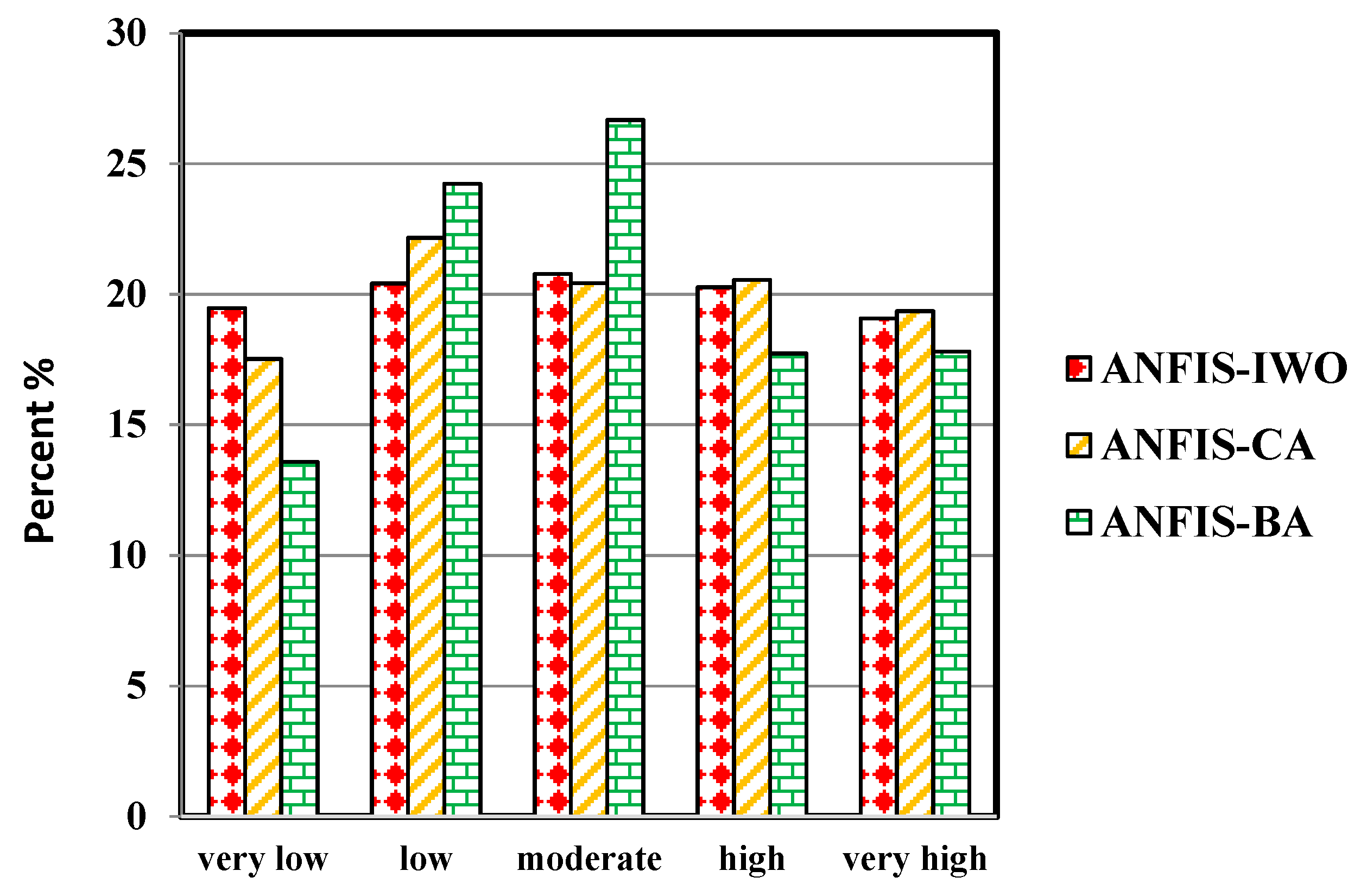
4.3. Model Configuration and Generating of FSMs Using ANFIS Ensemble Models
4.4. Validation of Flood Susceptibility Maps
5. Discussion
6. Conclusions
Author Contributions
Funding
Acknowledgments
Conflicts of Interest
References
- Elkhrachy, I. Flash flood hazard mapping using satellite images and GIS tools: A case study of Najran City, Kingdom of Saudi Arabia (KSA). Egypt. J. Remote Sens. Space. Sci. 2015, 18, 261–278. [Google Scholar] [CrossRef]
- Tehrany, M.S.; Pradhan, B.; Jebur, M.N. Flood susceptibility analysis and its verification using a novel ensemble support vector machine and frequency ratio method. Stoch. Environ. Res. Risk Assess. 2015, 29, 1149–1165. [Google Scholar] [CrossRef]
- Youssef, A.M.; Pradhan, B.; Hassan, A.M. Flash flood risk estimation along the St. Katherine road, southern Sinai, Egypt using GIS based morphometry and satellite imagery. Environ. Earth Sci. 2011, 62, 611–623. [Google Scholar] [CrossRef]
- Lee, E.H.; Kim, J.H.; Choo, Y.M.; Jo, D.J. Application of flood nomograph for flood forecasting in urban areas. Water 2018, 10, 53. [Google Scholar] [CrossRef]
- Sarhadi, A.; Soltani, S.; Modarres, R. Probabilistic flood inundation mapping of ungauged rivers: Linking GIS techniques and frequency analysis. J. Hydrol. 2012, 458, 68–86. [Google Scholar] [CrossRef]
- Luu, C.; von Meding, J. A flood risk assessment of quang nam, vietnam using spatial multicriteria decision analysis. Water 2018, 10, 461. [Google Scholar] [CrossRef]
- Dutta, D.; Herath, S. Trend of Floods in Asia and Flood Risk Management with Integrated River Basin Approach. In Proceedings of the 2nd APHW Conference, Singapore, 5–8 July 2004; pp. 55–63. [Google Scholar]
- Smith, K. Environmental Hazards: Assessing Risk and Reducing Disaster; Routledge: London, UK, 2013. [Google Scholar]
- Khosravi, K.; Nohani, E.; Maroufinia, E.; Pourghasemi, H.R. A GIS-based flood susceptibility assessment and its mapping in iran: A comparison between frequency ratio and weights-of-evidence bivariate statistical models with multi-criteria decision-making technique. Nat. Hazards 2016, 83, 947–987. [Google Scholar] [CrossRef]
- Khosravi, K.; Pourghasemi, H.R.; Chapi, K.; Bahri, M. Flash flood susceptibility analysis and its mapping using different bivariate models in Iran: A comparison between Shannon’s entropy, statistical index, and weighting factor models. Environ. Monit. Assess. 2016, 188, 656. [Google Scholar] [CrossRef] [PubMed]
- Shafizadeh-Moghadam, H.; Valavi, R.; Shahabi, H.; Chapi, K.; Shirzadi, A. Novel forecasting approaches using combination of machine learning and statistical models for flood susceptibility mapping. J. Environ. Manag. 2018, 217, 1–11. [Google Scholar] [CrossRef] [PubMed]
- Chapi, K. Monitoring and Modeling of Runoff Generating Areas in a Small Agricultural Watershed. Ph.D. Thesis, University of Guelph, Guelph, Canada, 2010. [Google Scholar]
- Chapi, K.; Rudra, R.P.; Ahmed, S.I.; Khan, A.A.; Gharabaghi, B.; Dickinson, W.T.; Goel, P.K. Spatial-temporal dynamics of runoff generation areas in a small agricultural watershed in southern Ontario. J. Water Resour. Prot. 2015, 7, 14–40. [Google Scholar] [CrossRef]
- Fenicia, F.; Kavetski, D.; Savenije, H.H.; Clark, M.P.; Schoups, G.; Pfister, L.; Freer, J. Catchment properties, function, and conceptual model representation: Is there a correspondence? Hydrol. Process. 2014, 28, 2451–2467. [Google Scholar] [CrossRef]
- Kisi, O.; Nia, A.M.; Gosheh, M.G.; Tajabadi, M.R.J.; Ahmadi, A. Intermittent streamflow forecasting by using several data driven techniques. Water Resour. Manag. 2012, 26, 457–474. [Google Scholar] [CrossRef]
- Ganguli, P.; Reddy, M.J. Probabilistic assessment of flood risks using trivariate copulas. Theor. Appl. Climatol. 2013, 111, 341–360. [Google Scholar] [CrossRef]
- Refsgaard, J.C. Parameterisation, calibration and validation of distributed hydrological models. J. Hydrol. 1997, 198, 69–97. [Google Scholar] [CrossRef]
- Cea, L.; Bladé, E. A simple and efficient unstructured finite volume scheme for solving the shallow water equations in overland flow applications. Water Resour. Res. 2015, 51, 5464–5486. [Google Scholar] [CrossRef] [Green Version]
- Costabile, P.; Costanzo, C.; Macchione, F. A storm event watershed model for surface runoff based on 2D fully dynamic wave equations. Hydrol. Process. 2013, 27, 554–569. [Google Scholar] [CrossRef]
- Xia, X.; Liang, Q.; Ming, X.; Hou, J. An efficient and stable hydrodynamic model with novel source term discretization schemes for overland flow and flood simulations. Water Resour. Res. 2017, 53, 3730–3759. [Google Scholar] [CrossRef] [Green Version]
- Bellos, V.; Tsakiris, G. A hybrid method for flood simulation in small catchments combining hydrodynamic and hydrological techniques. J. Hydrol. 2016, 540, 331–339. [Google Scholar] [CrossRef]
- Liang, D.; Özgen, I.; Hinkelmann, R.; Xiao, Y.; Chen, J.M. Shallow water simulation of overland flows in idealised catchments. Environ. Earth Sci. 2015, 74, 7307–7318. [Google Scholar] [CrossRef] [Green Version]
- Singh, J.; Altinakar, M.S.; Ding, Y. Numerical modeling of rainfall-generated overland flow using nonlinear shallow-water equations. J. Hydrol. Eng. 2014, 20. [Google Scholar] [CrossRef]
- Rahmati, O.; Naghibi, S.A.; Shahabi, H.; Bui, D.T.; Pradhan, B.; Azareh, A.; Rafiei-Sardooi, E.; Samani, A.N.; Melesse, A.M. Groundwater spring potential modelling: comprising the capability and robustness of three different modeling approaches. J. Hydrol. 2018, 565, 248–261. [Google Scholar] [CrossRef]
- Bui, D.T.; Pradhan, B.; Nampak, H.; Bui, Q.-T.; Tran, Q.-A.; Nguyen, Q.-P. Hybrid artificial intelligence approach based on neural fuzzy inference model and metaheuristic optimization for flood susceptibilitgy modeling in a high-frequency tropical cyclone area using GIS. J. Hydrol. 2016, 540, 317–330. [Google Scholar]
- Tyrna, B.; Assmann, A.; Fritsch, K.; Johann, G. Large-scale high-resolution pluvial flood hazard mapping using the raster-based hydrodynamic two-dimensional model flood FloodAreaHPC. J. Flood Risk Manag. 2018, 11, S1024–S1037. [Google Scholar] [CrossRef]
- Al-Abadi, A.M.; Shahid, S.; Al-Ali, A.K. A GIS-based integration of catastrophe theory and analytical hierarchy process for mapping flood susceptibility: A case study of teeb area, southern Iraq. Environ. Earth Sci. 2016, 75, 1–19. [Google Scholar] [CrossRef]
- Tehrany, M.S.; Pradhan, B.; Jebur, M.N. Flood susceptibility mapping using a novel ensemble weights-of-evidence and support vector machine models in GIS. J. Hydrol. 2014, 512, 332–343. [Google Scholar] [CrossRef]
- Tehrany, M.S.; Pradhan, B.; Mansor, S.; Ahmad, N. Flood susceptibility assessment using GIS-based support vector machine model with different kernel types. Catena. 2015, 125, 91–101. [Google Scholar] [CrossRef]
- Youssef, A.M.; Pradhan, B.; Sefry, S.A. Flash flood susceptibility assessment in Jeddah city (Kingdom of Saudi Arabia) using bivariate and multivariate statistical models. Environ. Earth Sci. 2016, 75, 12. [Google Scholar] [CrossRef]
- Fotopoulos, F.; Makropoulos, C.; Mimikou, M.A. Validation of satellite rainfall products for operational flood forecasting: The case of the Evros catchment. Theor. Appl. Climatol. 2011, 104, 403–414. [Google Scholar] [CrossRef]
- Tehrany, M.S.; Pradhan, B.; Jebur, M.N. Spatial prediction of flood susceptible areas using rule based decision tree (DT) and a novel ensemble bivariate and multivariate statistical models in GIS. J. Hydrol. 2013, 504, 69–79. [Google Scholar] [CrossRef] [Green Version]
- Pradhan, B. Flood susceptible mapping and risk area delineation using logistic regression, GIS and remote sensing. J. Spatial Hydrol. 2010, 9, 1–18. [Google Scholar]
- Gigović, L.; Pamučar, D.; Bajić, Z.; Drobnjak, S. Application of GIS-interval rough AHP methodology for flood hazard mapping in urban areas. Water 2017, 9, 360. [Google Scholar] [CrossRef]
- Kia, M.B.; Pirasteh, S.; Pradhan, B.; Mahmud, A.R.; Sulaiman, W.N.A.; Moradi, A. An artificial neural network model for flood simulation using GIS: Johor River Basin, Malaysia. Environ. Earth Sci. 2012, 67, 251–264. [Google Scholar] [CrossRef]
- Khosravi, K.; Pham, B.T.; Chapi, K.; Shirzadi, A.; Shahabi, H.; Revhaug, I.; Prakash, I.; Bui, D.T. A comparative assessment of decision trees algorithms for flash flood susceptibility modeling at Haraz watershed, northern Iran. Sci. Total Environ. 2018, 627, 744–755. [Google Scholar] [CrossRef] [PubMed]
- Hong, H.; Panahi, M.; Shirzadi, A.; Ma, T.; Liu, J.; Zhu, A.-X.; Chen, W.; Kougias, I.; Kazakis, N. Flood susceptibility assessment in Hengfeng area coupling adaptive neuro-fuzzy inference system with genetic algorithm and differential evolution. Sci. Total Environ. 2017, 621, 1124–1141. [Google Scholar] [CrossRef] [PubMed]
- Chapi, K.; Singh, V.P.; Shirzadi, A.; Shahabi, H.; Bui, D.T.; Pham, B.T.; Khosravi, K. A novel hybrid artificial intelligence approach for flood susceptibility assessment. Environ. Model. Softw. 2017, 95, 229–245. [Google Scholar] [CrossRef]
- Termeh, S.V.R.; Kornejady, A.; Pourghasemi, H.R.; Keesstra, S. Flood susceptibility mapping using novel ensembles of adaptive neuro fuzzy inference system and metaheuristic algorithms. Sci. Total Environ. 2018, 615, 438–451. [Google Scholar] [CrossRef] [PubMed]
- Maier, H.R.; Jain, A.; Dandy, G.C.; Sudheer, K.P. Methods used for the development of neural networks for the prediction of water resource variables in river systems: Current status and future directions. Environ. Model. Softw. 2010, 25, 891–909. [Google Scholar] [CrossRef]
- Dottori, F.; Martina, M.L.V.; Figueiredo, R. A methodology for flood susceptibility and vulnerability analysis in complex flood scenarios. J. Flood Risk Manag. 2018, 11, S632–S645. [Google Scholar] [CrossRef]
- Ghalkhani, H.; Golian, S.; Saghafian, B.; Farokhnia, A.; Shamseldin, A. Application of surrogate artificial intelligent models for real-time flood routing. Water Environ. J. 2013, 27, 535–548. [Google Scholar] [CrossRef]
- Rezaeianzadeh, M.; Tabari, H.; Yazdi, A.A.; Isik, S.; Kalin, L. Flood flow forecasting using ANN, ANFIS and regression models. Neural Comput. Appl. 2014, 25, 25–37. [Google Scholar] [CrossRef]
- Chang, F.-J.; Tsai, M.-J. A nonlinear spatio-temporal lumping of radar rainfall for modeling multi-step-ahead inflow forecasts by data-driven techniques. J. Hydrol. 2016, 535, 256–269. [Google Scholar] [CrossRef]
- Güçlü, Y.S.; Şen, Z. Hydrograph estimation with fuzzy chain model. J. Hydrol. 2016, 538, 587–597. [Google Scholar] [CrossRef]
- Lohani, A.; Kumar, R.; Singh, R. Hydrological time series modeling: A comparison between adaptive neuro-fuzzy, neural network and autoregressive techniques. J. Hydrol. 2012, 442, 23–35. [Google Scholar] [CrossRef]
- Shu, C.; Ouarda, T. Regional flood frequency analysis at ungauged sites using the adaptive neuro-fuzzy inference system. J. Hydrol. 2008, 349, 31–43. [Google Scholar] [CrossRef]
- Mukerji, A.; Chatterjee, C.; Raghuwanshi, N.S. Flood forecasting using ANN, Neuro-Fuzzy, and Neuro-GA models. J. Hydrol. Eng. 2009, 14, 647–652. [Google Scholar] [CrossRef]
- Nayak, P.C.; Sudheer, K.P.; Rangan, D.M.; Ramasastri, K.S. Short-term flood forecasting with a neurofuzzy model. Water Resour. Res. 2005, 41. [Google Scholar] [CrossRef] [Green Version]
- Pham, B.T.; Bui, D.T.; Dholakia, M.; Prakash, I.; Pham, H.V. A comparative study of least square support vector machines and multiclass alternating decision trees for spatial prediction of rainfall-induced landslides in a tropical cyclones area. Geotech. Geol. Eng. 2016, 34, 1807–1824. [Google Scholar] [CrossRef]
- Tien Bui, D.; Pradhan, B.; Lofman, O.; Revhaug, I. Landslide susceptibility assessment in vietnam using support vector machines, decision tree, and Naive Bayes Models. Math. Probl. Eng. 2012, 2012, 974638. [Google Scholar] [CrossRef]
- Guzzetti, F.; Mondini, A.C.; Cardinali, M.; Fiorucci, F.; Santangelo, M.; Chang, K.-T. Landslide inventory maps: New tools for an old problem. Earth Sci. Rev. 2012, 112, 42–66. [Google Scholar] [CrossRef]
- Pham, B.T.; Pradhan, B.; Bui, D.T.; Prakash, I.; Dholakia, M. A comparative study of different machine learning methods for landslide susceptibility assessment: A case study of Uttarakhand area (India). Environ. Model. Softw. 2016, 84, 240–250. [Google Scholar] [CrossRef]
- Akgun, A. A comparison of landslide susceptibility maps produced by logistic regression, multi-criteria decision, and likelihood ratio methods: A case study at İzmir, turkey. Landslides 2012, 9, 93–106. [Google Scholar] [CrossRef]
- Cook, A.; Merwade, V. Effect of topographic data, geometric configuration and modeling approach on flood inundation mapping. J. Hydrol. 2009, 377, 131–142. [Google Scholar] [CrossRef]
- Moore, I.D.; Grayson, R.B. Terrain-based catchment partitioning and runoff prediction using vector elevation data. Water Resour. Res. 1991, 27, 1177–1191. [Google Scholar] [CrossRef]
- Kirkby, M.; Beven, K. A physically based, variable contributing area model of basin hydrology. Hydrol. Sci. J. 1979, 24, 43–69. [Google Scholar]
- Beven, K.; Kirkby, M.; Schofield, N.; Tagg, A. Testing a physically-based flood forecasting model (topmodel) for three UK catchments. J. Hydrol. 1984, 69, 119–143. [Google Scholar] [CrossRef]
- Glenn, E.P.; Morino, K.; Nagler, P.L.; Murray, R.S.; Pearlstein, S.; Hultine, K.R. Roles of saltcedar (Tamarix spp.) and capillary rise in salinizing a non-flooding terrace on a flow-regulated desert river. J. Arid Environ. 2012, 79, 56–65. [Google Scholar] [CrossRef]
- Chung, C.-J.F.; Fabbri, A.G. Validation of spatial prediction models for landslide hazard mapping. Nat. Hazards 2003, 30, 451–472. [Google Scholar] [CrossRef]
- Keršuliene, V.; Zavadskas, E.K.; Turskis, Z. Selection of rational dispute resolution method by applying new step-wise weight assessment ratio analysis (SWARA). J. Bus. Econ. Manag. 2010, 11, 243–258. [Google Scholar] [CrossRef]
- Keršulienė, V.; Turskis, Z. Integrated fuzzy multiple criteria decision making model for architect selection. Technol. Econ. Dev. Econ. 2011, 17, 645–666. [Google Scholar] [CrossRef]
- Zolfani, S.H.; Aghdaie, M.H.; Derakhti, A.; Zavadskas, E.K.; Varzandeh, M.H.M. Decision making on business issues with foresight perspective; an application of new hybrid MCDM model in shopping mall locating. Expert Syst. Appl. 2013, 40, 7111–7121. [Google Scholar] [CrossRef]
- Takagi, T.; Sugeno, M. Fuzzy identification of systems and its applications to modeling and control. IEEE Trans. Syst. Man Cybern. 1985, SMC-15, 116–132. [Google Scholar] [CrossRef]
- Jang, J.-S.R. ANFIS: Adaptive-network-based fuzzy inference system. IEEE Trans. Syst. Man Cybern. 1993, 23, 665–685. [Google Scholar] [CrossRef]
- Phootrakornchai, W.; Jiriwibhakorn, S. Online critical clearing time estimation using an adaptive neuro-fuzzy inference system (ANFIS). Int. J. Electr. Power Energy Syst. 2015, 73, 170–181. [Google Scholar] [CrossRef]
- Rezakazemi, M.; Dashti, A.; Asghari, M.; Shirazian, S. H2-selective mixed matrix membranes modeling using ANFIS, PSO-ANFIS, GA-ANFIS. Int. J. Hydrogen Energy 2017, 42, 15211–15225. [Google Scholar] [CrossRef]
- Jang, J.-S.; Sun, C.-T. Neuro-fuzzy modeling and control. Proc. IEEE 1995, 83, 378–406. [Google Scholar] [CrossRef] [Green Version]
- Chen, W.; Panahi, M.; Pourghasemi, H.R. Performance evaluation of GIS-based new ensemble data mining techniques of adaptive neuro-fuzzy inference system (ANFIS) with genetic algorithm (GA), differential evolution (DE), and particle swarm optimization (PSO) for landslide spatial modelling. Catena 2017, 157, 310–324. [Google Scholar] [CrossRef]
- Ahmadlou, M.; Karimi, M.; Alizadeh, S.; Shirzadi, A.; Parvinnejhad, D.; Shahabi, H.; Panahi, M. Flood susceptibility assessment using integration of adaptive network-based fuzzy inference system (ANFIS) and biogeography-based optimization (BBO) and BAT algorithms (BA). Geocarto Int. 2018, 1–21. [Google Scholar] [CrossRef]
- Reynolds, R.G. An introduction to cultural algorithms. In Proceedings of the Third Annual Conference on Evolutionary Programming, Singapore, 24 February 1994. [Google Scholar]
- Reynolds, R.G. Cultural Algorithms: Theory and Applications; McGraw-Hill Ltd.: Maidenhead, UK, 1999; pp. 367–378. [Google Scholar]
- Reynolds, R.G.; Ali, M.; Jayyousi, T. Mining the social fabric of archaic urban centers with cultural algorithms. Computer 2008, 41, 64–72. [Google Scholar] [CrossRef]
- Soza, C.; Becerra, R.L.; Riff, M.C.; Coello, C.A.C. Solving timetabling problems using a cultural algorithm. Appl. Soft Comput. 2011, 11, 337–344. [Google Scholar] [CrossRef]
- Pham, D.; Ghanbarzadeh, A.; Koc, E.; Otri, S.; Rahim, S.; Zaidi, M. The Bees Algorithm. Technical Note; Manufacturing Engineering Centre, Cardiff University: Wales, UK, 2005; pp. 1–57. [Google Scholar]
- Pham, D.; Ghanbarzadeh, A.; Koc, E.; Otri, S.; Rahim, S.; Zaidi, M. The bees algorithm—A novel tool for complex optimisation. Intell. Prod. Mach. Syst. 2006, 454–459. [Google Scholar] [CrossRef]
- Mehrabian, A.R.; Lucas, C. A novel numerical optimization algorithm inspired from weed colonization. Ecol. Inf. 2006, 1, 355–366. [Google Scholar] [CrossRef]
- Ghasemi, M.; Ghavidel, S.; Akbari, E.; Vahed, A.A. Solving non-linear, non-smooth and non-convex optimal power flow problems using chaotic invasive weed optimization algorithms based on chaos. Energy 2014, 73, 340–353. [Google Scholar] [CrossRef]
- Naidu, Y.R.; Ojha, A. A hybrid version of invasive weed optimization with quadratic approximation. Soft Comput. 2015, 19, 3581–3598. [Google Scholar] [CrossRef]
- Zhou, Y.; Luo, Q.; Chen, H.; He, A.; Wu, J. A discrete invasive weed optimization algorithm for solving traveling salesman problem. Neurocomputing 2015, 151, 1227–1236. [Google Scholar] [CrossRef]
- Saravanan, B.; Vasudevan, E.R.; Kothari, D.P. A solution to unit commitment problem using invasive weed optimization algorithm. Front. Energy 2013, 7, 487–494. [Google Scholar] [CrossRef]
- Chen, W.; Peng, J.; Hong, H.; Shahabi, H.; Pradhan, B.; Liu, J.; Zhu, A.-X.; Pei, X.; Duan, Z. Landslide susceptibility modelling using GIS-based machine learning techniques for Chongren County, Jiangxi Province, China. Sci. Total Environ. 2018, 626, 1121–1135. [Google Scholar] [CrossRef] [PubMed]
- Shahabi, H.; Hashim, M.; Ahmad, B.B. Remote sensing and GIS-based landslide susceptibility mapping using frequency ratio, logistic regression, and fuzzy logic methods at the central Zab basin, Iran. Environ. Earth Sci. 2015, 73, 8647–8668. [Google Scholar] [CrossRef]
- Shirzadi, A.; Bui, D.T.; Pham, B.T.; Solaimani, K.; Chapi, K.; Kavian, A.; Shahabi, H.; Revhaug, I. Shallow landslide susceptibility assessment using a novel hybrid intelligence approach. Environ. Earth Sci. 2017, 76, 60. [Google Scholar] [CrossRef]
- Shahabi, H.; Hashim, M. Landslide susceptibility mapping using GIS-based statistical models and remote sensing data in tropical environment. Sci. Rep. 2015, 5. [Google Scholar] [CrossRef] [PubMed]
- Lee, S. Comparison of landslide susceptibility maps generated through multiple logistic regression for three test areas in korea. Earth Surf. Process. Landf. J. Br. Geomorphol. Res. Group 2007, 32, 2133–2148. [Google Scholar] [CrossRef]
- Pradhan, B. A comparative study on the predictive ability of the decision tree, support vector machine and neuro-fuzzy models in landslide susceptibility mapping using GIS. Comput. Geosci. 2013, 51, 350–365. [Google Scholar] [CrossRef] [Green Version]
- Friedman, M. The use of ranks to avoid the assumption of normality implicit in the analysis of variance. J. Am. Stat. Assoc. 1937, 32, 675–701. [Google Scholar] [CrossRef]
- Beasley, T.M.; Zumbo, B.D. Comparison of aligned friedman rank and parametric methods for testing interactions in split-plot designs. Comput. Stat. Data Anal. 2003, 42, 569–593. [Google Scholar] [CrossRef]
- Kantardzic, M. Data Mining: Concepts, Models, Methods, and Algorithms; John Wiley & Sons Inc.: Hoboken, NJ, USA, 2011. [Google Scholar]


| Sub-Factor | Class | Comparative Importance of Kj Average Value | Coefficient Kj = Sj + 1 | wj = (Qj − 1))/kj | Weight wj/Σwj |
|---|---|---|---|---|---|
| Slope | 0–0.5 | 1.00 | 1.00 | 0.40 | |
| 0.5–2 | 0.80 | 1.80 | 0.56 | 0.22 | |
| 2–5 | 0.20 | 1.20 | 0.46 | 0.18 | |
| 5–8 | 0.60 | 1.60 | 0.29 | 0.11 | |
| 8–13 | 1.15 | 2.15 | 0.13 | 0.05 | |
| 13–20 | 1.50 | 2.50 | 0.05 | 0.02 | |
| 20–30 | 0.55 | 1.55 | 0.01 | 0.00 | |
| >30 | 2.70 | 3.70 | 0.01 | 0.01 | |
| Elevation | 328–350 | 1.00 | 1.00 | 0.63 | |
| 350–400 | 0.35 | 1.35 | 0.16 | 0.10 | |
| 400–450 | 3.70 | 4.70 | 0.21 | 0.13 | |
| 450–500 | 0.55 | 1.55 | 0.10 | 0.06 | |
| 500–1000 | 0.65 | 1.65 | 0.06 | 0.04 | |
| 1000–2000 | 3.95 | 4.95 | 0.01 | 0.01 | |
| 2000–3000 | 0.00 | 1.00 | 0.01 | 0.01 | |
| 3000–4000 | 0.00 | 1.00 | 0.01 | 0.01 | |
| >4000 | 0.00 | 1.00 | 0.01 | 0.01 | |
| Curvature | Concave | 1.00 | 1.00 | 0.46 | |
| Flat | 0.05 | 1.05 | 0.95 | 0.43 | |
| Convex | 3.00 | 4.00 | 0.24 | 0.11 | |
| SPI | 0–80 | 3.70 | 4.70 | 0.09 | 0.03 |
| 80–400 | 0.70 | 1.70 | 0.41 | 0.13 | |
| 400–800 | 0.30 | 1.30 | 0.70 | 0.22 | |
| 800–2000 | 0.10 | 1.10 | 0.91 | 0.29 | |
| 2000–3000 | 1.00 | 1.00 | 0.32 | ||
| >3000 | 3.95 | 4.95 | 0.02 | 0.01 | |
| TWI | 1.9–3.94 | 0.05 | 1.05 | 0.03 | 0.00 |
| 3.94–4.47 | 3.50 | 4.50 | 0.03 | 0.00 | |
| 4.47–5.03 | 2.70 | 3.70 | 0.15 | 0.01 | |
| 5.03–5.72 | 0.65 | 1.65 | 0.55 | 0.04 | |
| 5.72–6.96 | 0.10 | 1.10 | 0.91 | 0.07 | |
| 6.96–11.5 | 1.00 | 1.00 | 0.08 | ||
| River density | 0–0.401 | 3.95 | 4.95 | 0.01 | 0.00 |
| 0.401–1.17 | 3.95 | 4.95 | 0.03 | 0.01 | |
| 1.17–1.92 | 2.50 | 3.50 | 0.15 | 0.06 | |
| 1.92–2.67 | 0.85 | 1.85 | 0.54 | 0.20 | |
| 2.67–3.66 | 1.00 | 1.00 | 0.37 | ||
| 3.66–7.3 | 0.00 | 1.00 | 1.00 | 0.37 | |
| Distance to river | 0–50 | 1.00 | 1.00 | 0.59 | |
| 50–100 | 1.75 | 2.75 | 0.36 | 0.22 | |
| 100–150 | 0.85 | 1.85 | 0.20 | 0.12 | |
| 150–200 | 1.20 | 2.20 | 0.09 | 0.05 | |
| 200–400 | 2.70 | 3.70 | 0.02 | 0.01 | |
| 400–700 | 2.70 | 3.70 | 0.01 | 0.00 | |
| 700–1000 | 3.00 | 4.00 | 0.00 | 0.00 | |
| >1000 | 0.00 | 1.00 | 0.00 | 0.00 | |
| Lithology | Teryas | 1.00 | 1.00 | 0.31 | |
| Quaternary | 0.50 | 1.50 | 0.67 | 0.21 | |
| Permain | 0.00 | 1.00 | 0.67 | 0.21 | |
| Cretaceous | 0.40 | 1.40 | 0.48 | 0.15 | |
| Jurassic | 1.10 | 2.10 | 0.23 | 0.07 | |
| Teratiary | 0.10 | 1.10 | 0.21 | 0.06 | |
| Land use | Water bodies | 1.00 | 1.00 | 0.75 | |
| Residential area | 3.90 | 4.90 | 0.20 | 0.15 | |
| Garden | 1.55 | 2.55 | 0.08 | 0.06 | |
| Forest land | 2.00 | 3.00 | 0.03 | 0.02 | |
| Grassland | 0.70 | 1.70 | 0.02 | 0.01 | |
| Farming land | 3.95 | 4.95 | 0.00 | 0.00 | |
| Barren land | 0.00 | 1.00 | 0.00 | 0.00 | |
| Rainfall | 188–333 | 1.00 | 1.00 | 0.40 | |
| 333–379 | 0.10 | 1.10 | 0.31 | 0.12 | |
| 379–409 | 1.20 | 2.20 | 0.45 | 0.18 | |
| 409–448 | 0.35 | 1.35 | 0.34 | 0.13 | |
| 448–535 | 0.05 | 1.05 | 0.29 | 0.12 | |
| 535–471 | 1.15 | 2.15 | 0.14 | 0.05 |
| Number | Flood Models | Mean Ranks | Chi-Square | p-Value (Significance) |
|---|---|---|---|---|
| 1 | ANFIS-CA | 1.68 | 16.6 | 0.00 |
| 2 | ANFIS-BA | 2.08 | ||
| 3 | ANFIS-IWO | 2.24 |
| Number | Pairwise Comparison | z-Score | p-Value (Significance) | Judgment |
|---|---|---|---|---|
| 1 | ANFIS-CA vs. ANFIS-BA | −3.225 | 0.001 | Yes |
| 2 | ANFIS-CA vs. ANFIS-IWO | −3.906 | 0.000 | Yes |
| 3 | ANFIS-BA vs. ANFIS-IWO | −1.128 | 0.259 | NO |
© 2018 by the authors. Licensee MDPI, Basel, Switzerland. This article is an open access article distributed under the terms and conditions of the Creative Commons Attribution (CC BY) license (http://creativecommons.org/licenses/by/4.0/).
Share and Cite
Tien Bui, D.; Khosravi, K.; Li, S.; Shahabi, H.; Panahi, M.; Singh, V.P.; Chapi, K.; Shirzadi, A.; Panahi, S.; Chen, W.; et al. New Hybrids of ANFIS with Several Optimization Algorithms for Flood Susceptibility Modeling. Water 2018, 10, 1210. https://doi.org/10.3390/w10091210
Tien Bui D, Khosravi K, Li S, Shahabi H, Panahi M, Singh VP, Chapi K, Shirzadi A, Panahi S, Chen W, et al. New Hybrids of ANFIS with Several Optimization Algorithms for Flood Susceptibility Modeling. Water. 2018; 10(9):1210. https://doi.org/10.3390/w10091210
Chicago/Turabian StyleTien Bui, Dieu, Khabat Khosravi, Shaojun Li, Himan Shahabi, Mahdi Panahi, Vijay P. Singh, Kamran Chapi, Ataollah Shirzadi, Somayeh Panahi, Wei Chen, and et al. 2018. "New Hybrids of ANFIS with Several Optimization Algorithms for Flood Susceptibility Modeling" Water 10, no. 9: 1210. https://doi.org/10.3390/w10091210