Calculation of Comprehensive Ecological Flow with Weighted Multiple Methods Considering Hydrological Alteration

1
School of Water Conservancy & Civil Engineering, Northeast Agricultural University, Harbin 150030, China
2
The Key Laboratory of High Efficient Utilization in Agricultural Water Resources of Ministry of Agriculture of China, Harbin 150030, China
*
Author to whom correspondence should be addressed.
Water 2018, 10(9), 1212; https://doi.org/10.3390/w10091212
Submission received: 18 July 2018
/
Revised: 16 August 2018
/
Accepted: 31 August 2018
/
Published: 7 September 2018
(This article belongs to the Section Hydrology)
Abstract
:Instream ecological flow is an essential determinant of river health. Intra- and interannual distribution characteristics of runoff have been altered to different degrees by dam construction. Historical runoff series with alterations, as basic data for ecological flow calculation, provide minimal instream hydrological process information, which affects the credibility of calculation results. Considering the influence of the alterations in runoff series on ecological flow calculation, the Gini coefficient (GI) is introduced to study the evenness degrees of the intra-annual runoff distribution of four hydrological stations located in the Naolihe basin of the Sanjiang Plain. The hydrological alteration diagnosis system is used to examine the alteration points in the GI series of each hydrological station for selecting reasonable subsequences. Based on the selected subsequences, the ecological flow of each station is calculated using three hydrological methods, and the comprehensive ecological flow is calculated using weighted calculation results from the three hydrological methods. The study results show that ecological flow and natural flow have similar processes with two peaks occurring in the process in May and August, respectively. Also, dams decrease the ecological water requirement damage frequency in dry seasons, but overuse of water resources increases the ecological water requirement damage frequency in flood seasons.
1. Introduction
Riverine ecosystems play a significant role in the survival and development of human society, so protecting riverine ecosystems is vital. Ecological flow is the runoff that maintains the riverine ecosystem health and biodiversity [1,2,3]. Studies on ecological flow have developed rapidly [4]. Many methods have been presented to calculate ecological flow [5,6], of which hydrological methods are widely used due to the simplicity of the data requirements and low calculation costs. A common hypothesis states that the ecological regime becomes well-adjusted to the hydrological regime, and the ecological requirements of river-living organisms have been satisfied from a hydrological standpoint [7]. The hydrological method calculates ecological flow by analyzing the frequency distribution characteristics of historical runoff series. Some representative hydrological methods, such as the Tennant method [8], NGPRP (Northern Great Plains Resource Program) method [9], minimum monthly mean flow method [10], month-by-month minimum ecological flow method [11], flow duration curve method [12], and the 7Q10 (seven-day low flow with a 10-year recurrence interval) method [13]. For example, Tennant defined 10% to 30% of the annual mean flow as the ecological flow range by analyzing the respective relationship between flow and river width, and velocity and depth [14]. Richter [15] classified 33 hydrological parameters from flow magnitude, frequency, duration, timing, predictability, and rate of change to study riverine ecosystem structure and function, and applied quantized hydrologic indicators to study ecological flow. Li [16] proposed a monthly frequency method for ecological flow calculation and evaluated the calculated ecological flow using the Tennant method. The results revealed that monthly ecological flow calculated using the monthly frequency method was higher than that calculated by other ecological methods. The ecological flow calculated by the monthly frequency method allocates more water for environmental use and greater benefits for the river health and habitat conservation in river flood plain and riparian corridors. Using the hydrological method to calculate ecological flow should consider data representativeness and method reasonableness. Namely, users should consider whether the selected historical runoff series represents the natural runoff characteristics and if the method for calculating ecological flow is reasonable. Ecological flow is calculated based on historical runoff series, parts of which can be altered to some extent because of human activities, natural disasters, and so on [17,18]. Therefore, runoff alterations should be evaluated in ecological flow calculations. Analysis on runoff alterations is based on annual runoff in some papers [19,20], but annual runoff poorly reflects the characteristics of intra-annual runoff distribution. Natural monthly flow within a year varies, so diagnosing runoff alterations should consider intra-annual runoff distribution. Each ecological flow calculation method has its own foundational principle and obtains different result for the same river. It is difficult to judge which method is more suitable to the natural situation, due to the real value of ecological flow not being observed in practice [8,9,10,11,12,13]. Furthermore, some methods focus on the maintenance of riverine ecosystem health, while some methods focus on the utilization of water resources. The comprehensive ecological flow took riverine ecosystem health and utilization of water resources into account at the same time by weighting results of different calculation methods.
Above all, a comprehensive ecological flow was defined as an ecological flow obtained by weighting the results of multiple methods to integrate the results of each method. In order to calculate the comprehensive ecological flow under the condition of runoff alteration, the Gini coefficient (GI) was introduced to calculate the degrees of evenness of intra-annual runoff distribution based on all monthly flow in a year, and one GI value is used to holistically reflect intra-annual runoff distribution for a year [21]. Then, a hydrological alteration diagnosis system [20] was used to examine the alteration year based on GI series instead of annual runoff series in each hydrological station to select subsequences for ecological flow calculation [22]. Based on the selected subsequences, the range of variability approach (RVA) method [23], monthly frequency method (MFM) [16], and annual daily mean flow frequency method [24] (ADMFFM) were used to calculate ecological flow. The three indexes (the rate of monthly flow, satisfaction degree of monthly ecological water requirement, and suitability degree of monthly average ecological water requirement) were used to evaluate the calculation results of each method. The weights of each ecological flow calculation result were calculated based on the three evaluation indexes above. Then, a comprehensive ecological flow was calculated based on the weights and results for the three methods.
2. Materials and Methods
2.1. Study Area
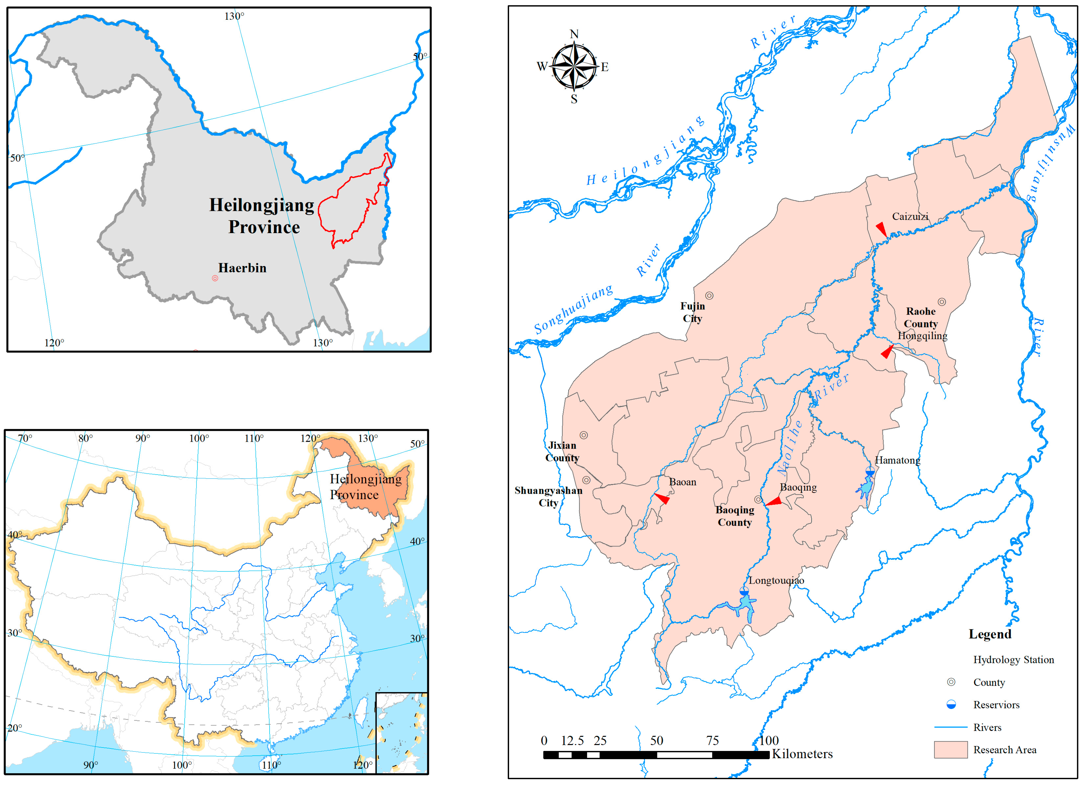
The Naolihe River is located in the east of Heilongjiang Province, China. It is the first tributary of the Wusulijiang River. The Naolihe basin has an area of 24,863 km2 with an elongated shape. The average basin length is about 270 km, and the average width is about 90 km. The ratio of length to width is 3:1. The Naolihe basin lies in the temperate continental monsoon climate zone. The multiyear average precipitation is 545 mm, and 70% of the precipitation is mostly concentrated in June, July, August, and September. Moreover, the precipitation in July and August accounts for about 44% of the total. The precipitation in May and June only accounts for 23%.
Four hydrological stations are present in the Naolihe basin: Baoqing, Baoan, Caizuizi, and Hongqiling, as shown in Figure 1. The Baoqing hydrological station is located in the town of Baoqing, with a drainage area of 3689 km2. The Caizuizi hydrological station is located at the trunk stream of Naolihe River, in the town of Sanlitun, and has a control area of 20,896 km2. The Baoan hydrological station is located in the town of Youyi, having a drainage area of 1344 km2. The Hongqiling hydrological station is located on the Hongqiling farm. Its drainage area is 1147 km2. Two leading reservoirs are found in the Naolihe basin: the Longtouqiao Reservoir and the Hamatong Reservoir, shown in Figure 1. The first reclamation in the Naolihe basin began in 1956, and no agricultural activities were performed in the study area prior to 1956. Therefore, 1956 was chosen as the start year for this study. The historical daily flow data, except for December to March in the next year due to the freezing period, is from 1956 to 2012 for the four hydrological stations in the Naolihe Basin for this study. Location of the study area is shown in Figure 1.
2.2. Methodology
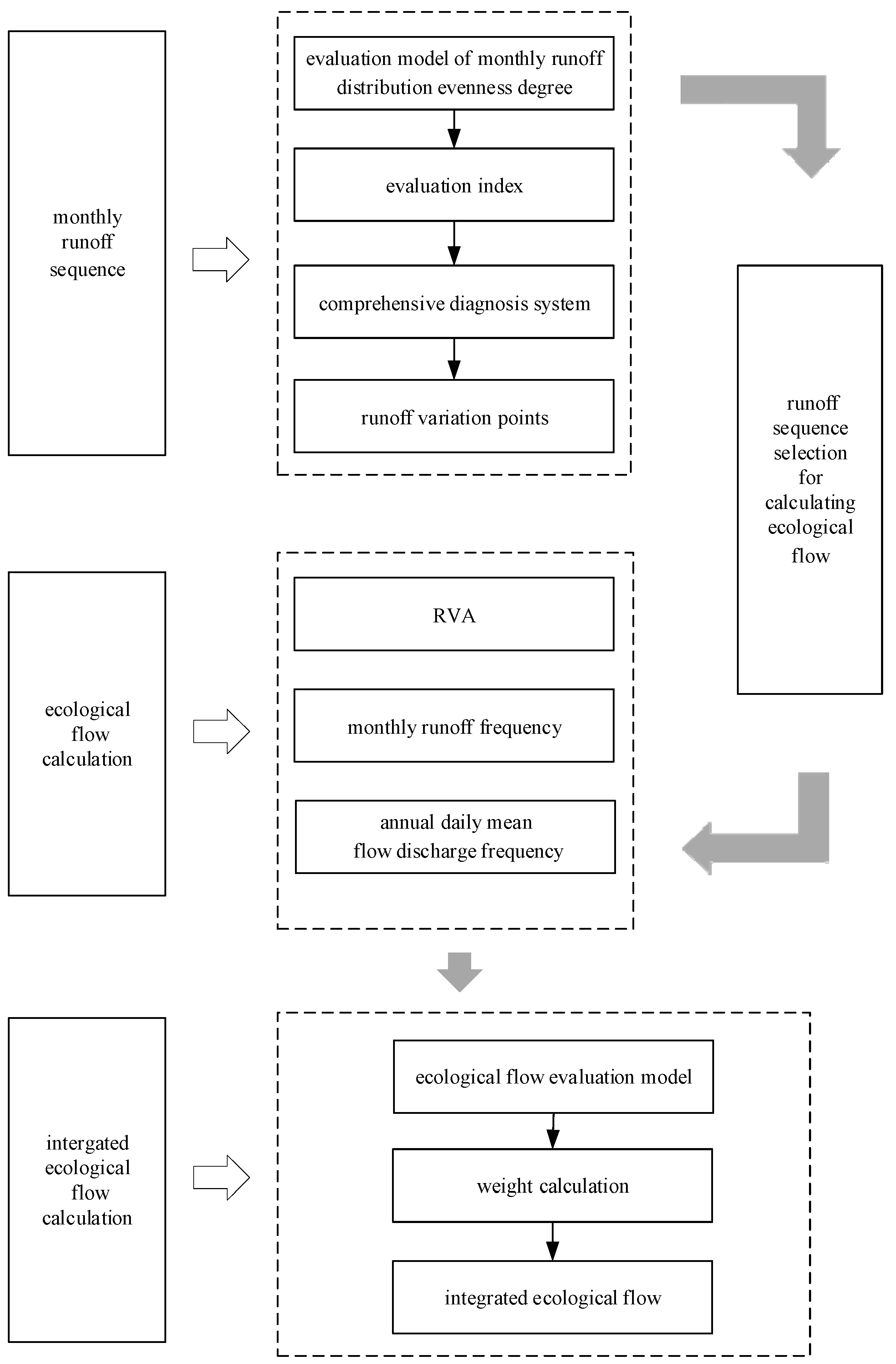
The comprehensive ecological flow was calculated using the weighting mean method. The flow chart of the study process is shown in Figure 2.
2.2.1. Evaluation of the Intra-Annual Runoff Distribution Degrees of Evenness
The Gini coefficient is an index used to quantify and evaluate the degrees of distribution evenness. In this paper, it is used to evaluate intra-annual runoff distribution evenness degrees. The GI of runoff series is calculated as follows:
- (1)
- Group and sort historical monthly flow data. Divide the 12 monthly flows in the ith year into a group, and sort the monthly flows into a group in ascending order. The ascending runoff series of the ith year is , where i represents the ith year, .
- (2)
- Accumulate the ascending runoff data in each group:where k is the ranking order.
- (3)
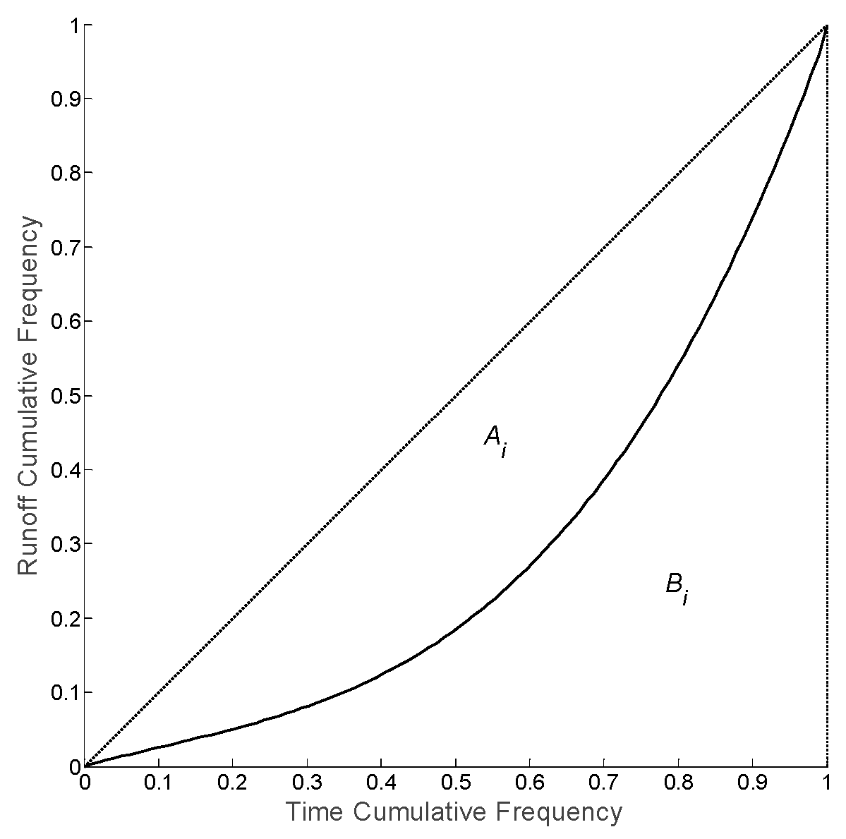
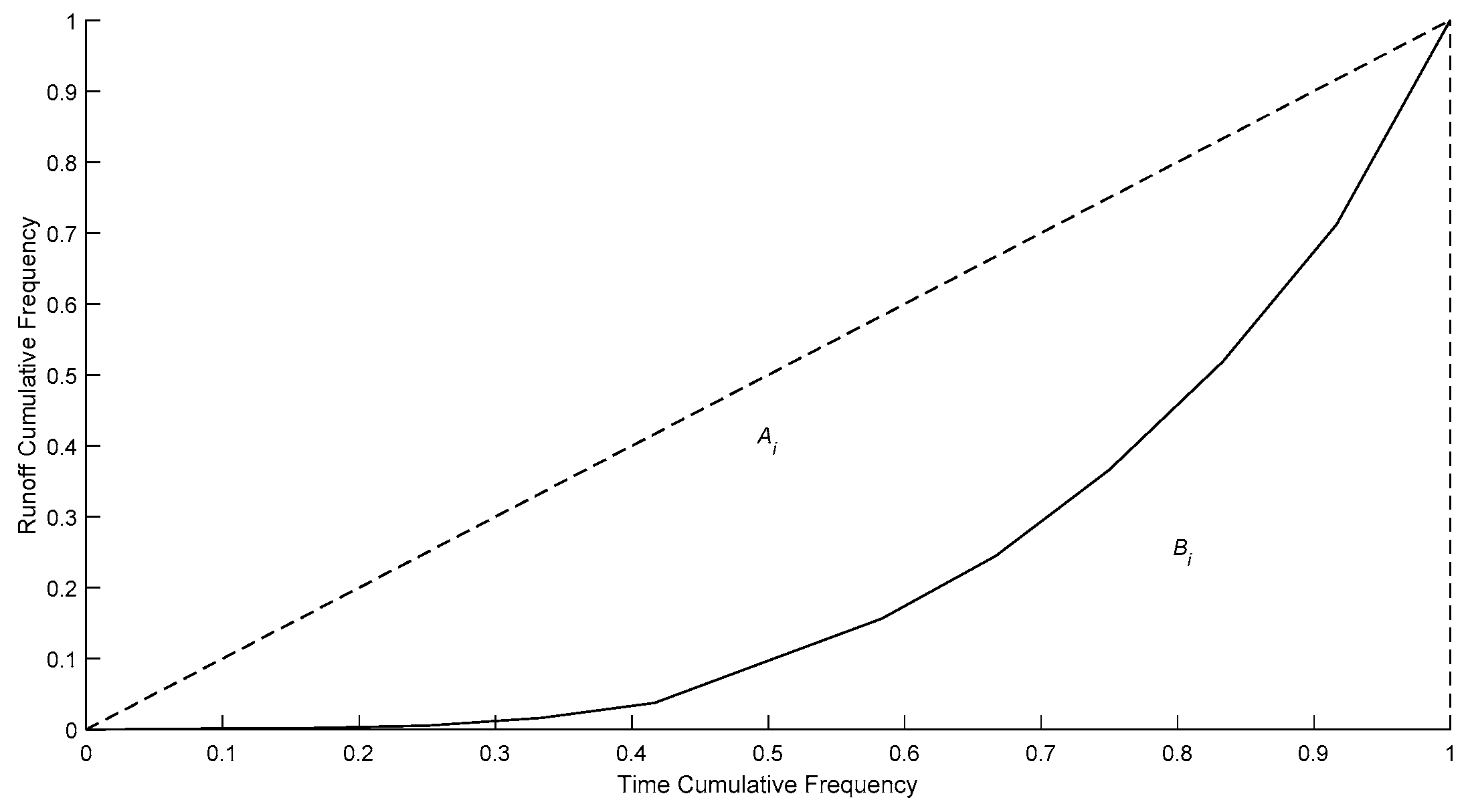
- Draw a Lorenz curve of the annual distribution for monthly flow. Take k/12 as the abscissa, as the ordinate, and draw a Lorenz curve of the annual distribution for monthly flow. The Lorenz curve is shown in Figure 3.
- (4)
- The ith year runoff Gini coefficient GIi is computed as:where SAi and SBi are the area acreages of Ai and Bi, respectively.
The calculation details of GI series in each station are shown in Appendix A.
The smaller the obtained value, the more even the runoff distribution in a year. Conversely, the larger the obtained value, the more uneven the runoff distribution in a year.
2.2.2. Hydrological Alteration Diagnosis System
A single hydrological alteration diagnosis method occasionally produces unreliable results, and multiple hydrological alteration diagnosis methods produce different results. The hydrological alteration diagnosis system synthetically considers the diagnosis results from multiple diagnosis methods and examines the alteration form and alteration point holistically. The steps we followed for alteration diagnosis are as follows. Firstly, we used the Hurst coefficient [25] method and the moving average method to form a primary diagnosis and judge whether or not the series contains an alteration. If so, then various examination methods were used to conduct a detailed diagnosis, including three trend diagnosis methods (the correlation coefficient method, Spearman rank correlation method, and Kendall rank correlation method) and 11 jump diagnosis methods (the Lee–Heghinan method, rank test, slide F test, R/S method, Mann–Kendall method, Bayesian method, etc.). The diagnosis results were also classified into two types, trend results and jump results, and the results were synthesized. Finally, efficiency coefficients were calculated for identifying the alteration form, and the alteration form was judged to determine if one coefficient was bigger than the other one.
2.2.3. Ecological Flow Calculation Method
- In the range of the variability approach (RVA) method, ecological flow calculations should consider the hydrological regime. Parameters of the indicators of the hydrologic alteration (IHA) method are all closely related to runoff, and monthly flow influences river-living organisms, soil, etc. Therefore, the RVA analyses the monthly flow frequency distribution of each month and selects the flow corresponding to 25% and 75% in the frequency distribution as the upper and lower limits of the monthly flow, respectively [26]. Ecological flow is calculated as:where is the ecological flow of the jth month, is monthly mean flow of the jth month, is the upper limit of RVA, and is the lower limit of RVA.
- The steps for ecological flow calculation using the monthly frequency method (MFM) are as follows:
- (1)
- Calculate the monthly flow distribution empirical frequency of the jth month.
- (2)
- Select the probability distribution function and draw the monthly flow distribution theoretical frequency curve of the jth month. The Pearson III distribution curve and generalized extreme value (GEV) distribution curve are commonly used. The GEV distribution curve is better fitting with the runoff data [27].
- (3)
- Select the flow corresponding to the maximum frequency in the GEV distribution curve as the ecological flow of the jth month [28].
- The annual daily mean flow frequency method (ADMFFM) assumes that daily flow may appear in a month with a certain probability. The frequency of daily flow in the jth month of the historical runoff series is calculated and the daily flow corresponding to 60% is selected as the ecological flow [24] of the jth month, . The ecological flow calculated using this method meets the ecological water requirements in different cases.
- In the comprehensive ecological flow calculation method, ecological flow maintains riverine ecological function. Too much or too little will affect the riverine ecosystem. Therefore, the weights of each ecological flow calculation method are used to comprehensively calculate ecological flow. The steps for this method are as follows:
- (1)
- Evaluate ecological flows from RVA, MFM, and ADMFFM, and the comprehensive evaluation values of RVA, MFM, and ADMFFM of the jth month are , and , respectively.
- (2)
- Calculate the comprehensive ecological flow of the jth month as follows:
2.2.4. Weight Calculation of Comprehensive Ecological Flow
The three evaluation indexes listed in Section 2.2.4 were used to evaluate the calculation results following the above ecological flow calculation methods. Three single evaluation results were synthesized into a comprehensive evaluation result. The weights of each single ecological flow calculation result were obtained. The detailed calculation steps are as follows.
- We first determined the deviation rate of monthly flow. The median of the natural daily mean flow series in the jth month of N years was called the standard value. This index is a ratio of ecological flow in the jth month to the standard value. It reflects the deviation degree between the ecological flow and the natural flow in the same period [28,29]. It is computed as follows:
- (1)
- Calculate the natural daily mean flow in the jth month of N years , where i is the year, i = 1, 2, …, N; N is equal to the length of the runoff series; and j is the month, j = 1, 2, …, 12;
- (2)
- Sort in the ascending order , (, n is the serial order), where the standard value of the jth month is ;
- (3)
- The calculation formula of the deviation rate of the monthly flow is:where is the deviation rate of the monthly flow of the jth month and is the ecological flow of the jth month, in m3/s. If the value is close to 1, the calculated flow is approaching the natural flow and the riverine ecosystem is healthy.
- Satisfaction degree of the monthly ecological flow. This a ratio of the days where the natural flow is equal to or greater than the ecological flow to the total number of days in the same month. The formula to calculate the satisfaction of the monthly ecological water requirement is:where is the satisfaction degree of the monthly ecological flow of the jth month, is the number of days where the natural flow was equal to or greater than the ecological flow in the jth month, is the total number of days in the jth month in N years, is the number of days in the jth month, is the natural daily flow on the kth day of the jth month in the ith year in m3/s, and is the ecological flow of the jth month in m3/s. The greater the satisfaction degree of the monthly ecological flow, the healthier the riverine ecosystem.
- Suitability degree of the monthly ecological flow. The monthly ecological flow discrete coefficient is the sum of the discrete degree between the median and the characteristic extreme value of the ecological flow and natural flow. It reflects the suitability degree between the ecological flow and natural flow in a month.where is the discrete coefficient of the monthly ecological flow in the jth month, is the median of the jth month’s ecological flow of over N years, is the median of the jth month’s natural flow of N years, is the maximum of the jth month’s ecological flow of N years, and is the maximum of the jth month’s natural flow of N years. In the case of being greater than 10, it is considered as completely discrete and the value of is taken as 10.The suitability degree of the monthly ecological flow is computed as:When equals 1, a complete suitableness exists between the ecological flow and natural flow in the jth month; when it equals 0, absolutely no suitableness exists between the ecological flow and natural flow in the jth month.This index reflects the degree of suitability between the total ecological flow requirement and the natural flow in a month. When is 1, the total ecological flow requirement and the natural flow completely match. When is 0, the flow is completely unsuitable. A discrete coefficient greater than 10 can be considered completely discrete and the value of the discrete coefficient is equal to 10.
- Ecological flow comprehensive evaluation. The above indexes compare the ecological flow and natural flow from different aspects. The deviation rate of the monthly flow evaluates the degree and magnitude of deviation between the ecological flow and natural flow. The satisfaction degree of the monthly ecological flow temporally analyses the degree of satisfaction between the ecological flow and natural flow. The suitability degree of the monthly ecological flow evaluates the degree of suitability between the ecological flow and natural flow in discrete degrees. The above three indexes were synthesized into a comprehensive index to evaluate ecological flow in the jth month. The formula for calculating is:where and a value of close to 1 means the calculated ecological flow is approaching the natural flow and the riverine ecosystem is healthy.
- Weight calculation of the comprehensive ecological flow. The geometric mean method was used to calculate the weights for each ecological flow calculation method result.
3. Results
3.1. Hydrological Alteration Diagnosis System
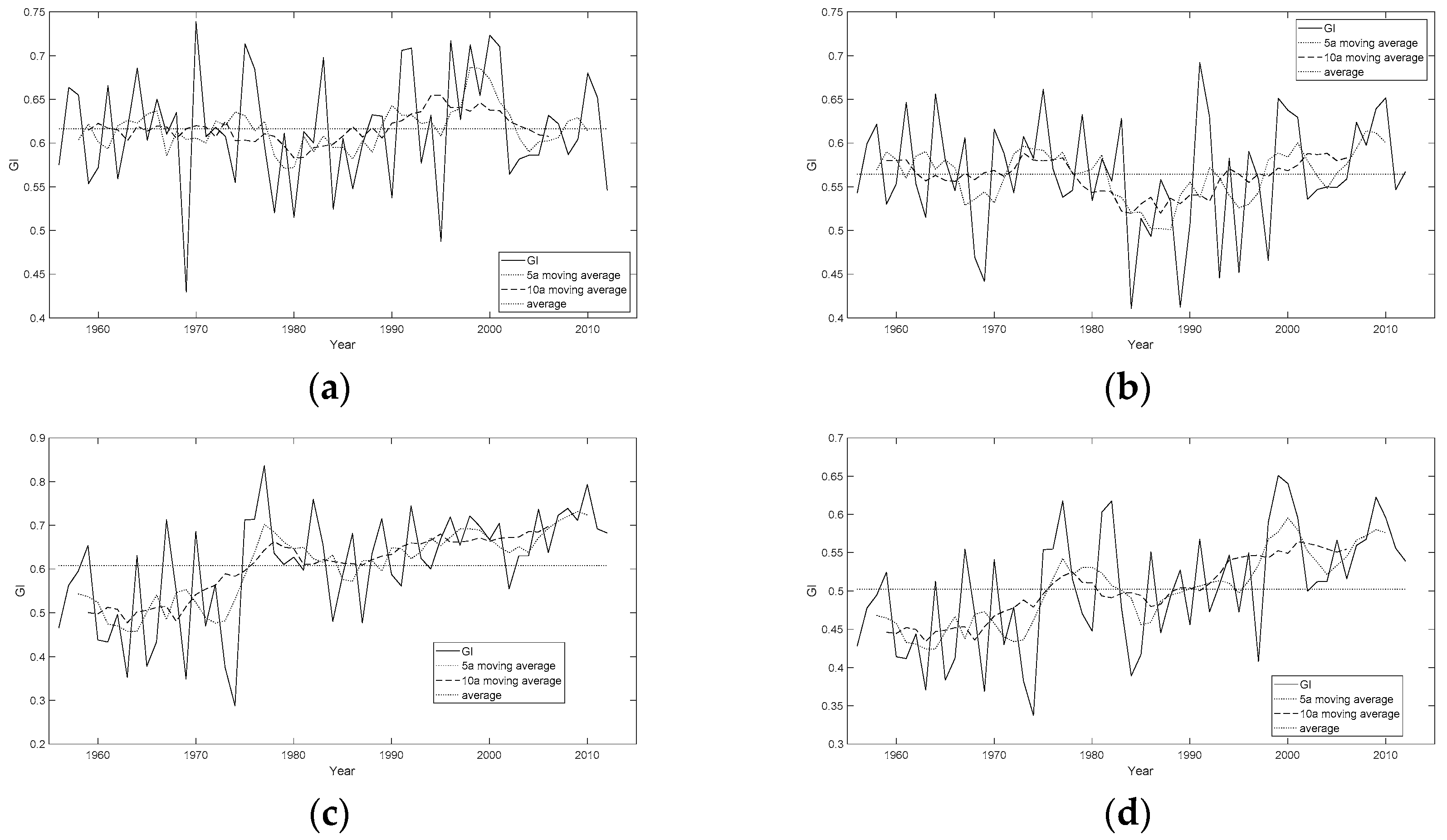
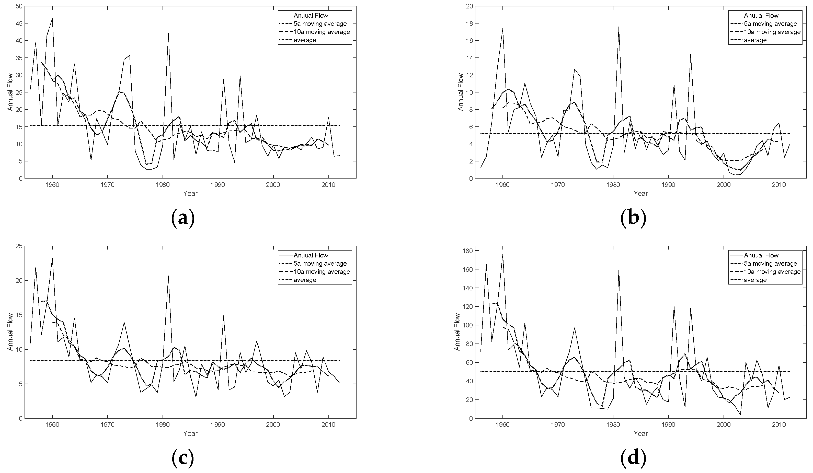
The results of the change in trend in the GI series obtained using the moving average method are shown in Figure 4; the moving average curve for the Hongqiling and Caizuizi stations showed a rising trend. In addition, slight fluctuations were observed in the moving average curves for the Baoqing and Baoan stations. Also, a downward trend exists in the mean annual flow curves shown in Figure 5. Additionally, GI is the index used to quantify and evaluate the evenness degrees of mean annual flow distribution, so there were different trends in GI curves and mean annual flow curves for the same station.
3.2. Results of Ecological Flow Calculation
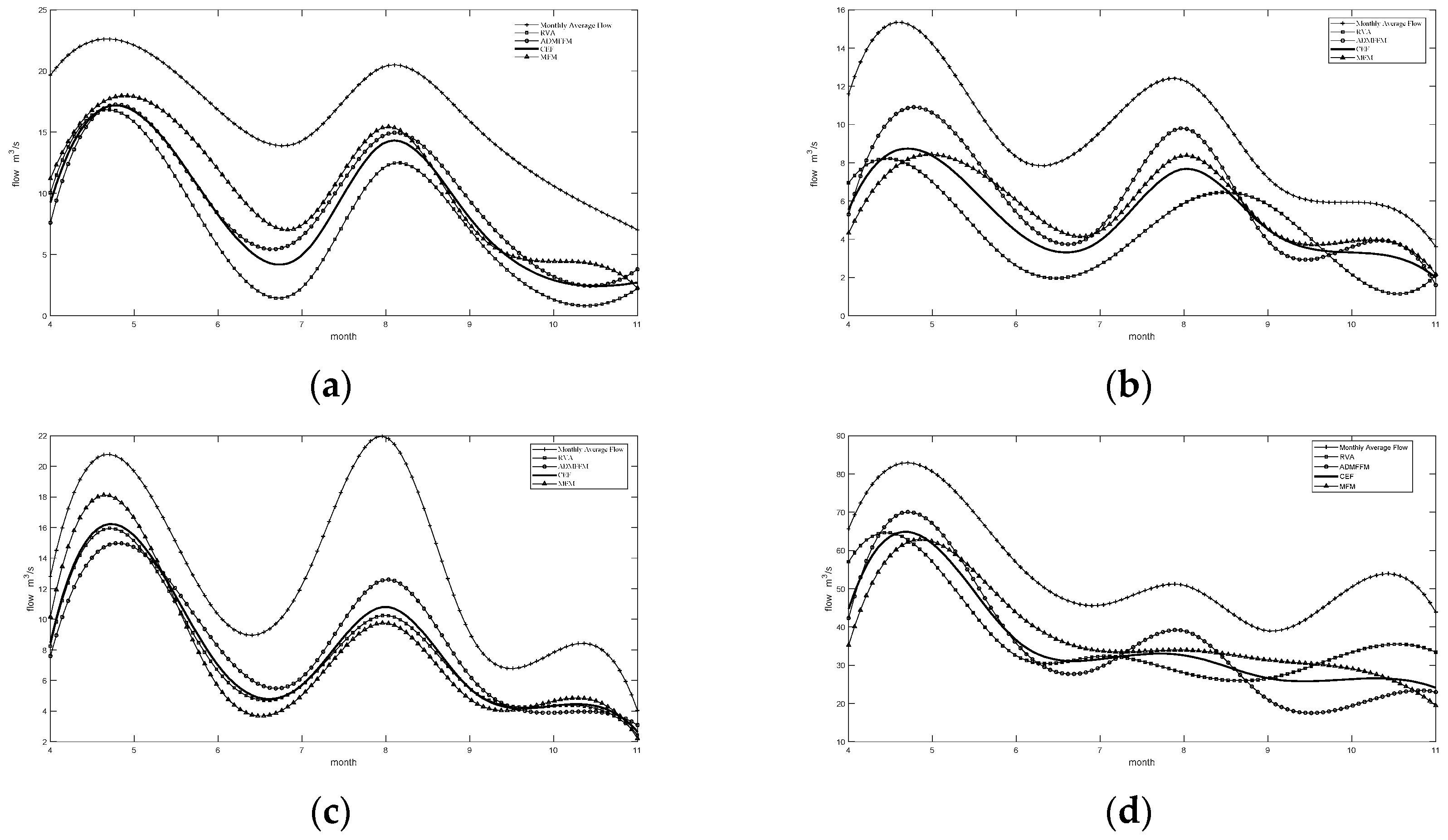
Based on the selected subsequence above, the RVA method, monthly frequency method, and annual daily mean flow frequency method were used to calculate the ecological flows of the four hydrological stations. Comprehensive evaluation results for each method were determined by comprehensive evaluation in Section 2.2.4. The weights of the ecological flow calculated using each method were calculated from comprehensive evaluation results, and the comprehensive ecological flow based on the above methods was obtained. The ecological flows determined using the above methods and their weights are exhibited in Table 2 and Table 3, respectively. The comprehensive ecological flow calculation results are shown in Figure 6.
As shown in Figure 6, comparing the ecological flow values determined by different calculation methods, the ecological flow values from the RVA method were generally low and the ecological flow values from the monthly frequency method were relatively high. However, the comprehensive ecological flow values were all within the extreme values of the three calculation results. The comprehensive ecological flow and the ecological flow obtained from the three methods were all less than the monthly average flow, which is consistent with the characteristics of the ecological flow. In addition, the ecological flow process exactly coincides with the natural flow process, which is shown by the identical timing of extreme ecological flow and extreme natural flow.
The monthly flow meets the ecological water requirements when the monthly flow is greater than the ecological flow, otherwise the ecological water requirement is not satisfied, which means the riverine ecosystem may be damaged. The ecological water requirement damage frequency is a ratio of the number of times the monthly flow was less than the ecological flow to the series length. The calculation results of the ecological water requirement damage frequency of the subsequences and the whole series are shown in Table 4.
4. Discussion
The ecological flow determined using the hydrological method, in which there is no consideration of the effect of some special situations such as overbank flow on the riverine ecosystem, was calculated from historical runoff data. Therefore, the calculated ecological flow regime is in concordance with the natural runoff regime. As the Naolihe basin is located in the cold region of China, precipitation from December to March in the next year is mostly dominated by sleet and solid precipitation involving the formation of snow. The sleet and solid precipitation flow into rivers in the form of snowmelt runoff in April and May in the following year. Flow in April and May accounts for a large proportion of annual flow. Therefore, rivers in the Naolihe basin generally have two flood processes: the spring freshet in April and May and the summer freshet in July and August. As shown in Figure 5, the ecological flow process, which corresponds to the natural flow process, also has two peaks. The maximum peak appears in May, which is consistent with organism reproduction needs in the alpine region.
In Figure 6, the comprehensive ecological flow values were between the values calculated by the three methods. Compared to the bigger values of the three methods, it is can be considered that more water in the river could be utilized for irrigation, drinking, power generation, and so on based on values of the comprehensive ecological flow. At the same time, the water utilization, according to the comprehensive ecological flow, is enough to guarantee the water requirement for the river ecosystem, because they exceed the smaller values calculated by the three methods.
In the Baoqing and Baoan stations, located in the upstream region of the Naolihe river, human activities have relatively little impact on the riverine ecosystem. Therefore, differences in the ecological water requirement damage frequency for the subsequence series and the whole series were not significant. However, the ecological water requirement damage frequency increased obviously in July, August, and September. This is because the study area is located in an agricultural area, and crops need more water in this period. Human use of water resources for irrigation tends to enhance the ecological water requirement damage frequency. However, ecological water requirement damage frequency averages for the subsequence series and the whole series of the Hongqiling station and Caizuizi station were basically the same. This is because the Hongqiling station and Caizuizi station are located in the middle and downstream portions of the Naolihe river, respectively, and the construction of the Longtouqiao and Hamatong Reservoirs effectively solves the problem of instream flow decreasing during the non-flood season. Similarly, during the flood season, due to the impoundment process of reservoirs, part of the natural flow is stored. The instream flow decreases and the ecological water requirement damage frequency increases. In addition, the average ecological water requirement damage frequencies in the Hongqiling station and Caizuizi station were more than in the Baoqing station and Baoan station. This finding is also because of human development.
Author Contributions
Conceptualization, Z.X. and X.G.; Methodology, Y.W., Y.J., J.W.; Validation, Z.X., Y.W., Y.J.; Formal Analysis, Y.W., Z.X.; Investigation, Z.X., Y.W.; Resources, Q.F., Z.X.; Data Curation, Y.W.; Z.X.; Writing-Original Draft, Z.X.; Writing-Review & Editing, Z.X., Y.W.; Visualization, Y.W.; Supervision, X.G., Q.F.; Projection Administration, Z.X., X.G.; Funding Acquisition, X.G.
Funding
This research was funded by the National Key R&D Program of China (No. 2017YFC0406004), the Natural Science Foundation of Heilongjiang province of China (No. E2015024), the Projects for Science and Technology Development of Water Conservancy Bureau in Heilongjiang Province of China (No. 201402, No. 201404, No. 201501), and the Academic Backbones Foundation of Northeast Agricultural University (No. 16XG11).
Acknowledgments
The present study was supported by the Administrative Center for China’s Agenda 21, the Council of Nature Science Funding of Heilongjiang Province, and Water Conservancy Bureau of Heilongjiang Province and Northeast Agricultural University.
Conflicts of Interest
The authors declare no conflicts of interest.
Appendix A. An Example for GI Value Calculation
An example for the GI of the Baoqing station in 1956 is calculated as follows:
The monthly mean flow (monthly flow) series was listed in Table A1.

Table A1.
Historical monthly flow of Baoqing station in 1956.
| Month | 1 | 2 | 3 | 4 | 5 | 6 | 7 | 8 | 9 | 10 | 11 | 12 |
|---|---|---|---|---|---|---|---|---|---|---|---|---|
| Monthly mean flow | 0.08 | 0.009 | 0.027 | 18.4 | 37.7 | 27.4 | 89.5 | 60.1 | 47.5 | 18.6 | 6.6 | 0.57 |
First, sort the monthly flows into a group in ascending order; the result is listed in column (3) in Table A2.
Second, accumulate the ascending monthly flow series by Equation (1); the result is listed in column (4).
Third, calculate the runoff cumulative frequency; for example, 0.000117461 = 0.036/306.486; and calculate the time cumulative frequency; for example, 0.166667 = 2/12.
Fourth, draw a Lorenz curve with the series in column (5) and (6) in Table A2.
Table A2.
Detailed calculation results.
| Month | Order | Monthly Flow | Accumulated Value | Runoff Cumulative Frequency | Time Cumulative Frequency |
|---|---|---|---|---|---|
| (1) | (2) | (3) | (4) | (5) | (6) |
| 2 | 1 | 0.009 | 0.009 | 0.000002965 | 0.083333 |
| 3 | 2 | 0.027 | 0.036 | 0.000117461 | 0.166667 |
| 1 | 3 | 0.08 | 0.116 | 0.000378484 | 0.25 |
| 12 | 4 | 0.57 | 0.686 | 0.002238275 | 0.333333 |
| 11 | 5 | 6.6 | 7.286 | 0.023772701 | 0.416667 |
| 4 | 6 | 18.4 | 25.686 | 0.08380807 | 0.5 |
| 10 | 7 | 18.6 | 44.286 | 0.144495997 | 0.583333 |
| 6 | 8 | 27.4 | 71.686 | 0.233896491 | 0.666667 |
| 5 | 9 | 37.7 | 109.386 | 0.356903741 | 0.75 |
| 9 | 10 | 47.5 | 156.886 | 0.51188635 | 0.833333 |
| 8 | 11 | 60.1 | 216.986 | 0.707980136 | 0.916667 |
| 7 | 12 | 89.5 | 306.486 | 1 | 1 |
Figure A1.
Lorenz curve of the annual distribution for monthly flow in 1956. Note: is a region bounded by Lorenz curve and dashed diagonal, is a region bounded by Lorenz curve and vertical diagonal.
Figure A1.
Lorenz curve of the annual distribution for monthly flow in 1956. Note: is a region bounded by Lorenz curve and dashed diagonal, is a region bounded by Lorenz curve and vertical diagonal.

Then, calculate the areas of and ; the area of is 0.2876 and the sum of the areas of and is 0.5. So, the GI value was calculated by Equation (2), and the result was 0.5752.
The calculation results for each year at the four stations are shown in Table A3.
Table A3.
GI of the four stations.
| Baoqing | Baoan | Caizuizi | Hongqiling | |
|---|---|---|---|---|
| 1956 | 0.575167 | 0.542804 | 0.465529 | 0.428152 |
| 1957 | 0.663721 | 0.599417 | 0.562583 | 0.477699 |
| 1958 | 0.654811 | 0.621435 | 0.5955 | 0.494503 |
| 1959 | 0.553547 | 0.530033 | 0.65446 | 0.524602 |
| 1960 | 0.572132 | 0.553499 | 0.437941 | 0.414069 |
| 1961 | 0.665426 | 0.646424 | 0.43319 | 0.411643 |
| 1962 | 0.559209 | 0.553148 | 0.496531 | 0.443979 |
| 1963 | 0.616581 | 0.515054 | 0.352364 | 0.370382 |
| 1964 | 0.6856 | 0.65623 | 0.630919 | 0.512584 |
| 1965 | 0.603178 | 0.580838 | 0.377696 | 0.383314 |
| 1966 | 0.650194 | 0.545597 | 0.43394 | 0.412027 |
| 1967 | 0.610227 | 0.606012 | 0.713139 | 0.554558 |
| 1968 | 0.634882 | 0.469468 | 0.54839 | 0.470453 |
| 1969 | 0.42967 | 0.441901 | 0.348785 | 0.368555 |
| 1970 | 0.738535 | 0.615852 | 0.686196 | 0.540803 |
| 1971 | 0.607347 | 0.588313 | 0.469413 | 0.430135 |
| 1972 | 0.617986 | 0.543292 | 0.564369 | 0.47861 |
| 1973 | 0.607321 | 0.607421 | 0.375552 | 0.382219 |
| 1974 | 0.555022 | 0.582396 | 0.287487 | 0.337262 |
| 1975 | 0.713496 | 0.661335 | 0.71216 | 0.554058 |
| 1976 | 0.684477 | 0.570556 | 0.713834 | 0.554912 |
| 1977 | 0.595298 | 0.538128 | 0.83657 | 0.617569 |
| 1978 | 0.520268 | 0.545812 | 0.636622 | 0.515496 |
| 1979 | 0.611183 | 0.632446 | 0.61084 | 0.470432 |
| 1980 | 0.515341 | 0.534083 | 0.627068 | 0.44741 |
| 1981 | 0.613004 | 0.581639 | 0.597752 | 0.603207 |
| 1982 | 0.600386 | 0.556539 | 0.759367 | 0.617718 |
| 1983 | 0.697738 | 0.628078 | 0.655349 | 0.477994 |
| 1984 | 0.524324 | 0.410819 | 0.480368 | 0.389041 |
| 1985 | 0.605347 | 0.513835 | 0.584753 | 0.416934 |
| 1986 | 0.547696 | 0.493103 | 0.681788 | 0.551018 |
| 1987 | 0.599018 | 0.558052 | 0.476933 | 0.445092 |
| 1988 | 0.632303 | 0.533406 | 0.635709 | 0.492935 |
| 1989 | 0.630692 | 0.412365 | 0.714885 | 0.527368 |
| 1990 | 0.537402 | 0.507299 | 0.587728 | 0.455828 |
| 1991 | 0.705846 | 0.692314 | 0.561183 | 0.567586 |
| 1992 | 0.708555 | 0.63015 | 0.744296 | 0.472671 |
| 1993 | 0.577032 | 0.445792 | 0.624847 | 0.508258 |
| 1994 | 0.631919 | 0.582762 | 0.600289 | 0.546941 |
| 1995 | 0.487417 | 0.452052 | 0.668352 | 0.472467 |
| 1996 | 0.717055 | 0.590542 | 0.719361 | 0.550217 |
| 1997 | 0.626837 | 0.558618 | 0.6547 | 0.407772 |
| 1998 | 0.712293 | 0.465754 | 0.721465 | 0.589609 |
| 1999 | 0.654239 | 0.651277 | 0.697595 | 0.650854 |
| 2000 | 0.723293 | 0.637565 | 0.667018 | 0.640227 |
| 2001 | 0.710492 | 0.629317 | 0.704367 | 0.595746 |
| 2002 | 0.564298 | 0.535856 | 0.554664 | 0.500066 |
| 2003 | 0.581597 | 0.546915 | 0.630194 | 0.512214 |
| 2004 | 0.585974 | 0.549713 | 0.630597 | 0.51242 |
| 2005 | 0.585971 | 0.549178 | 0.736604 | 0.566536 |
| 2006 | 0.631846 | 0.558946 | 0.637788 | 0.516091 |
| 2007 | 0.621954 | 0.623716 | 0.722809 | 0.559494 |
| 2008 | 0.586923 | 0.597498 | 0.738638 | 0.567575 |
| 2009 | 0.604515 | 0.639023 | 0.71146 | 0.622316 |
| 2010 | 0.680025 | 0.651626 | 0.793393 | 0.595616 |
| 2011 | 0.652022 | 0.546681 | 0.692261 | 0.555792 |
| 2012 | 0.545863 | 0.567307 | 0.683058 | 0.539201 |
References
- Zhang, Q.; Zhang, Z.J.; Shi, P.J.; Singh, V.P.; Gu, X.H. Evaluation of ecological instream flow considering hydrological alterations in the Yellow River basin, China. Glob. Planet. Chang. 2018, 160, 61–74. [Google Scholar] [CrossRef]
- Xia, Z.Q.; Li, Q.F.; Guo, L.D.; Li, J.; Zhang, W.; Wang, H.Q. Computation of minimum and optimal instream ecological flow for the Yiluohe River. IAHS-AISH Publ. 2007, 315, 142–148. [Google Scholar]
- Yang, F.C.; Xia, Z.Q.; Yu, L.L.; Guo, L.D. Calculation and analysis of the instream ecological flow for the Irtysh River. Procedia Eng. 2012, 28, 438–441. [Google Scholar] [CrossRef]
- Xu, Z.X.; Wu, W.; Yu, S.Y. Ecological baseflow: Progress and challenge. J. Hydroelectr. Eng. 2016, 35, 1–11. [Google Scholar] [CrossRef]
- Yang, Z.F.; Cui, B.S.; Liu, J.L. Estimation methods of eco-environmental water requirements: Case study. Sci. China Ser. D Earth Sci. 2005, 48, 1280–1292. [Google Scholar] [CrossRef]
- Chen, M.J.; Feng, H.L.; Wang, L.Q.; Chen, Q.Y. Calculation methods for appropriate ecological flow. Adv. Water Sci. 2007, 18, 745–750. [Google Scholar] [CrossRef]
- Wang, X.Q.; Liu, C.M.; Yang, Z.F. Method of resolving lowest environmental water demands in river course (I)—Theory. Acta Sci. Circumstantiae 2001, 21, 544–547. [Google Scholar] [CrossRef]
- Geoffrey, E.P. Instream flow science for sustainable river management. J. Am. Water Resour. Assoc. 2009, 45, 1071–1086. [Google Scholar] [CrossRef]
- Northern Great Plains Resource Program (NGPRP). Instream Needs Sub-Group Report; Work Group C, Water; US Fish and Wildlife Service, Office of Biological Service: Washington, DC, USA, 1974. [Google Scholar]
- Li, L.J.; Zheng, H.X. Environmental and ecological water consumption of river systems in Haihe-Luanhe basins. Acta Geogr. Sin. 2000, 55, 495–500. [Google Scholar] [CrossRef]
- Yu, L.J.; Xia, Z.Q.; Du, X.S. Connotation of minimum ecological runoff and its calculation method. J. Hehai Univ. (Nat. Sci.) 2004, 32, 18–22. [Google Scholar]
- Ravindra, K.V.; Shankar, M.; Sangeeta, V.; Surendra, K.M. Design flow duration curves for environmental flows estimation in Damodar River Basin, India. Appl. Water Sci. 2017, 7, 1283–1293. [Google Scholar] [CrossRef]
- Danial, C.; Nassir, E.J. Comparison and regionalization of hydrologically based instream flow. Can. J. Civ. Eng. 1995, 5, 235–246. [Google Scholar] [CrossRef]
- Donald, L.T. Instream flow regimens for fish, wildlife, recreation and related environmental resources. Fish. Mag. 1976, 1, 6–10. [Google Scholar] [CrossRef]
- Brian, D.R.; Jeffrey, B.; Robert, W.; David, P.B. How much water does a river need? Freshw. Biol. 1997, 37, 231–249. [Google Scholar] [CrossRef]
- Li, J.; Xia, Z.Q.; Ma, G.H. A new monthly frequency computation method for instream ecological flow. Acta Ecol. Sin. 2007, 27, 2916–2921. [Google Scholar]
- Zhan, C.S.; Wang, H.X.; Xu, Z.X.; Li, L. Quantitative study on the climate variability and human activities to hydrological response in the Weihe River Basin. In Proceedings of the China Academy of Natural Resources Academic Annual Meeting 2011, Wulumuqi, China, 25 July 2011. [Google Scholar]
- Poff, N.L.; Bledsoe, B.P.; Cuhaciyan, C.O. Hydrologic variation with land use across the contiguous United States: Geomorphic and ecological consequences for stream ecosystems. Geomorphology 2006, 79, 264–285. [Google Scholar] [CrossRef]
- Huang, S.Z.; Chang, J.X.; Huang, Q.; Wang, Y.M.; Chen, Y.T. Calculation of the instream ecological flow of the Wei River based on Hydrological Variation. J. Appl. Math. 2014, 11, 1–9. [Google Scholar] [CrossRef]
- Cai, S.Y.; Lei, X.H.; Meng, X.Y. Ecological flow analysis method based on the comprehensive variation diagnosis of Gini coefficient. J. Intell. Fuzzy Syst. 2018, 34, 1025–1031. [Google Scholar] [CrossRef]
- Xie, P.; Chen, G.C.; Lei, H.F.; Wu, F.Y. Hydrological alteration diagnosis system. J. Hydroelectr. Eng. 2010, 29, 85–91. [Google Scholar]
- Hu, C.X.; Xie, P.; Xu, B.; Chen, G.C.; Liu, X.Y.; Tang, Y.S. Variation analysis method for hydrologic annual distribution homogeneity based on Gini coefficient. A case study of runoff series at Longchun station in Dongjiang river basin. J. Hydroelectr. Eng. 2012, 31, 7–13. [Google Scholar]
- Yang, T.; Zhang, Q.; Chen, Y.D. A spatial assessment of hydrologic alteration caused by dam construction in the middle and lower Yellow River, China. Hydrol. Process. 2008, 24, 262–267. [Google Scholar] [CrossRef]
- Li, Z.Y.; Liu, D.F.; Huang, Q.; Zhang, S.A. Study on the ecological flux of the Ziwu River in Hanjiang River based on several hydrological methods. J. North China Univ. Water Resour. Electr. Power (Nat. Sci. Ed.) 2017, 38, 8–12. [Google Scholar] [CrossRef]
- Xie, P.; Chen, G.C.; Lei, H.F. Hydrological alteration analysis method based on hurst coefficient. J. Basic Sci. Eng. 2009, 17, 32–39. [Google Scholar]
- Liu, G.H.; Zhu, J.X.; Xiong, M.Y.; Wang, D.; Qi, S.H. Assessment of hydrological regime alteration and ecological flow at Meigang station of Xinjiang River. J. China Hydrol. 2016, 26, 51–57. [Google Scholar]
- Li, J.F.; Zhang, Q.; Chen, X.H.; Jiang, T. Study of ecological instream flow in Yellow River, considering the hydrological change. Acta Geogr. Sin. 2011, 66, 99–110. [Google Scholar]
- Zhang, Q.; Cui, Y.; Chen, Y.Q. Evaluation of ecological instream flow of the Pearl River basin. Ecol. Environ. Sci. 2010, 19, 1828–1837. [Google Scholar]
- Halwatura, D.; Najim, M.M.M. Environmental flow assessment—A analysis. J. Environ. Proffessionals Sri Lanka 2014, 3, 1–11. [Google Scholar] [CrossRef]
Figure 1.
Location of the study area.

Figure 2.
Flow chart of the study process. Note: RVA is the range of variability approach method.

Figure 3.
Lorenz curve of annual distribution for monthly flow. Note: is a region bounded by Lorenz curve and dashed diagonal, is a region bounded by Lorenz curve and vertical diagonal.
Figure 3.
Lorenz curve of annual distribution for monthly flow. Note: is a region bounded by Lorenz curve and dashed diagonal, is a region bounded by Lorenz curve and vertical diagonal.

Figure 4.
The values and their moving average of the Gini coefficient (GI) from 1965 to 2012: (a) Baoqing station, (b) Baoan station, (c) Hongqiling station, and (d) Caizuizi station. Note: 5a moving average is a moving average of 5 years, and 10a moving average is a moving average of 10 years.
Figure 4.
The values and their moving average of the Gini coefficient (GI) from 1965 to 2012: (a) Baoqing station, (b) Baoan station, (c) Hongqiling station, and (d) Caizuizi station. Note: 5a moving average is a moving average of 5 years, and 10a moving average is a moving average of 10 years.

Figure 5.
The mean annual flow from 1965 to 2012: (a) Baoqing station, (b) Baoan station, (c) Hongqiling station, and (d) Caizuizi station. The results of the hydrological alteration diagnosis system show a jump alteration in the GI series in 1966 at the Baoqing station, a trend alteration in 1990 in the GI series at the Baoan station, and jump variations in the GI series in 1987 and 1990 at the Hongqiling and Caizuizi stations, respectively. The alteration in the GI series of the Baoqing station occurred in 1966, and no obvious alteration was perceived in the GI series in the subsequent 46 years. Based on the alteration analysis above, runoff data from 1966 to 2012 were selected as the subsequence to calculate ecological flow at the Baoqing station. Runoff data for the periods 1956–1990, 1956–1987, and 1956–1990 were selected as the subsequence to calculate ecological flow at the Baoan, Hongqiling, and Caizuizi stations, respectively. Results of the hydrological alteration diagnosis system are shown in Table 1.

Figure 6.
Ecological flow calculation results: (a) Baoqing, (b) Baoan, (c) Hongqiling, and (d) Caizuizi stations.
Figure 6.
Ecological flow calculation results: (a) Baoqing, (b) Baoan, (c) Hongqiling, and (d) Caizuizi stations.

Table 1.
Results of the hydrological variation diagnosis system.
| Diagnosis Method | Intra-Annual Runoff Distribution of GI (1956–2012) | |||||
|---|---|---|---|---|---|---|
| Station | ||||||
| Baoqing | Baoan | Hongqiling | Caizuizi | |||
| Primary diagnosis | Hurst coefficient | 0.741 | 0.896 | 0.727 | 0.615 | |
| Alteration existence | Yes | Yes | Yes | Yes | ||
| Detailed diagnosis | Jump diagnosis | Sliding F test | 1966 (+) | 1990 (+) | 1987 (−) | 1990 (−) |
| Sliding T test | 1966 (−) | 1998 (−) | 2009 (−) | 1981 (+) | ||
| Lee–Heghinan method | 1966 (+) | 1990 (+) | 1989 (+) | 1990 (+) | ||
| Orderly cluster method | 1966 (+) | 1974 (−) | 1987 (+) | 1990 (−) | ||
| R/S | 1989 (+) | 1990 (−) | 1979 (−) | 1990 (+) | ||
| Brown–Forsythe | 1964(−) | 1990(+) | 1987(+) | 1992 (−) | ||
| Sliding run test method | 1992 (+) | 1990 (−) | 1992 (+) | 1985(+) | ||
| Sliding rank test method | 1985 (+) | 1992 (+) | 1987 (+) | 1991 (+) | ||
| Optimum information dichotomy | 1966 (−) | 1989 (+) | 1989 (−) | 1990 (+) | ||
| Mann–Kendall | 1992 (+) | 1992 (−) | 1987 (−) | 1991 (−) | ||
| BSYES | 1966 (+) | 1989 (−) | 1987 (+) | 1989 (+) | ||
| Trend diagnosis | Trend alteration degree | Significant alteration | Significant alteration | Significant alteration | Significant alteration | |
| Correlation coefficient method | (+) | (+) | (+) | (+) | ||
| Spearman | (+) | (+) | (−) | (+) | ||
| Kendall | (+) | (+) | (+) | (+) | ||
| Jump point | 1966 | 1990 | 1987 | 1990 | ||
| Jump | Comprehensive weight | 0.55 | 0.67 | 0.42 | 0.34 | |
| Comprehensive significance | 4 (+) | 5 (+) | 4 (+) | 4 (+) | ||
| Trend | Comprehensive significance | 3 (+) | 3 (+) | 2 (−) | 3 (+) | |
| Comprehensive diagnosis | Alteration form selection | Jump efficiency coefficient/% | 45.3 | 35.1 | 52.5 | 50.3 |
| Trend efficiency coefficient/% | 38.3 | 46.2 | 39.1 | 37.5 | ||
| Diagnosis result | 1966 | 1990 | 1987 | 1990 | ||
Note: + in the table represents a strong alteration, and − represents a weak alteration. The runoff series was altered when the Hurst coefficient was not equal to 0.5 [25].
Table 2.
Ecological flow of the selected series and the whole series in the four stations in the Naolihe basin (m3/s).
Table 2.
Ecological flow of the selected series and the whole series in the four stations in the Naolihe basin (m3/s).
| Station | Method | April | May | June | July | ||||
| (1) | (2) | (1) | (2) | (1) | (2) | (1) | (2) | ||
| Baoqing | RVA | 10.05 | 6.89 | 15.81 | 11.48 | 5.67 | 6.80 | 2.29 | 1.28 |
| MFM | 11.19 | 6.85 | 17.99 | 12.85 | 11.95 | 7.72 | 7.39 | 4.95 | |
| ADMFFM | 7.64 | 5.90 | 16.84 | 12.55 | 8.35 | 6.55 | 6.52 | 4.35 | |
| Baoan | RVA | 6.95 | 4.92 | 6.98 | 4.94 | 2.61 | 1.12 | 2.68 | 1.15 |
| MFM | 4.32 | 3.63 | 8.43 | 6.02 | 6.03 | 4.44 | 4.42 | 3.36 | |
| ADMFFM | 5.32 | 4.92 | 6.98 | 5.44 | 2.61 | 2.94 | 2.68 | 2.54 | |
| Hongqiling | RVA | 8.26 | 8.61 | 15.11 | 12.53 | 6.61 | 3.35 | 5.69 | 0.75 |
| MFM | 10.17 | 9.18 | 16.59 | 12.94 | 5.62 | 5.39 | 5.04 | 3.82 | |
| ADMFFM | 7.61 | 7.60 | 14.72 | 11.7 | 8.21 | 6.35 | 6.21 | 4.70 | |
| Caizuizi | RVA | 57.08 | 37.18 | 30.13 | 38.18 | 30.10 | 32.47 | 17.44 | 29.62 |
| MFM | 35.28 | 34.94 | 62.39 | 55.30 | 43.69 | 39.44 | 33.76 | 30.13 | |
| ADMFFM | 42.31 | 38.65 | 67.89 | 56 | 35.74 | 31.85 | 29.32 | 28.3 | |
| Station | Method | August | September | October | November | ||||
| (1) | (2) | (1) | (2) | (1) | (2) | (1) | (2) | ||
| Baoqing | RVA | 12.21 | 5.14 | 7.02 | 3.25 | 1.32 | 0.49 | 2.22 | 0.98 |
| MFM | 15.42 | 11.66 | 7.44 | 5.09 | 4.44 | 3.01 | 2.26 | 1.63 | |
| ADMFFM | 14.82 | 11.65 | 9.42 | 5.5 | 3.22 | 2.03 | 3.82 | 2.5 | |
| Baoan | RVA | 5.89 | 2.97 | 5.81 | 8.3 | 2.16 | 1.46 | 2.13 | 1.45 |
| MFM | 8.37 | 6.51 | 4.56 | 4.22 | 3.91 | 3.51 | 2.16 | 2.08 | |
| ADMFFM | 5.89 | 5.04 | 5.81 | 5.60 | 2.16 | 2.12 | 2.13 | 1.86 | |
| Hongqiling | RVA | 10.26 | 5.27 | 5.49 | 1.37 | 4.35 | 2.67 | 2.46 | 1.03 |
| MFM | 9.76 | 9.33 | 4.78 | 5.49 | 4.66 | 4.08 | 2.22 | 2.41 | |
| ADMFFM | 12.63 | 11.75 | 6.34 | 5.75 | 3.92 | 3.90 | 3.12 | 2.55 | |
| Caizuizi | RVA | 17.36 | 35.66 | 15.91 | 26.41 | 15.18 | 19.09 | 33.42 | 19.10 |
| MFM | 33.99 | 33.05 | 31.41 | 28.60 | 29.11 | 26.61 | 19.49 | 20.74 | |
| ADMFFM | 39.45 | 37.8 | 21.22 | 22.05 | 19.41 | 22.35 | 23.33 | 22 | |
Note: (1) is the ecological flow calculated by subsequence series selected by the hydrological alteration diagnosis system. (2) is the ecological flow calculated by the whole series. RVA is the range of variability approach method, MFM is monthly frequency method and ADMFFM is annual daily mean flow frequency method.
Table 3.
Weights of ecological flow calculated by RVA, MFM, and ADMFFM based on the subsequence series and the entire series, respectively.
Table 3.
Weights of ecological flow calculated by RVA, MFM, and ADMFFM based on the subsequence series and the entire series, respectively.
| Station | Method | April | May | June | July | ||||
| (1) | (2) | (1) | (2) | (1) | (2) | (1) | (2) | ||
| Baoqing | RVA | 0.31 | 0.29 | 0.44 | 0.32 | 0.44 | 0.31 | 0.42 | 0.32 |
| MFM | 0.25 | 0.35 | 0.32 | 0.43 | 0.30 | 0.40 | 0.24 | 0.42 | |
| ADMFFM | 0.44 | 0.29 | 0.24 | 0.32 | 0.26 | 0.31 | 0.34 | 0.31 | |
| Baoan | RVA | 0.32 | 0.34 | 0.41 | 0.38 | 0.39 | 0.41 | 0.31 | 0.36 |
| MFM | 0.29 | 0.34 | 0.35 | 0.39 | 0.17 | 0.43 | 0.41 | 0.39 | |
| ADMFFM | 0.39 | 0.35 | 0.24 | 0.39 | 0.44 | 0.43 | 0.28 | 0.35 | |
| Hongqiling | RVA | 0.31 | 0.34 | 0.34 | 0.42 | 0.29 | 0.39 | 0.31 | 0.36 |
| MFM | 0.27 | 0.33 | 0.33 | 0.42 | 0.29 | 0.42 | 0.29 | 0.38 | |
| ADMFFM | 0.42 | 0.29 | 0.33 | 0.32 | 0.42 | 0.31 | 0.40 | 0.30 | |
| Caizuizi | RVA | 0.34 | 0.34 | 0.42 | 0.39 | 0.31 | 0.46 | 0.38 | 0.38 |
| MFM | 0.37 | 0.35 | 0.22 | 0.34 | 0.24 | 0.44 | 0.24 | 0.37 | |
| ADMFFM | 0.29 | 0.36 | 0.36 | 0.35 | 0.45 | 0.46 | 0.38 | 0.40 | |
| Station | Method | August | September | October | November | ||||
| (1) | (2) | (1) | (2) | (1) | (2) | (1) | (2) | ||
| Baoqing | RVA | 0.34 | 0.29 | 0.41 | 0.30 | 0.32 | 0.31 | 0.43 | 0.32 |
| MFM | 0.42 | 0.40 | 0.23 | 0.39 | 0.25 | 0.42 | 0.27 | 0.43 | |
| ADMFFM | 0.24 | 0.30 | 0.36 | 0.30 | 0.43 | 0.31 | 0.30 | 0.33 | |
| Baoan | RVA | 0.43 | 0.41 | 0.18 | 0.40 | 0.29 | 0.37 | 0.29 | 0.41 |
| MFM | 0.31 | 0.37 | 0.41 | 0.42 | 0.41 | 0.41 | 0.42 | 0.43 | |
| ADMFFM | 0.26 | 0.38 | 0.41 | 0.41 | 0.30 | 0.39 | 0.29 | 0.43 | |
| Hongqiling | RVA | 0.25 | 0.42 | 0.20 | 0.39 | 0.30 | 0.42 | 0.25 | 0.33 |
| MFM | 0.42 | 0.42 | 0.43 | 0.42 | 0.41 | 0.43 | 0.33 | 0.34 | |
| ADMFFM | 0.33 | 0.31 | 0.37 | 0.31 | 0.29 | 0.31 | 0.42 | 0.30 | |
| Caizuizi | RVA | 0.40 | 0.39 | 0.24 | 0.33 | 0.29 | 0.38 | 0.23 | 0.31 |
| MFM | 0.40 | 0.36 | 0.41 | 0.37 | 0.30 | 0.37 | 0.37 | 0.33 | |
| ADMFFM | 0.20 | 0.37 | 0.35 | 0.36 | 0.41 | 0.40 | 0.40 | 0.38 | |
Note: (1) is the ecological flow calculated by subsequence series selected by the hydrological alteration diagnosis system. (2) is the ecological flow calculated by the whole series. RVA is the range of variability approach method, MFM is monthly frequency method and ADMFFM is annual daily mean flow frequency method.
Table 4.
Ecological water requirement damage frequency in each station (in percent).
| Month | Baoqing | Baoan | Hongqiling | Caizuizi | ||||
|---|---|---|---|---|---|---|---|---|
| (1) | (2) | (1) | (2) | (1) | (2) | (1) | (2) | |
| 4 | 27.26 | 16.89 | 16.14 | 14.67 | 25.86 | 14.57 | 18.12 | 14.61 |
| 5 | 14.63 | 19.35 | 12.23 | 16.57 | 32.43 | 28.07 | 21.86 | 12.87 |
| 6 | 16.15 | 17.29 | 14.97 | 16.12 | 24.79 | 34.65 | 23.44 | 35.32 |
| 7 | 15.89 | 16.23 | 14.03 | 23.87 | 24.68 | 33.74 | 24.34 | 33.47 |
| 8 | 19.55 | 24.56 | 18.10 | 22.48 | 27.65 | 32.80 | 22.80 | 23.49 |
| 9 | 12.56 | 18.96 | 19.57 | 23.63 | 30.08 | 36.36 | 21.42 | 26.31 |
| 10 | 28.65 | 16.23 | 12.18 | 14.35 | 26.79 | 13.57 | 22.62 | 14.06 |
| 11 | 28.63 | 15.99 | 12.70 | 14.30 | 16.36 | 14.73 | 15.98 | 13.04 |
| Average | 20.42 | 18.19 | 14.99 | 18.25 | 26.08 | 26.06 | 21.32 | 21.65 |
Note: (1) is the ecological water requirement damage frequency by subsequence series selected by the hydrological alteration diagnosis system. (2) is the ecological water requirement damage frequency according to the whole series.
© 2018 by the authors. Licensee MDPI, Basel, Switzerland. This article is an open access article distributed under the terms and conditions of the Creative Commons Attribution (CC BY) license (http://creativecommons.org/licenses/by/4.0/).
Share and Cite
MDPI and ACS Style
Xing, Z.; Wang, Y.; Gong, X.; Wu, J.; Ji, Y.; Fu, Q. Calculation of Comprehensive Ecological Flow with Weighted Multiple Methods Considering Hydrological Alteration. Water 2018, 10, 1212. https://doi.org/10.3390/w10091212
AMA Style
Xing Z, Wang Y, Gong X, Wu J, Ji Y, Fu Q. Calculation of Comprehensive Ecological Flow with Weighted Multiple Methods Considering Hydrological Alteration. Water. 2018; 10(9):1212. https://doi.org/10.3390/w10091212
Chicago/Turabian StyleXing, Zhenxiang, Yinan Wang, Xinglong Gong, Jingyan Wu, Yi Ji, and Qiang Fu. 2018. "Calculation of Comprehensive Ecological Flow with Weighted Multiple Methods Considering Hydrological Alteration" Water 10, no. 9: 1212. https://doi.org/10.3390/w10091212
Note that from the first issue of 2016, this journal uses article numbers instead of page numbers. See further details here.