Energy Efficient Operation of Variable Speed Submersible Pumps: Simulation of a Ground Water Well Field

Abstract

Due to their lower energy consumption, permanent magnet synchronous motor (PMSM) submersible pumps have been introduced in ground water well field operation. Besides direct savings of energy, the introduction of PMSM pumps together with the required variable frequency converters offers new operational scenarios to meet the seasonally varying water demand. In this work, potential energy savings of variable speed submersible pumps were investigated. A ground water well field consisting of 13 wells and their transport pipes was modeled in the hydraulic modeling software EPANET 2.0. Using MS visual basic for applications, EPANET was coupled with MS Excel and a genetic algorithm to identify the most energy efficient combination of pump speeds. For the simulated well field, the total specific energy demand required for pumping was significantly lower in partial load operation as compared to nominal pump speed operation. For low and moderate flow scenarios, energy savings in the range of 20% compared to nominal speed operation can be achieved. These findings were confirmed by a monitoring campaign in the well field. Combining hydraulic simulation and optimization using genetic algorithms, the best efficiency scenario for operation of ground water well fields can be found.

1. Introduction

In their efforts to cut greenhouse gas emissions and reduce their fossil energy demand, municipalities often focus on public drinking and wastewater utilities which make up a significant share of municipal energy usage. Approximately 80% of the energy used for drinking water production is required for pumping. If groundwater resources are used, well fields consisting of several parallel submersible pumps are operated to transport groundwater to the drinking water treatment plant. After treatment, the drinking water is stored in tanks and then pumped to the consumers. Whereas optimal energy efficient operation of drinking water distribution networks has been studied intensively [1,2], abstraction and transport of groundwater to the drinking water treatment plant has received considerably less attention. Many studies have been focusing on finding optimal schedules for pumps in water distribution networks, where changes in water demand, electrical tariff and tank level occur in a given time interval. Several authors have proposed mathematical formulations and optimization routines for these multi-objective optimization problems [3,4,5]. In contrast to that, the present study focuses on groundwater abstraction and a simplified modeling approach. Slow changing groundwater levels were assumed to be constant. Compared to drinking water distribution pumps transporting water from a tank in the water treatment plant to the consumer, water demand from groundwater well fields changes seasonally, but shows no variability during the day. Thus, pump switching scenarios are not considered here.

Typically, the seasonally varying drinking water demand implies that the total capacity of a groundwater well field is only needed during a few peak demand days in summer. Thus, the average groundwater abstraction is much lower than the potential total capacity of the well field. Traditionally, in low-demand periods, only a fraction of the wells in a well field is active, i.e., the necessary quantity of water is delivered with adequate pressure by a few fixed-speed submersible pumps. Whereas asynchronous motors (AM) are commonly used in groundwater wells, permanent magnet synchronous motors (PMSM) offer significant higher energy efficiency [6,7,8] but require higher investment as well as rare earth elements in their production. If AM submersible pumps are exchanged against PMSM pumps, significantly lower energy cost result, but additional investment in variable frequency converters and electrical filters is needed. On the other hand, speed control by variable frequency drives offers new operational scenarios to achieve the required target flow in a well field and can reduce the total energy demand.

In this work, the potential energy savings of variable speed PMSM submersible pumps operated in a complete well field were investigated and compared to pumps operated at fixed, nominal speed. Whereas efficiency gains by recent PMSM technology in individual pumps were investigated in another study [6], this study focused on the optimal operation of PMSM pumps in a well field and its benefits. A groundwater well field consisting of 13 submersible pumps was modeled using EPANET 2.0 [9]. After PMSM pumps were selected for each well depending on well productivity, operation of variable speed pumps was simulated. To identify the most energy efficient combination of pump speeds at common operational scenarios, a genetic algorithm was used.

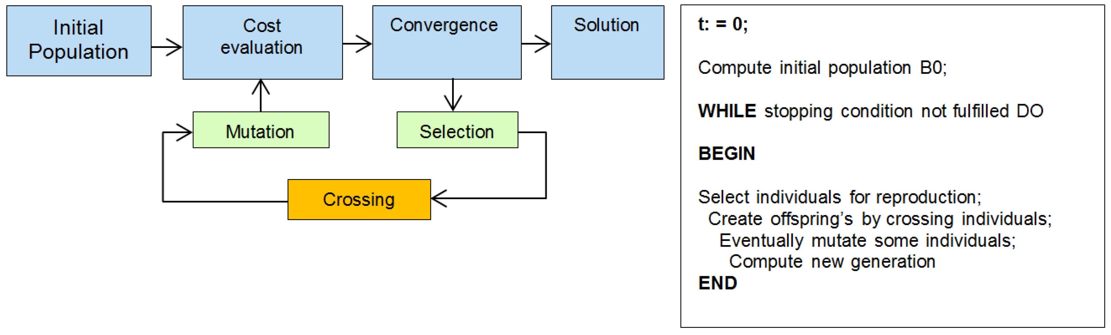
Optimization Using Genetic Algorithms

Genetics algorithms [10] can be considered as computer programs that mimic the process of biological evolution to solve optimization problems. They contain potential solutions in a chromosome-like data structure and apply recombination and mutation operators to preserve critical information. They are also considered as function optimizers, although the range of problems in which they can be implemented is very broad (e.g., optimization of routes/distribution, resources and processes). Their advantages include robustness in addressing multi-objective problems or problems with nonlinear constraints [11]; their ability to optimize variables of different nature, namely continuous and/or discreet values, binary variables and their capacity to process a very large number of variables; their ability to simultaneously sample several portions of a cost surface; and they can be easily adapted to parallel computing and for solving highly complex problems [12].

The operation of these algorithms is based on the following three principles [13].

Evolution is developed at level of chromosomes: organisms do not evolve. They only serve as a container where genes are transported. Nature tends to make more copies of chromosomes that are in better-adjusted organisms: if an organism survives long enough and is healthy, its genes are more likely to pass to the next generation through reproduction. Diversity in the population must be maintained: to ensure variation between organisms, mutations frequently occur. These genetic mutations often result in characteristics that are normally useful for the survival of individuals.

The functioning of these algorithms entails six steps [14,15] (Figure 1):

• Initialization (initial population): An initial population is created. This population is generated, in principle, randomly and can be of the desired size, from a couple of individuals to thousands.
• Cost evaluation (aptitude): Each member of the population is evaluated and the adjustment or aptitude for that individual is calculated. The adjustment value is calculated based on how well the individual are adjusted to the established requirements.
• Selection: This procedure is executed to constantly improve the population. The selection discards bad solutions in a way that keeps the best individuals in the population.
• Crossing: During crossing, new individuals are created by combining aspects of the individuals selected in the previous stage.
• Mutation: It is required to add some randomness to the genetics of the population; otherwise, every combination of solutions that could be created would be in the initial population, that is, it would be trapped in a local optimum.
• Iteration/convergence: Once there is a new generation, the process starts from step two until a stopping criterion is reached.

2. Materials and Methods

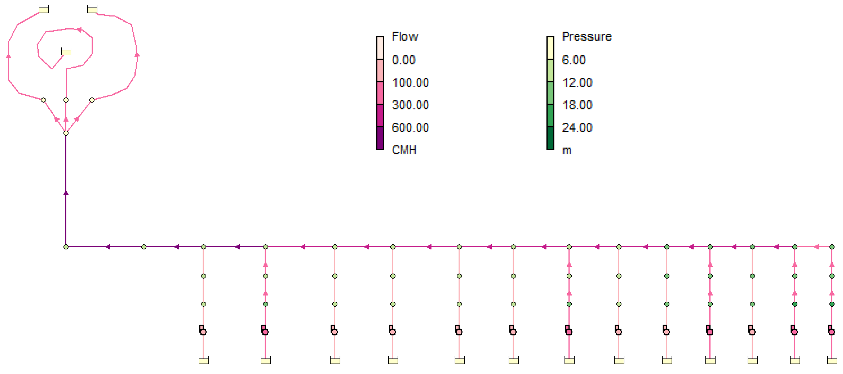
2.1. Hydraulic Modeling of Groundwater Abstraction and Transport

Groundwater abstraction and transport to the drinking water treatment plant is modeled using EPANET 2.0, hydraulic modeling software widely applied to design water distribution networks and optimize their operation [9]. Following an established methodology, groundwater wells and transport pipes are schematized as reservoirs, pumps, pipes and other resistances (fittings, bends, etc.) [17]. In EPANET, these elements are connected by junctions and the total head can be calculated according to Equation (1), in which ∑ h is the sum of friction and minor losses in system (mwc), p is the pressure (N/m²), ρ is the density of the fluid (kg/m³), g is the gravitational constant (m/s²) and z is the elevation (m).

$$z_1+\frac{p_1}{\rho ·g}+\frac{v_1^2}{2g}=z_2+\frac{p_2}{\rho ·g}+\frac{v_2^2}{2g}+{\displaystyle \sum }h$$

(1)

The headloss in pipes can be calculated using the Darcy–Weisbach equation (Equation (2)) from a given length L (m), diameter D (m), the velocity through the pipe v (m/s), the gravity constant g and the roughness coefficient f_D (mm).

$$h_f=f_D·\frac{L}{D}·\frac{v^2}{2g}$$

(2)

Minor head losses through bends and fittings such as valves are described using Equation (3), where K is the minor loss coefficient (-). The EPANET hydraulic solver provides the solution for heads and flows by simultaneously solving the conservation of flow equation for each junction and the headloss equation across each link in the network.

$$h_L=K·\frac{v^2}{2g}$$

(3)

For pump operation at variable speed (n_i), the relationships among flow (Q_i), head (H_i) and power (P_i) at different pump rotational speed can be described by the affinity laws (Equation (4)–(6)).

$$\frac{Q_1}{Q_2}=\frac{n_1}{n_2}$$

(4)

$$\frac{H_1}{H_2}={\left(\frac{n_1}{n_2}\right)}^2$$

(5)

$$\frac{P_1}{P_2}={\left(\frac{n_1}{n_2}\right)}^3$$

(6)

Equation (6) implies that, if the pump speed is reduced, the efficiency curve will be shifted to the left, but the efficiency for n₁ and n₂ will be constant. An alternative relationship has been proposed by Sárbu and Borza [18].

Because EPANET 2.0 power calculation for variable speed pumps are not correct [19,20], power consumption is calculated within MS Excel using the affinity laws and the pump efficiency curves for nominal speed (100%), as shown in Figure 2. For a given set of relative pump speed values, EPANET calculates flow and the corresponding specific energy demand used for pumping is then calculated for each pump within MS Excel using Equation (7), where w_P,i is the specific energy demand needed for pumping and η_i is the efficiency for a submersible well pump i.

$$w_{P,i}=\frac{P_i}{Q_i}=\frac{\rho ·g·H_i}{{\eta }_i}$$

(7)

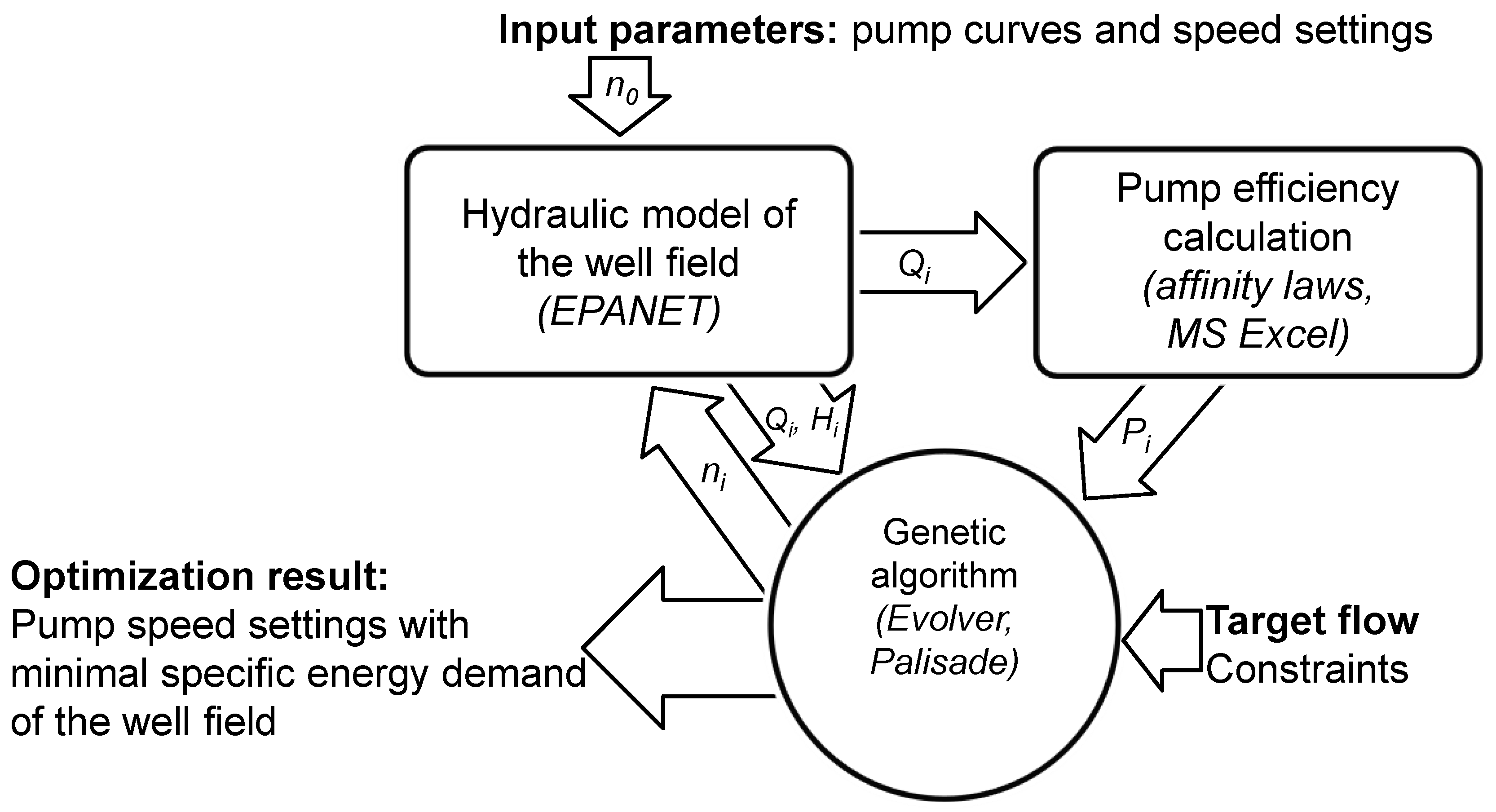
2.2. Optimization Through Genetic Algorithms Using Evolver

To find the optimal combination of pump speed settings, a genetic algorithm is used. The objective is the minimization of the total specific energy demand of the well field, as given by Equation (8).

$$w_{P,total}={\displaystyle \sum }_{i=1}^n{w}_{P,i}$$

(8)

During optimization, the genetic algorithm varies the pump speed and several iterations of EPANET simulations and efficiency calculations are run until a specified stopping criterion is reached. To simulate different operational scenarios, the total flow of the well field is set as a constraint within the optimizer. In addition, for an active pump, a minimal relative pump speed of 70% was set to reduce computing time and because motor efficiency cannot be assumed constant at lower speed values. Thus, all valid scenario calculations consist of a number of active pumps at 70–100% speed and some inactive pumps at speed zero which together produce a specified target flow.

Evolver is an optimization tool add-on designed by the Palisade^® corporation (Ithaca, NY, USA) for Microsoft Excel^® (Redmond, WA, USA) [13]. It allows addressing several optimization problems in a more efficient way in comparison to the default embedded optimization tools in Excel (e.g., Solver). It operates with Genetic Algorithms, and once it is installed in MS Excel, it provides a series of adaptation possibilities. The general idea is to model the problem with all the tools available in MS Excel, including MS Visual Basic for applications (VBA) and then to establish the optimization requirements (number of iterations, initial population, restrictions, objective function, etc.) through the embedded graphical interface provided by Evolver. This offers an easy-to-handle operational framework, which allows the implementation of a heuristic based optimization tool without requiring advanced programming skills.

Before starting the optimization process, one of the first tasks carried out by the algorithm is to run a first tour over the search space to find a feasible solution, in which all the restrictions are met, although the final value adopted by the objective function does not necessarily have to correspond to any optimum (neither global nor local). This option can be deselected by the user. In that case, the algorithm will proceed to the search from a random point. During the execution of the optimization process, the evolution of several optimization parameters can be visualized: number of satisfied restrictions, number of not met restrictions, the objective function result, a graph representative of the degree of diversity existing between the solutions, a graph of evolution of the solution throughout all the iterations, and the adopted values for all the solutions in a generation, among others.

The optimization follows a mono-objective approach, thus, to address multi-objective problems, it is required to carry out a problem generalization, which entails the definition of one of the objectives as objective function and the rest as constrains. In relation to the research field of water supply networks, the Evolver-Excel environment can be connected to the EPANET hydraulic simulation software by means of the EPANET Toolkit [9] to automatically operate the simulation (parameters definition and results extraction) from the above-mentioned environment. In the last five years, it has been used in several works related to optimization of water supply networks [21,22,23,24].

2.3. Case Study: Well Field Tegel-Ost

The Berlin-Tegel waterworks are the oldest and one of the largest of the nine waterworks in Berlin. In the well field Tegel-Ost, eleven wells have been equipped with PMSM submersible pumps, while the two remaining wells are still operated with AM pumps. All wells are equipped with frequency converters to allow for variable speed operation of each pump. Based on the pump curves, elevation and dimension of the wells and pipes, an EPANET model of the well field was developed, which is schematically shown in Figure 3. The 13 wells are represented by reservoirs connected to pumps which feed into riser and connecting pipes and subsequently to the main raw water line to the tower aeration. Each well pump is represented by its individual pump curve, which was measured before installation. The nominal diameter (DN) of the riser and connecting pipes is DN 150 and DN 200, respectively. The main line spans 577 m and expands from DN 300 from the point farthest to the aeration tower to DN 1400 after all 13 wells have been connected. All lengths and diameters of the raw water pipe segments were entered in the model according to their real-world values. The elevation of the main line was set at 33 m ASL (above sea level). The aeration tower is represented by the three reservoirs at 43 m ASL in the upper left of Figure 3. Furthermore, the following simplifications were used in the model:

The dynamic water level in the wells was assumed to be constant at 25 m ASL. The roughness coefficients in the pressure pipes and the minor loss coefficients for the valves were assumed to be equal. Model simulations were run without further calibration and simulation results are expected to deviate from real values. Therefore, a monitoring campaign was set up to compare simulation results to measurements.

2.4. Monitoring Campaign

Typical operational scenarios are defined by statistical analysis of the annual total ground water abstracted in the well field. Based on that, low and moderate flow scenarios were defined. The corresponding pump speed values were set in the waterworks. After waiting 15 min to let the system attain a stable operating state, flow, pressure and power demand were measured and recorded at each well together with the selected pump speed. All wells are equipped with a magnetic flow meter and a manometer which provide flow and pressure data, respectively. Pump speed and power demand were read from the frequency converter.

3. Results and Discussion

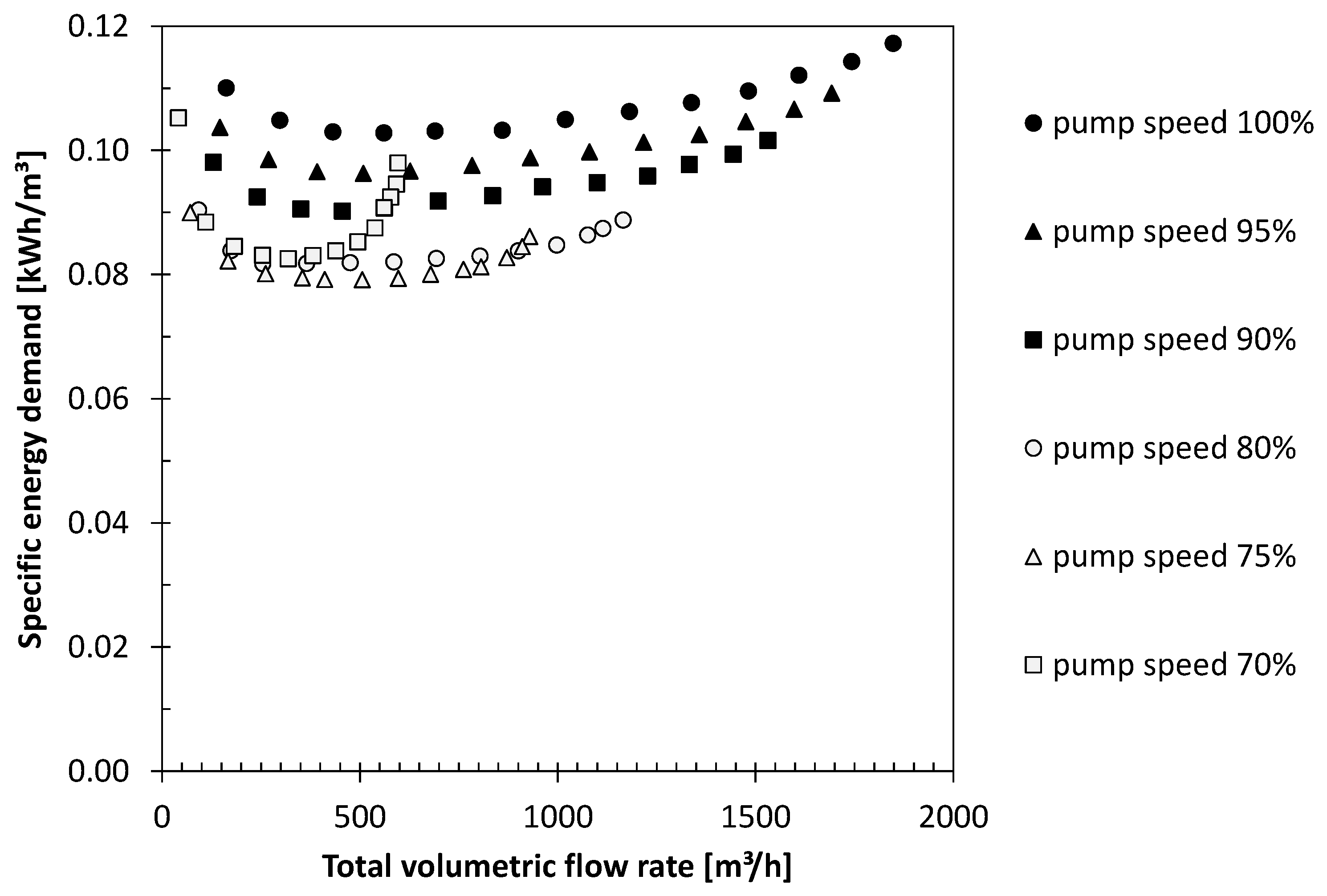
3.1. Simulation of Different Operational Scenarios Using Variable Speed Submersible Pumps in a Well Field

In Figure 4, the resulting total well field flow which can be realized by the 13 pumps in the well field is shown, depending on how many of them are active and on their adjusted speed. On the y-axis, the resulting specific energy demand is shown, which is the sum of the power consumption of each active pump (as given by its efficiency curve) divided by the total well field flow. For each pump speed setting, 13 simulations are shown, beginning with only one active pump corresponding to the lowest well field flow and going up to all 13 pumps in parallel operation. If all 13 well pumps are operated at 100% speed, the simulated flow from the well field amounts to approximately 1850 m³/h, represented by the black dot in the upper right of Figure 4. By gradually turning off the well pumps with the highest specific energy demand, the other points of the upper curve, representing 100% pump speed, are simulated. In all simulations, the last well in the well field remained active to ensure flow through the collection pipe.

Analogously, the specific energy demand and total well field flow was simulated for pump speeds of 95%, 90%, 80%, 75% and 70%. It is clear in Figure 4 that a specific target flow of, e.g., 750 m³/h, can either be realized by five active pumps operating 100% speed or by six pumps at 95% speed, as well as by seven pumps at 80% speed. For well field flows lower than the full capacity, operation of more pumps at reduced speed reduces the specific energy demand required to abstract groundwater and transport it to the water treatment plant, compared to operation of fewer pumps at full speed. For flows lower than 900 m³/h, a pump speed of approximately 75% seems to be optimal, since the simulation of pumps at 70% speed leads to higher specific energy demand.

However, the shape of the curve shown in Figure 4 depends on the chosen pumps. Whereas in this simulation procedure, the pumps with highest specific energy demand were subsequently turned off, a different combination of active well pumps will result in a different relation of specific energy demand to well field flow. In addition, pump speed was manually varied for all pumps in 5% steps, but not individually for each pump. While clearly showing that the optimal operating points are roughly in the range of 75% pump speed, the optimal pump speed combination can only be found by employing an optimization procedure.

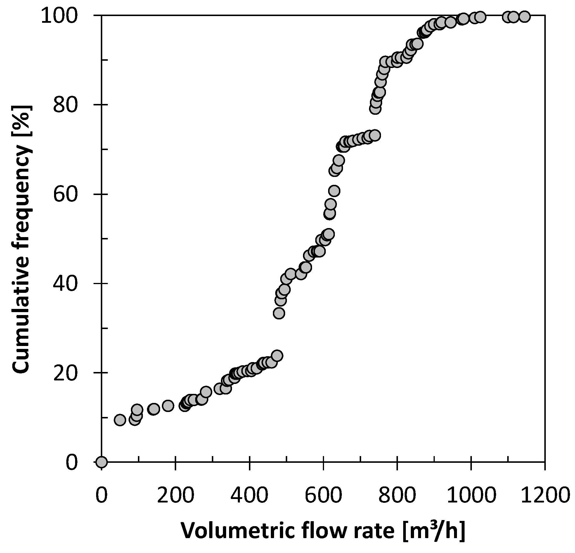
3.2. Analysis of Seasonal Variations in Groundwater Abstraction

Groundwater abstraction varies within a year due to the varying drinking water demand. To define typical operational scenarios, these seasonal variations of groundwater abstraction were analyzed. Figure 5 shows the cumulative frequency of the total volumetric flow in the well field. Whereas the maximum flow of abstracted groundwater is approximately 1100 m³/h, the median flow amounts to only 600 m³/h. Based on these data, a typical low load scenario was defined corresponding to a total volumetric flow of 430 m³/h. Accordingly, the moderate flow scenario corresponds to a total volumetric flow rate of 740 m³/h.

3.3. Simulation of Typical Operational Scenarios and Optimal Pump Speed

For the defined scenarios, an optimal combination of pump speeds was determined using the genetic optimization algorithm and the EPANET model of the well field.

Table 1. Pump speed settings and simulation results for total well field flow and specific energy demand for low and moderate flow scenarios.

	Low Flow Scenario				Moderate Flow Scenario
	Nominal Speed		Variable Speed		Nominal Speed		Variable Speed
Pump	Pump Speed (rpm)	Pump Speed (%)	Pump Speed (rpm)	Pump Speed (%)	Pump Speed (rpm)	Pump Speed (%)	Pump Speed (rpm)	Pump Speed (%)
1	3000	100	2250	75	-	-	2280	76
2			2160	72	3000	100	2190	73
3			2130	71			2190	73
4	3000	100
5							2220	74
6			2130	71			2280	76
7					2850	100
8							2220	74
9			2160	72			2220	74
10					3000	100
11
12					3000	100	2250	75
13	2850	100	2052	72	2850	100	2109	74
Total well field flow (m3/h)	432		432		744		740
Specific energy (kWh/m3)	0.10		0.08		0.11		0.08

shows EPANET simulation results for: (a) a manually chosen well pump setup to reach the required flow rate with pumps at 100% speed; and (b) for the optimal pump speed setting suggested by the optimization routine. The simulated total well field flow rates are very similar and close to the target of 430 m³/h and 740 m³/h, respectively. The specific energy demand in the reduced pump speed scenario is 0.08 kWh/m³ in both the low flow and the moderate flow scenario. In both cases, the specific energy demand in the reduced pump speed scenario is significantly lower than in the scenarios with 100% pump speed. The pump speed settings determined by the optimization procedure are very close to the roughly estimated optimal pump speed of approximately 75% (cf. Section 3.1) and confirm these results.

The significant increase in energy efficiency can be explained by analysis of the pump operating points. Figure 6 shows the pump curves of (Figure 6a) Well Pump 1 in the low flow scenario and (Figure 6b) Well Pump 2 in the moderate flow scenario as well as the corresponding efficiency curves (Figure 6c,d). The pump and efficiency curves at 75% (low flow) and 73% (moderate flow) pump speed have been calculated using the affinity laws (Equation (4)–(6)). The operating point is determined using the EPANET simulated flow. As can be seen in Figure 6, the operating point shifts from the right side of the pump curve to the center of the pump curve. For Well Pump 1, the volumetric flow in the low flow scenario is reduced from 135 m³/h to 56 m³/h, the head decreases from 22.7 mwc to 18.8 mwc. On the efficiency curve, the operating point is shifted closer to the optimum, resulting in an efficiency increase from 59.6% to 65.4%. In the moderate flow scenario, a very similar behavior can be observed. At 100% pump speed, the operating point is to the right of the last point of the efficiency curve, resulting in a non-optimal efficiency. In the reduced speed scenario, flow is reduced from 172 m³/h to 87 m³/h and the head from 25.9 mwc (meter of water column) to 20.2 mwc. The efficiency is shifted from 63.9% right to its optimum of 70.4%. This illustrates that, for low and moderate loads, the chosen pumps in the well field will operate out of their optimal range if operated at 100% speed. Instead, lower speed settings lead to optimal efficiency.

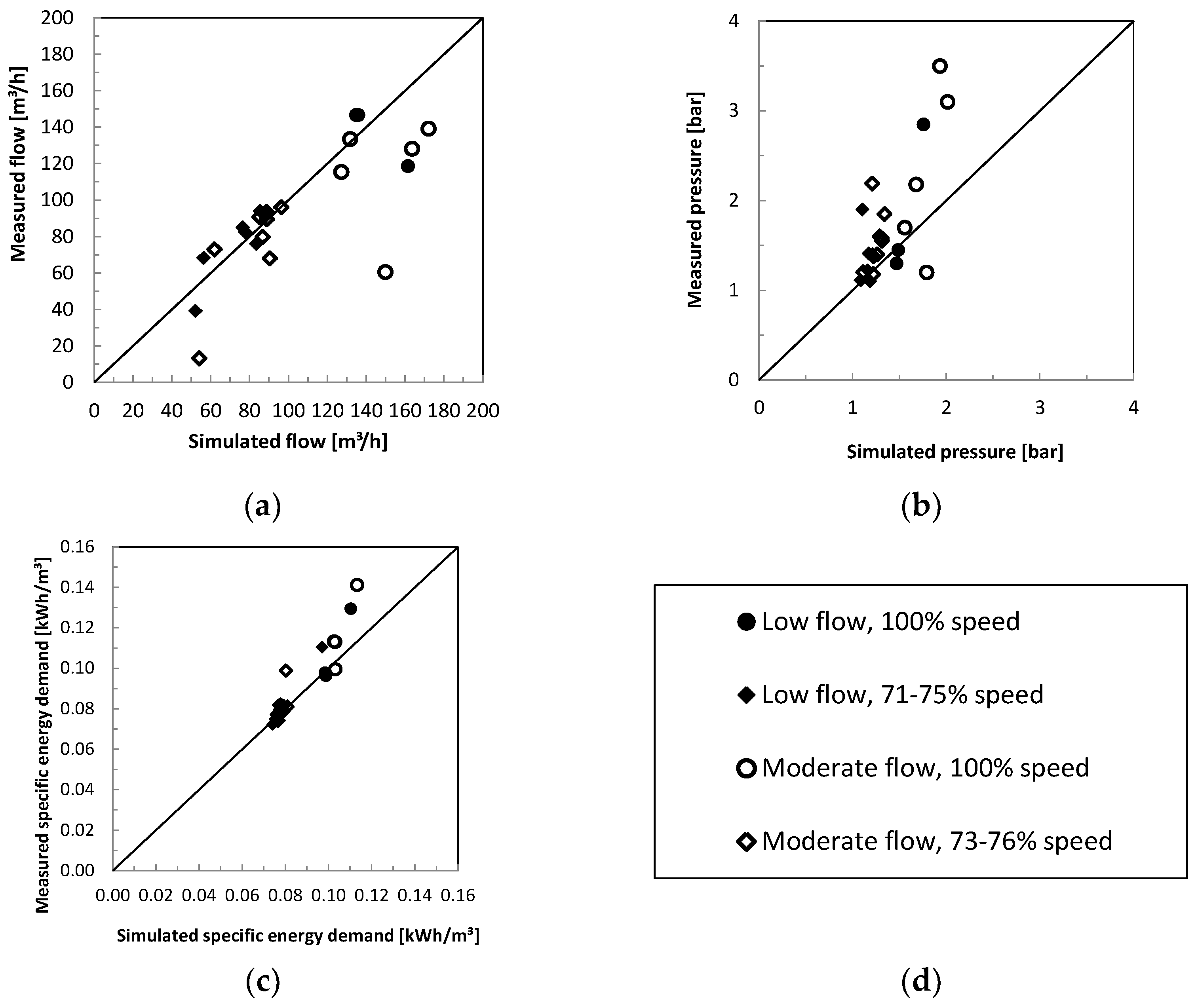
3.4. Comparison of Simulation and Measurements

Given the mentioned simplifications and shortcomings of the model, the simulations are expected to deviate more or less strongly from measurements. Figure 7 shows measured and simulated (Figure 7a) volumetric flow, (Figure 7b) head and (Figure 7c) specific energy demand of the well pumps for the low and moderate well field flow scenarios described above. At 100% pump speed, some of the measured flow values are significantly lower than simulated. At reduced pump speed, the deviations seem to be smaller. In several wells, measured head is approximately 1–2 bar higher than simulated, especially at 100% pump speed, whereas less deviation can be seen at reduced pump speed. This clearly shows that local head loss is not correctly simulated in all of the wells. This could be due to lower dynamic water levels in the well, but also by locally higher head losses caused by iron ochre formation, which is not accounted for in the model. Figure 7c shows that the measured specific energy demand correlates fairly well with the simulated values, although measured values are generally higher. The measured mean specific energy demand of the well field at 100% pump speed amounts to 0.11 kWh/m³ as compared to the simulated value of 0.10 kWh/m³. At reduced pump speed, the measured and simulated specific energy demand have the same value of 0.08 kWh/m³. For the low flow scenario, the lower energy demand at reduced pump speeds as compared to 100% pump speed corresponds to potential savings of 20%. In the moderate flow scenario, the measured mean specific energy demand of 0.13 kWh/m³ at 100% pump speed is higher than the simulated value of 0.11 kWh/m³. At reduced pump speed, the measured mean specific energy demand is 0.09 kWh/m³, slightly higher than the simulated value of 0.08 kWh/m³. Based on the measured data, the saving potential is approximately 31%.

Although model simulations could not exactly meet the measured values, the specific energy demand required for pumping is reduced in the same range if pump speed is reduced. The observed discrepancies may be caused by the earlier described model simplifications and model accuracy may be improved by finer calibration. The calculated saving potential of optimized reduced speed operation compared to pumped operation at nominal speed shows that, in the simulated low and moderate flow scenarios, the installed pumps operate inefficiently at nominal speed. Speed variation can be used to shift the operating point closer to the best efficiency point of each pump. Using an optimization algorithm, the optimal pump speed combination for the system was determined. In practical operation, the achievable energy saving depends on the usual operating speed of the pumps. In this case, the well pumps were operated to deliver a specified, constant flow of 90 m³/h, which corresponds to a pump speed of approximately 74–88%. This is close to the optimal speed projected by model simulations. Energy savings are only achievable in systems characterized by a small static head and always depend on well field system and pump characteristics.

4. Conclusions

• The combination of hydraulic simulation models such as EPANET and genetic algorithm optimization can be used to determine the best efficiency scenario of variable speed pump operation in a groundwater well field.
• Simulation results show that, using speed control, significant energy savings can be achieved. For the simulated well field, the total specific energy demand required for pumping was 20–30% lower at reduced pump speed than at nominal pump speed.
• Depending on the well field, transport pipe system and pump characteristics, significant energy savings can be achieved, especially in systems characterized by low static head.
• The simulation results were compared to real world operation of variable speed pumps and the projected reduction in specific energy demand was confirmed.

References

1. Burgschweiger, J.; Gnädig, B.; Steinbach, M.C. Optimization models for operative planning in drinking water networks. Optim. Eng. 2009, 10, 43–73. [Google Scholar] [CrossRef]
2. Ormsbee, L.E.; Lansey, K.E. Optimal control of water supply pumping systems. J. Water Resour. Plan. Manag. 1994, 120, 237–252. [Google Scholar] [CrossRef]
3. Hashemi, S.S.; Tabesh, M.; Ataeekia, B. Ant-colony optimization of pumping schedule to minimize the energy cost using variable-speed pumps in water distribution networks. Urban Water J. 2014, 11, 335–347. [Google Scholar] [CrossRef]
4. López-Ibáñez, M.; Prasad, T.D.; Paechter, B. Ant colony optimization for optimal control of pumps in water distribution networks. J. Water Resour. Plan. Manag. 2008, 134, 337–346. [Google Scholar] [CrossRef]
5. Van Zyl, J.E.; Savic, D.A.; Walters, G.A. Operational optimization of water distribution systems using a hybrid genetic algorithm. J. Water Resour. Plan. Manag. 2004, 130, 160–170. [Google Scholar] [CrossRef]
6. Beck, M.; Sperlich, A.; Blank, R.; Meyer, E.; Binz, R.; Ernst, M. Increasing energy efficiency in water collection systems by modern well pumps. Water 2018. submitted. [Google Scholar]
7. Fuchsloch, J.F.; Finley, W.R.; Walter, R.W. The next generation motor. IEEE Ind. Appl. Mag. 2008, 14, 37–43. [Google Scholar] [CrossRef]
8. Marchi, A.; Simpson, A.R.; Ertugrul, N. Assessing variable speed pump efficiency in water distribution systems. Drink. Water Eng. Sci. 2012, 5, 15–21. [Google Scholar] [CrossRef] [Green Version]
9. Rossman, L.A. EPANET 2: Users Manual; EPANET: Cincinnati, OH, USA, 2000. [Google Scholar]
10. Holland, J.H. Adaptation in Natural and Artificial Systems: An Introductory Analysis with Applications to Biology, Control, and Artificial Intelligence; MIT Press: Cambridge, MA, USA, 1992. [Google Scholar]
11. Konak, A.; Coit, D.W.; Smith, A.E. Multi-objective optimization using genetic algorithms: A tutorial. Reliab. Eng. Syst. Saf. 2006, 91, 992–1007. [Google Scholar] [CrossRef]
12. Rojas, R. Neural Networks: A Systematic Introduction; Springer Science & Business Media: Berlin, Germany, 2013. [Google Scholar]
13. Palisade, N. Guide to Evolver—The Genetic Algorithm Solver for Microsoft Excel; Palisade Corporation: Newfield, NY, USA, 1998. [Google Scholar]
14. Coley, D.A. An Introduction to Genetic Algorithms for Scientists and Engineers; World Scientific Publishing Company: Singapore, 1999. [Google Scholar]
15. Mitchell, M. An Introduction to Genetic Algorithms; MIT Press: Cambridge, MA, USA, 1998. [Google Scholar]
16. Yadav, P.K.; Prajapati, N.L. An overview of Genetic algorithm and modelling. Int. J. Sci. Res. Publ. 2012, 2, 1–4. [Google Scholar]
17. Worm, G.I.; Mesman, G.A.; van Schagen, K.M.; Borger, K.J.; Rietveld, L.C. Hydraulic modelling of drinking water treatment plant operations. Drink. Water Eng. Sci. 2009, 2, 15–20. [Google Scholar] [CrossRef] [Green Version]
18. Sárbu, I.; Borza, I. Energetic optimization of water pumping in distribution systems. Periodica Polytech. Mech. Eng. 1998, 42, 141–152. [Google Scholar]
19. Marchi, A.; Simpson, A.R. Correction of the EPANET Inaccuracy in Computing the Efficiency of Variable Speed Pumps. J. Water Resour. Plan. Manag. 2013, 139, 456–459. [Google Scholar] [CrossRef]
20. Georgescu, A.-M.; Cosoiu, C.-I.; Perju, S.; Georgescu, S.-C.; Hasegan, L.; Anton, A. Estimation of the efficiency for variable speed pumps in EPANET compared with experimental data. Procedia Eng. 2014, 89, 1404–1411. [Google Scholar] [CrossRef]
21. Brentan, B.M.; Campbell, E.; Meirelles, G.L.; Luvizotto, E.; Izquierdo, J. Social network community detection for DMA creation: criteria analysis through multilevel optimization. Math. Probl. Eng. 2017, 2017, 9053238. [Google Scholar] [CrossRef]
22. Campbell, E.; Izquierdo, J.; Montalvo, I.; Pérez-García, R. A novel water supply network sectorization methodology based on a complete economic analysis, including uncertainties. Water 2016, 8, 179. [Google Scholar] [CrossRef]
23. Gonzalez, E.C. Sectorización de redes de Abastecimiento de agua potable basada en detección de comunidades en redes sociales y optimización heurística. Ph.D. Thesis, Universitat Politècnica de València, Valencia, Spain, 2017. [Google Scholar]
24. Marchi, A.; Salomons, E.; Ostfeld, A.; Kapelan, Z.; Simpson, A.R.; Zecchin, A.C.; Maier, H.R.; Wu, Z.Y.; Elsayed, S.M.; Song, Y. Battle of the water networks II. J. Water Resour. Plan. Manag. 2013, 140, 4014009. [Google Scholar] [CrossRef]
Figure 1. Flowchart and pseudo-code of Genetic Algorithms based on [16].
Water 10 01255 g001
Figure 2. Schematic overview on well field simulation using EPANET, MS Excel and optimization using a genetic algorithm.
Water 10 01255 g002
Figure 3. EPANET representation of the groundwater well field Tegel-Ost.
Water 10 01255 g003
Figure 4. Simulated specific energy demand required to abstract ground water in a well field of 13 wells vs. total volumetric flow rate.
Water 10 01255 g004
Figure 5. Cumulative frequency of the total volumetric flow in the well field Tegel-Ost (daily mean values).
Water 10 01255 g005
Figure 6. (a) Pump curve of Well Pump 1 in the low flow scenario; (b) pump curve of Well Pump 2 in the moderate flow scenario; (c) efficiency curve of Well Pump 1 in the low flow scenario; and (d) efficiency curve of Well Pump 2 in the moderate flow scenario. Pump and efficiency curves in black lines represent nominal (100%) speed, grey lines represent 75% (low flow) and 73% speed (moderate flow). Simulated operating points are shown in red.
Water 10 01255 g006
Figure 7. Measured vs. simulated volumetric flow of the individual groundwater wells.
Water 10 01255 g007