Development and Integration of Sub-Daily Flood Modelling Capability within the SWAT Model and a Comparison with XAJ Model

Abstract

To date, floods have become one of the most severe natural disasters on Earth. Flood forecasting with hydrological models is an important non-engineering measure for flood control and disaster reduction. The Xin’anjiang (XAJ) model is the most widely used hydrological model in China for flood forecasting, while the Soil and Water Assessment Tool (SWAT) model is widely applied for daily and monthly simulation and has shown its potential for flood simulation. The objective of this paper is to evaluate the performance of the SWAT model in simulating floods at a sub-daily time-scale in a slightly larger basin and compare that with the XAJ model. Taking Qilijie Basin (southeast of China) as a study area, this paper developed the XAJ model and SWAT model at a sub-daily time-scale. The results showed that the XAJ model had a better performance than the sub-daily SWAT model regarding relative runoff error (RRE) but the SWAT model performed well according to relative peak discharge error (RPE) and error of occurrence time of peak flow (PTE). The SWAT model performed unsatisfactorily in simulating low flows due to the daily calculation of base flow but behaved quite well in simulating high flows. We also evaluated the effect of spatial scale on the SWAT model. The results showed that the SWAT model had a good applicability at different spatial scales. In conclusion, the sub-daily SWAT model is a promising tool for flood simulation though more improvements remain to be studied further.

1. Introduction

Flooding is one of the most common natural phenomena. With the economic and social development, the global climate and the underlying surface have changed, causing changes in the water circulation process of river basins and causing more serious and frequent floods. Severe flood disasters have become one of the most serious water issues, which have brought incalculable losses and caused serious threats to the safety of lives and properties.

Flood forecasting is an important non-engineering measure for flood control and disaster reduction. Timely and accurate flood forecasting is the most effective way to control flooding and reduce flooding damage. A hydrological model is a modern flood forecasting method developing with the rapid development of electronic computer technology. By simulating historical floods, we can evaluate the performance of these hydrological models and make full preparations for flood forecasting. Since the first watershed hydrological model—the Stanford model—was applied in hydrology research [1], there have been numerous hydrological models available all over the world. Xin’anjiang (XAJ) model [2] is the first developed watershed hydrological model in China and has been widely used for flood forecasting in humid and semi-humid regions. Li et al. (2008) [3] combined the XAJ model, the hydraulic method and the real-time error correction method to perform real-time flood forecasting in a regulated Huai River Basin and achieved a high accuracy. Liu et al. (2009) [4] coupled the XAJ model with a kinematic flow model based on digital drainage networks and applied it for flood simulation in Huangnizhuang basin; it showed good performance. In addition, many hydrological models have been developed abroad, including SWMM [5], HSPF [6], MIKE SHE [7], AGNPS [8], ANSWERS [9], SWAT [10] and MARINE event-based model [11]. Among these models, the SWAT model is a basin-scale model which can predict the impact of management on water, sediment and agricultural chemical pollutant loads. It has a very strong physical mechanism that is able to simulate in the basins without observed data. The SWAT model is good at simulating long periods of time at a larger time-scale and has been extensively used for daily, monthly and yearly simulation of runoff and discharge [12,13,14].

The ability to simulate event-based floods is significant for hydrological models to sufficiently capture dynamic hydrological processes between short intervals. Therefore, more and more scholars have studied the application of the SWAT model for discharge simulation in a shorter time-step. Jeong et al. (2010) [15] modified the SWAT model to simulate floods with hourly precipitation input, but they only tested it in a very small watershed (1.94 km²) and pointed out that there may be some problems in intensely urbanized areas. Yu et al. (2017) [16] followed the same method and improved the Unit Graph module. They simulated event-based floods in the upper Huai River Basin and demonstrated that the modified SWAT model had a high accuracy in flood simulation in a larger and urbanized area. Using the original SWAT model, Yang et al. (2016) [17] compared the SWAT model with daily and sub-daily precipitation input for the simulation of daily discharge in the upper Huai River Basin and showed that the model with sub-daily precipitation data performed better than the model with daily precipitation data, especially when simulating peak flows during the flood seasons. Boithias et al. (2017) [18] simulated flash floods at an hourly time-step in the Têt Mediterranean river basin using the SWAT model and then compared it with the MARINE model. This is the first time that the SWAT model has been performed at an hourly time-step at a catchment of about 1000 km². This research has shown great improvement in the SWAT model, but the applicability of the SWAT model in simulating floods remains to be further studied in more and larger basins.

To date, the XAJ model has been the most widely used hydrological model in flood forecasting in China, while the SWAT model has also proved its reasonable capability to simulate floods in several basins. The objectives of this study were threefold. The first objective was to evaluate the performance of the SWAT model in flood simulation at a sub-daily time-scale in a slightly larger basin and explore how this simulation improves our understanding of hydrological processes during a flood event. The second objective was to compare the results of sub-daily SWAT with the XAJ model and demonstrate the event-based flood simulation capability of the SWAT model. The third objective was to research the impact of spatial scale on the SWAT model and comprehensively estimate the applicability of the SWAT model.

2. Materials and Methods

2.1. Subsection

The Minjiang River Basin is located in the north of Fujian province, between 116°23′ E and 119°43′ E longitude, 25°23′ N and 28°19′ N latitude. The study area of this paper is Qilijie Basin, a subbasin in the upper Minjiang River Basin and covers an area of 14,800 km² (Figure 1). Qilijie Basin is located within subtropical monsoon climate region. The precipitation in the basin is abundant, with an average annual rainfall of 1851 mm. Most of the precipitation (about 60%) falls between April and June. The average annual runoff is 1134 mm, and the annual average rainfall-runoff coefficient is about 0.53. Most of the floods in the study area were caused by plum rain in April to June and typhoons from July to September. There is no large reservoir in this basin, so we did not need to consider reservoir regulation. Majority of the soils in the basin are Haplic Acrisols (60.3%), Cumulic Anthrosols (15.6%) and Humic Acrisols (12.2%). There are six kinds of land cover/land use, and the top three are forest (65.17%), agriculture (19.26%) and pasture (14.45%). The details of soil and land use/land cover were presented in Figure 2a,b, respectively.

2.2. Models Description

2.2.1. XAJ Model

The XAJ model is the first watershed hydrological model in China. It is a semi-distributed, rain-runoff model proposed by Zhao et al. (1980) [2] when compiling the flood prediction scheme for the XAJ reservoir. To date, the XAJ model has been widely used for flood forecasting in humid and semi-humid regions in China. Considering the spatial heterogeneity of the underlying surface and rainfall distribution, the XAJ model divides the watershed into several subbasins. Each subbasin is an independent computation unit and includes four major parts: evapotranspiration, runoff generation, runoff separation and flow concentration.

XAJ model needs measured pan evaporation and precipitation inputs. Process of evapotranspiration in each computation unit is simulated using triplex evaporation method [19]. XAJ model calculates total runoff using the storage capacity curve [2]. After that, the total runoff is separated into surface runoff, lateral flow and groundwater flow [19]. Runoff in each computation unit flow into the nearest river first and then route to the outlet of the basin using Muskingum Method [20].

2.2.2. SWAT Model

The SWAT model is a basin-scale model which can predict the impact of management on water, sediment, and agricultural chemical pollutant loads. It is based on a strong physical mechanism that enables to simulate in the basins without observed data. In this model, the study area was first divided into multiple subbasins and then further divided into hydrological response units (HRUs) based on the unique combination of land use, soil and management measures. The SWAT model has been widely used in many fields and basins [21,22,23,24].

SWAT model estimated potential evapotranspiration using the Penman-Monteith method [25,26,27], so the observed evapotranspiration data was not needed. Surface runoff was usually calculated by a Soil Conservation Service Curve Number (SCS-CN) method. Green & Ampt infiltration method would be used when using sub-daily precipitation data. Lateral flow was calculated by a kinematic method and the return flow was predicted by assuming a shallow aquifer [28]. In channel flow routing, SWAT model applied the variable storage method [29] or the Muskingum method [30]. Muskingum method was used in this paper.

This paper developed sub-daily SWAT model for Qilijie Basin. The latest version of SWAT 2012 was employed in this study. Traditional DEM-based watershed delineation method had low precision in plain polders. In this research, “Burn-in” method [31] cooperated with manual edit based on river network dataset was introduced to improve the streams and subbasin delineation. The study area was divided into 62 subbasins based on a threshold value of 10,000 Ha and further divided into 317 hydrological response units (HRUs). The threshold values for land use, soil types and slope were 20%, 15% and 20%, respectively.

2.3. Data Collection

The data collected for SWAT model and XAJ model included geospatial input data, meteorological data and hydrological data. The geospatial input data are as follows: (1) SRTM 90 M Digital Elevation Model (DEM) data (The data set is provided by International Scientific & Technical Data Mirror Site, Computer Network Information Center, Chinese Academy of Sciences (http://www.gscloud.cn)); (2) Soil map at a scale of 1:100,000 downloaded from Harmonized World Soil Database (HWSD) (http://www.fao.org/nr/land/soils/harmonized-world-soil-database/en); (3) Land use/ land cover map of 1995 at a scale of 1:100,000.

The meteorological data included precipitation, daily maximum and minimum air temperature, wind speed, relative humidity and solar radiation from 1980 to 2008 of 7 meteorological stations inside or near the study area. These data were prepared to generate weather parameters for Weather Generator.

Hydrological data included precipitation, discharge and measured pan evaporation. Precipitation data from 1988 to 1999 were collected from 43 rain gauges. Precipitation data were prepared in daily and hourly time-scale. Hourly time-scale precipitation data were only available during flood seasons, so hourly precipitation during non-flood seasons were estimated by assuming a uniform distribution in daily precipitation. Discharge data between 1988 and 1999 were collected from 3 hydrological stations, Qilijie (QLJ), Jianyang (JY) and Shuiji (SJ). They were also prepared in daily and hourly time-scale. QLJ station was used for model calibration and validation, while JY and SJ were used to evaluate the applicability of SWAT model on different spatial scales. All the data used in this paper were shown in

Table 1. Information on data collected for this research.

Category	Data Type	Data Series and Time Scale	Usage
Geospatial	DEM	90 M (V4.1)	Hydrological simulation
	1:1,000,000 Soil map	2009
	1:1,000,000 Landuse map	1995
Meteorological	Air temperature	1980–2008/daily	Weather Generator
	Precipitation	1980–2008/daily
	Humidity	1980–2008/daily
	Solar radiation	1980–2008/daily
	Wind speed	1980–2008/daily
Hydrological	Precipitation	1988–1999/daily&hourly	Basic Hydrologic data
	Discharge	1988–1999/daily&hourly
	Pan evaporation	1988–1999/daily

.

2.4. Model Calibration and Validation and Sensitivity Analysis

2.4.1. Parameter Sensitivity Analysis for SWAT Model

There are many parameters in SWAT model, but only some of them are very sensitive to the operation of the model. Authors needed to perform sensitivity analysis and select the most sensitive parameters, and this could help us reduce time spent on model calibration. A global sensitivity analysis was conducted to identify the most sensitive parameters. The t-statistic and p-value were used to determine the sensitivity of the parameters. If the absolute value of t-statistic is large and p-value is small, then the parameter is classified to be sensitive.

Table 2. Parameters for daily and sub-daily SWAT models. “V” means the existing parameter will be replaced by a given value; “R” means that the existing parameter is multiplied by (1 ± a given value).

Parameter	Input File	Definition	Type of Change
CH_N2	.rte	Manning’s “n” value of the main channel (m−1/3s)	V
CH_K2	.rte	Effective hydraulic conductivity in main channel alluvium (mm/h)	V
ALPHA_BNK	.rte	Baseflow alpha factor for bank storage	V
SOL_AWC	.sol	Available water capacity of soil (mm H2O/mm soil)	R
SOL_K	.sol	Saturated hydraulic conductivity (mm/h)	R
SOL_BD	.sol	Moist bulk density (g/cm3)	R
CN2	.mgt	Initial SCS runoff curve number for moisture condition II	R
ALPHA_BF	.gw	Baseflow alpha factor	V
GW_DELAY	.gw	Groundwater delay time (days)	V
GW_REVAP	.gw	Groundwater “revap” coefficient	V
GWQMN	.gw	Threshold depth of water in the shallow aquifer required for return flow to occur (mm H2O)	V
SURLAG	.bsn	Surface runoff lag time	V
SFTMP	.bsn	Snowfall temperature (°C)	V
HRU_SLP	.hru	Average slope stepness (m/m)	V
SLSUBBSN	.hru	Average slope length (m)	V
ESCO	.hru	Soil evaporation compensation factor.	V

listed the 16 parameters included in the calibration of sub-daily SWAT model and their detailed information.

2.4.2. Calibration and Validation for Daily Simulation

Calibration and validation of SWAT model were based on Calibration and Uncertainty Procedures (SWAT-CUP) [32]. There are many algorithms in SWAT-CUP and the SUFI-2 [33] is the chosen algorithm. In SUFI-2, uncertainties are expressed as uniform distribution. Propagation of uncertainties in these parameters led to uncertainties of output variables in model which are expressed as the 95% probability distributions, we call them 95PPU. They are calculated at the 2.5% and 97.5% levels of the cumulative distribution of an output variable using Latin hypercube sampling. We have two factors to determine whether the calibration is achieved or not: P-factor and R-factor. P-factor is the percentage of observed data falling into 95PPU and it ranges from 0 to 1. R-factor is the average thickness of the 95PPU band and ranges between 0 and infinity. The calibration is considered satisfactory when the P-factor is close to 1 and the R-factor is close to 1 as well. These two requirements cannot always be implemented simultaneously, so a compromise is required. Usually, a value of 0.6–0.8 for the p-factor and a value of about 1 for the R-factor is suggested [34].

The goodness-of-fit of the model is assessed by Coefficient of determination(R²), Nash-Sutcliffe efficiency (NSE) and percent bias (PBIAS). R² is calculated by the following formula:

$$R^2=\frac{{\left[{\displaystyle \sum _1^n(Q_{m,i}-\overline{Q_m})(Q_{s,i}-\overline{Q_s})}\right]}^2}{{\displaystyle \sum _1^n{(Q_{m,i}-\overline{Q_m})}^2{(Q_{s,i}-\overline{Q_s})}^2}},$$

(1)

where $Q_{m,i}$ is the i-th measured discharge, $Q_{s,i}$ is the i-th model simulated discharge. $\overline{Q_m}$ is mean measured discharge for the entire time period, $\overline{Q_s}$ is mean simulated discharge for the entire time period. R² ranges from 0 to 1 and a larger value means a better simulation.

NSE is calculated as:

$$NSE=1-\frac{{\displaystyle \sum _1^n{\left(Q_{m,i}-Q_{s,i}\right)}^2}}{{\displaystyle \sum _1^n{\left(Q_{m,i}-\overline{Q_m}\right)}^2}},$$

(2)

NSE ranges between −∞ and 1 [35]. NSE values with higher magnitude are preferred.

The formula for calculating percent bias PBIAS is as follows:

$$PBIAS=100\times \frac{{\displaystyle \sum _1^n\left(Q_{m,i}-Q_{s,i}\right)}}{{\displaystyle \sum _1^n{Q}_{m,i}}},$$

(3)

PBIAS compares the average tendency of simulated output to observed data, and the optimal value is 0. Positive values mean that the simulated outputs are larger than observed data, while negative values are on the contrary [36]. In general, when NSE > 0.5 and PBIAS < ±25%, the performance of the model is considered to be satisfactory [37].

QLJ station was selected as the calibration station. For daily simulation, the period from 1988 to 1996 was selected as the calibration period and the first three years served as a warm up period. After that the model was validated using observed data between 1997 and 1999.

2.4.3. Calibration and Validation for Flood Simulation

In this paper, calibration and validation of SWAT model for flood simulation were also based on SWAT-CUP. SWAT-CUP is often used to calibrate for daily, monthly and yearly time steps, so we need to modify it for hourly time step.

Besides R², NSE and PBIAS, authors also introduced relative runoff error (RRE), relative peak discharge error (RPE) and error of occurrence time of peak flow (PTE) to evaluate the performance of flood simulation. A simulation is considered qualified when these indicators reach Standard for Hydrological Information and Hydrological Forecasting in China (GB/T 22482-2008) which requires the absolute values of RRE and RPE less than 20% and 20%, respectively. The formulas for calculating RRE and RPE are as follows:

$$RRE=\frac{R_s-R_m}{R_m}\times 100\%,$$

(4)

$$RPE=\frac{Q{M}_s-Q{M}_m}{Q{M}_m}\times 100\%,$$

(5)

where $R_m$ is the measured runoff and $R_s$ is the simulated runoff; $Q{M}_m$ the measured peak flow and $Q{M}_s$ is the simulated peak flow.

PTE is calculated as:

$$PTE=P{T}_s-P{T}_m$$

(6)

where $P{T}_s$(h) represents the simulated occurrence time of peak flow and $P{T}_m$(h) represents the measured occurrence time of peak flow. The positive value indicates that the simulated peak flow occurs later than the measured peak flow and the negative value indicates that the simulated peak flow occurs earlier than the measured peak flow.

In XAJ model, there are 15 important parameters, so authors calibrated the model automatically by matching simulated and observed values using an optimization algorithm and then manually adjusted them according to personal experience. The same indices as SWAT model for the goodness-of-fit of XAJ model were used.

Calibration for flood simulation was based on the calibration for daily simulation. Authors brought the decisive parameters calibrated in daily simulation back to the model to prepare the initial information for flood simulation. For flood simulation, the model was calibrated over flood periods only, so only discharge data during flood seasons were required. Twenty-two floods between 1991 and 1996 were used for calibration and 14 floods between 1997 and 1999 were chosen for validation.

3. Results and Discussion

3.1. Parameters’ Sensitivity for SWAT Model

The ranking of the most sensitive parameters obtained in daily simulation and flood simulation was listed in

Table 3. Parameter sensitivities for SWAT model in daily and flood simulation.

Parameter	Daily			Flood
	t-Test	p-Value	Fitted Value	t-test	p-Value	Fitted Value
ALPHA_BNK	10.81	0.000	0.113	3.39	0.001	0.518
CH_N2	−9.62	0.000	0.045	−3.19	0.002	0.085
CH_K2	−6.62	0.000	2.500	−2.57	0.011	23.250
SOL_K	−4.37	0.000	−0.438	−1.36	0.174	−0.567
GWQMN	−3.77	0.000	1604.000	−1.88	0.061	370.000
GW_REVAP	−2.49	0.014	0.049	0.17	0.862	0.087
CN2	2.25	0.026	−0.195	0.50	0.615	−0.029
SOL_AWC	−2.03	0.045	−0.119	−1.18	0.241	−0.097
ESCO	1.60	0.112	0.819	1.13	0.262	0.859
SURLAG	1.23	0.221	8.935	−0.34	0.734	13.823
ALPHA_BF	−1.01	0.312	0.635	−1.27	0.207	0.686
SOL_BD	−0.82	0.413	−0.235	−0.36	0.721	−0.032
SLSUBBSN	−0.73	0.468	114.300	−0.76	0.447	25.750
SFTMP	0.61	0.543	−0.200	1.11	0.269	0.945
HRU_SLP	−0.47	0.641	0.489	1.15	0.254	0.383
GW_DELAY	−0.44	0.662	227.500	−1.45	0.150	111.000

. In this paper, the parameter was considered to be significantly sensitive when the p-value was less than 0.03.

The significantly sensitive parameters of the SWAT model in daily simulation were baseflow alpha factor for bank storage (ALPHA_BNK), Manning’s “n” value of the main channel (CH_N2), effective hydraulic conductivity in main channel alluvium (CH_K2), saturated hydraulic conductivity (SOL_K), threshold depth of water in the shallow aquifer required for return flow to occur (GWQMN), groundwater “revap” coefficient (GW_REVAP) and initial SCS runoff curve number for moisture condition II (CN2). These parameters were related to flow routing and runoff generation. While in flood simulation, significantly sensitive parameters were ALPHA_BNK, CH_N2 and CH_K2. They were all connected with flow routing. In both daily and flood simulation, ALPHA_BNK, CH_N2 and CH_K2 were significantly sensitive which means that flow routing was very important for the simulation of the SWAT model in this study area, while their values were all larger in flood simulation. The larger ALPHA_BNK value meant flat recessions for bank flow and the larger CH_K2 value would cause more water loss to the groundwater within the stream bed. The fitted value of CH_N2 in flood simulation was 0.0847 (m^−1/3s) and was larger than 0.0447 (m^−1/3s) in daily simulation. The larger CH_N2 value led to smaller flow velocity. Other differences were GWQMN, average slope length (SLSUBBSN) and groundwater delay time (GW_DELAY). Their values were all smaller in flood simulation.

It is worth noting that the calibration and sensitivity analysis results were based on the data and model performance for this paper. The final result was influenced by all the parameters included. Many other factors, such as types of changes for parameters and the selection of objective function [38], may affect the results as well.

3.2. Comparison of Sub-daily SWAT and XAJ Model in Daily Simulation

The team developed a sub-daily SWAT model for daily discharge simulation and then compared it with the XAJ model. The results of calibration and validation for the XAJ and SWAT models were presented in

Table 4. Results of calibration and validation for XAJ and SWAT models in daily simulation.

Period	Year	Precipitation	R2		NSE		PBIAS
		(mm)	XAJ	SWAT	XAJ	SWAT	XAJ	SWAT
	1991	1289	0.74	0.63	0.65	0.53	−2.58	25.81
	1992	2102	0.80	0.86	0.76	0.84	−3.12	18.48
	1993	1721	0.74	0.91	0.70	0.83	−2.62	18.18
Calibration	1994	1826	0.72	0.84	0.68	0.83	3.40	−11.29
	1995	2067	0.72	0.86	0.7	0.83	3.54	14.46
	1996	1357	0.78	0.76	0.69	0.72	−3.10	22.02
	average	1727	0.75	0.81	0.70	0.76	−0.75	14.61
	1997	2165	0.75	0.84	0.69	0.77	−4.62	19.68
Validation	1998	2450	0.82	0.88	0.80	0.87	8.93	−14.4
	1999	1920	0.69	0.81	0.65	0.77	2.34	20.59
	average	2178	0.75	0.84	0.71	0.80	2.22	8.62

, which shows separately the performances for the calibration and validation periods. After three iterations, a best iteration for sub-daily SWAT model was chosen. The p-factor and r-factor were 0.86 and 0.63 for the sub-daily SWAT model, respectively. So, the calibration of the SWAT model was considered to be satisfactory according to the criteria.

During the calibration period, the R², NSE and PBIAS obtained by the SWAT model was 0.81, 0.76 and 14.61, respectively, while the R², NSE and PBIAS for the XAJ model was 0.75, 0.70 and −0.75, respectively. The simulations were classified as satisfactory for both models. The XAJ model simulated more reasonably than the SWAT model according to the PBIAS. While the R² and NSE obtained by the SWAT model improved a lot compared to that obtained by the XAJ model. During the validation period, the R² and NSE of the XAJ model were almost the same as those during the calibration period, but the PBIAS changed from −0.75 to 2.22. For the SWAT model, the R², NSE and PBIAS were 0.84, 0.80 and 8.62, respectively. All of them improved a lot. After analyzing these results, it was concluded that both the XAJ and SWAT models were suitable for daily simulation. The SWAT model was better according to R2 and NSE. The higher R² and NSE values for the SWAT model indicated that the simulated discharge was in better agreement with the observed data.

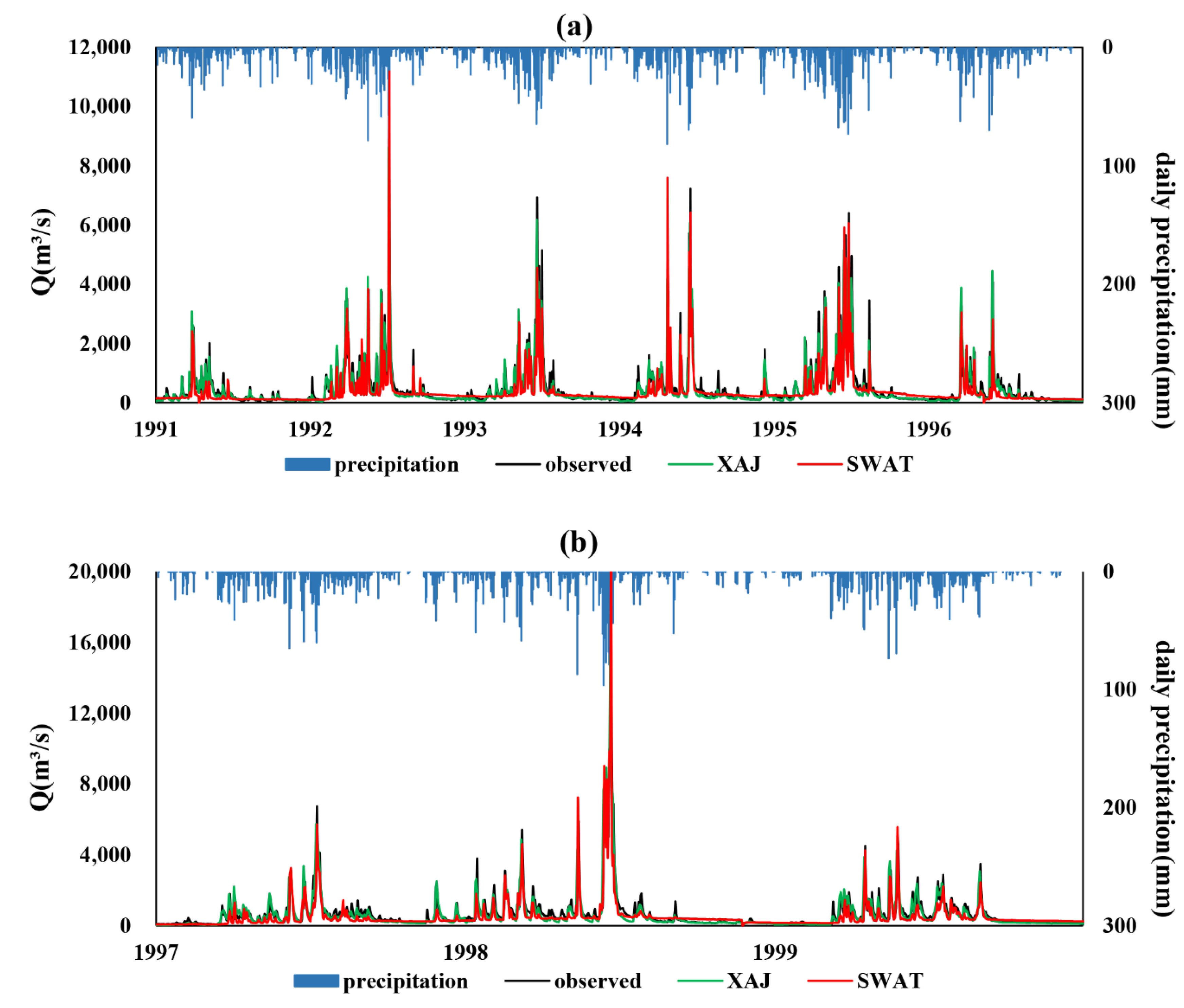
The performance of the SWAT model was nearly positively correlated with precipitation. The annual precipitation for 1992, 1995, 1997 and 1998 were all above 2000 mm. Simulation of daily discharge of these years was better in terms of R² and NSE. The annual precipitation for 1991 and 1996 was smaller and the simulation of these two years was much worse. Figure 3a, b show the time series of observed data and simulation results of the XAJ model and the SWAT model during the calibration and validation periods. During both the calibration and validation periods, the SWAT model simulated better than the XAJ model during flood season. This is very important because about 60% of the precipitation fell in flood season. Generally, the daily simulation results obtained from the XAJ and SWAT models demonstrated decent applicability and could consequently represent a preliminary basis for further event-based floods simulation.

3.3. Analysis of Model Performance in Flood Simulation

3.3.1. Simulation Results

Calibration and validation of the sub-daily SWAT model in flood simulation were conducted using SWAT-CUP and a few modifications were made to it to accommodate the hourly time-scale input. The results of calibration and validation for XAJ and the sub-daily SWAT model are listed in

Table 5. Parameter sensitivities for SWAT model in daily and flood simulation.

Period	Flood Code	Runoff (mm)			Peak(m3/s)			RRE (%)		RPE (%)		PTE(h)
		Observed	XAJ	SWAT	Observed	XAJ	SWAT	XAJ	SWAT	XAJ	SWAT	XAJ	SWAT
	910326	78.9	76.2	69.8	3180	3530	2950	3.42	11.53	−11.01	7.23	42	39
	910426	49.7	46.3	20.8	1730	1757	883	6.84	58.15	−1.58	48.96	148	−3
	910617	12.7	12.0	12.9	958	1132	1080	5.51	−1.57	−18.19	−12.73	−22	−24
	920321	130.7	85.9	116.1	4330	4351	3580	34.28	11.17	−0.48	17.32	−6	−5
	920501	37.0	35.4	38.0	2210	2553	2620	4.32	−2.70	−15.50	−18.55	134	−13
	920514	81.1	69.5	74.3	6920	7933	5680	14.30	8.38	−14.64	17.92	−5	−4
	920616	80.3	77.1	68.3	6300	6811	5440	3.99	14.94	−8.10	13.65	−4	−1
	920704	182.3	162.9	203.5	10,700	12,157	15,700	10.64	−11.63	−13.62	−46.73	−8	−9
	920831	24.3	24.6	19.5	2080	2444	1810	−1.23	19.75	−17.50	12.98	7	−6
	930502	76.5	44.7	64.8	3730	3629	3140	41.57	15.29	2.71	15.82	−8	−9
Calibration	930523	96.1	94.3	81.0	2740	3254	2250	1.87	15.71	−18.77	17.88	−23	−160
	930615	198.3	190.4	145.6	9710	9509	8900	3.98	26.58	2.07	8.34	−7	−11
	940425	95.3	85.5	118.2	7250	7668	10,900	10.28	−24.03	−5.77	−50.34	−4	−6
	940521	62.4	62.8	54.1	4000	4727	2540	−0.64	13.30	−18.16	36.50	−4	8
	940614	131.1	89.3	114.6	9240	11,787	9560	31.88	12.59	−27.57	−3.46	−6	−6
	950424	168.2	147.6	138	4560	5248	3660	12.25	17.95	−15.09	19.74	−5	71
	950603	96.5	91.2	87.2	6650	6989	5530	5.49	9.64	−5.09	16.84	93	−2
	950614	187.9	146.3	165	7650	9934	7570	22.14	12.19	−29.86	1.05	50	−7
	950625	137.3	133.1	120.3	11,100	12,795	12,500	3.06	12.38	−15.27	−12.61	−7	−7
	950813	40.7	47.3	26.7	4310	4912	2330	−16.22	34.40	−13.98	45.94	−2	4
	960317	82.0	85.1	86.1	4140	4281	3680	−3.78	−5.00	−3.40	11.11	−3	−4
	960530	81.2	81.8	50.1	4620	4910	3460	−0.74	38.30	−6.27	25.11	32	30
	average	96.8	85.9	85.2	5369	6014	5262	8.78	13.06	−11.59	7.82	18	−6
	970605	63.8	68.2	66.0	5760	5247	5630	−6.90	−3.45	8.91	2.26	−7	−3
	970620	59.5	45.1	64.0	3820	4463	3120	24.20	−7.56	−16.83	18.32	−3	−6
	970702	134.5	130.9	108.9	7770	9081	7070	2.68	19.03	−16.87	9.01	−8	−6
	970808	35.9	32.6	35.4	1490	1734	2090	9.19	1.39	−16.34	−40.27	−7	−9
	980215	34.9	36.5	37.5	3790	3651	3860	−4.58	−7.45	3.68	−1.85	−7	−9
	980301	137.6	133.8	115.1	5810	6943	5430	2.76	16.35	−19.49	6.54	−25	−9
	980509	99.3	94.1	91.5	10,400	12,358	11400	5.24	7.85	−18.83	−9.62	−7	−4
Validation	980608	253.2	220	237.7	12,100	14,675	13400	13.11	6.12	−21.28	−10.74	62	59
	980619	419.1	407	368.7	21,600	23,217	29600	2.89	12.03	−7.49	−37.04	−8	−10
	990415	61.9	71.3	65.7	6360	6726	6570	−15.19	−6.14	−5.75	−3.30	−3	−3
	990515	63.3	67.1	58.0	3950	4240	3300	-6.00	8.37	−7.34	16.46	−13	−16
	990523	94.9	95.8	85.6	7910	9018	7780	-0.95	9.80	−14.01	1.64	−10	−7
	990715	80.9	62.5	64.7	4420	5239	3070	22.74	20.02	−18.54	30.54	−6	−8
	990825	83.9	91.3	68.6	3990	4600	2880	-8.82	18.24	−15.28	27.82	1	−1
	average	115.9	111.2	104.8	7084	7942	7514	2.88	6.76	−11.82	0.70	−3	−2

. During the calibration period, the sub-daily SWAT model performed better than the XAJ model with R² ranging from 0.5 to 0.89 and NSE ranging from 0.33 to 0.85, compared with 0.07 to 0.92 and 0.2 to 0.92 of R² and NSE for the XAJ model, respectively. During the validation period, both of these models improved. The average R², NSE and PBIAS for the SWAT model was 0.73, 0.56 and −6.76, respectively, and the average R², NSE and PBIAS for the XAJ model was 0.65, 0.50 and −2.88, respectively. Generally, the SWAT model did better than the XAJ model according to R² and NSE. The results of NSE values were better than a previous study [18], as the model had been calibrated and validated over flood periods only.

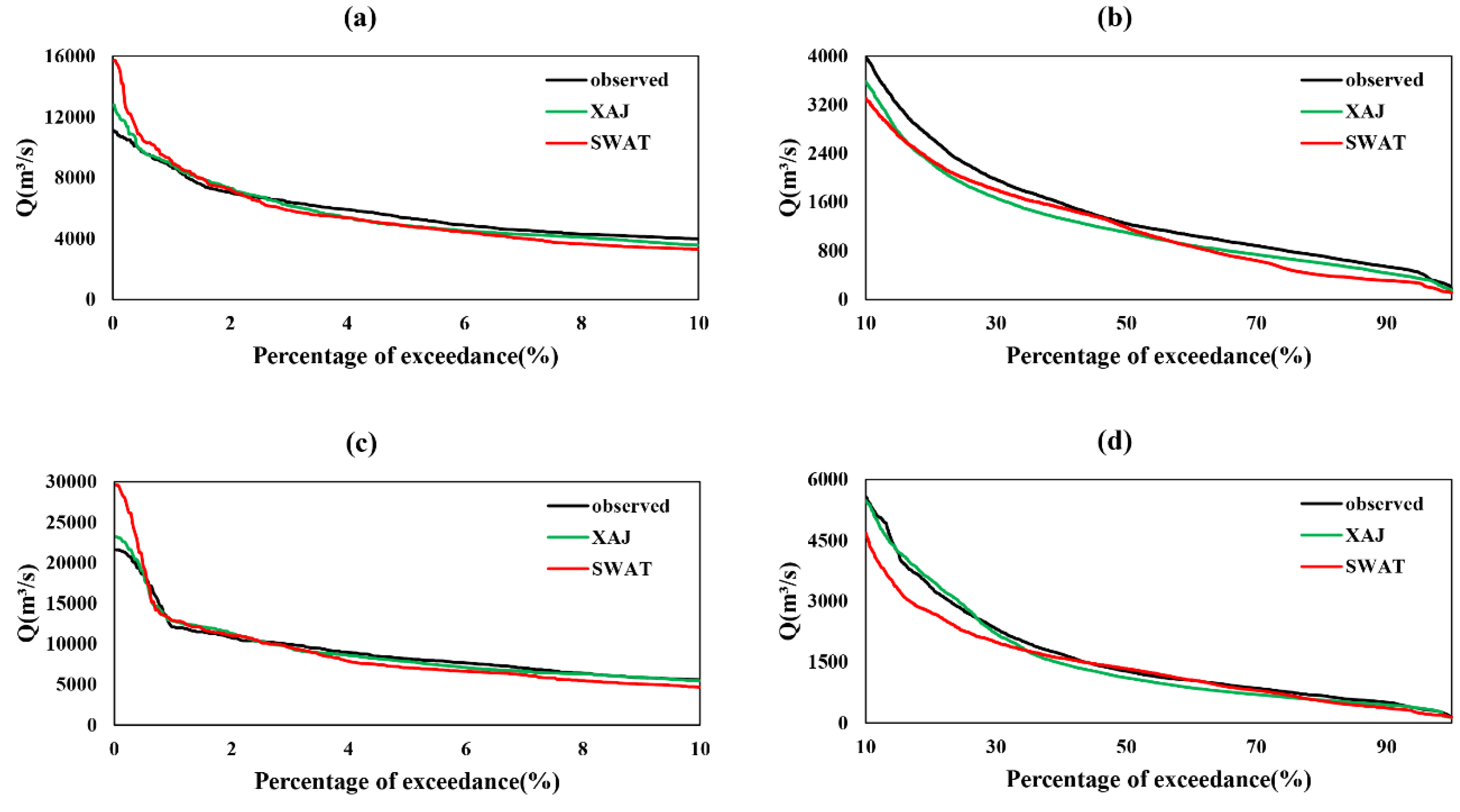
We also plotted flow duration curves (FDCs) in Figure 4 to evaluate the agreement between observations and simulations. Both the XAJ and SWAT models overestimated extreme high flows (<1% exceedance) during calibration and validation periods, and it was further obvious in the SWAT model. While the SWAT model could capture high flows (~2% exceedance) perfectly. During the calibration period, the SWAT model predicted better in terms of medium flows (~50% exceedance) but had a poor performance in terms of low flows. During the validation period, it was the opposite. The XAJ model performed satisfactorily in estimating medium flows while the SWAT model had better agreement in low flows. Both of the two models overestimated high flows and underestimated low flows as a whole. The models responded differently to extremely high and extremely low flows. Therefore, the responses of the models to different conditions [39,40,41] need further study.

3.3.2. Performance of SWAT and XAJ Model in Event-Based Floods

Table 5 summarizes the statistical performance measures for runoff, peak flow and occurrence time of peak flow. During the calibration period, the average RRE and RPE of the XAJ model were −8.78% and 11.59%, respectively, while the two values of the SWAT model were −13.06% and −7.82%, respectively. The SWAT model simulated better in terms of RPE. During the validation period, it showed the same conclusion. The distributed model consistently performed better than the lumped model in simulating peak flow [42]. However, we need to consider the simulation of each single event-based flood to evaluate the event-based flood simulation capability of the SWAT model. Depending on the standard, the XAJ model simulated better than SWAT. There were four floods unqualified during the calibration period and three floods unqualified during the validation period. Meanwhile, there were six floods and four floods unqualified during the calibration and validation periods of the SWAT model, respectively. Both the XAJ and SWAT model reproduced the event-based floods fairly well. The error of occurrence time of peak flow (PTE) for each flood was also calculated. The SWAT model performed better than the XAJ model. The average values of PTE of the SWAT model during calibration and validation period were −6 h and −2 h, respectively, while the average values of the XAJ model were 18 h and −3 h, respectively. Both the XAJ and SWAT models could simulate the occurrence time of peak flow well during the validation period. However, the XAJ model predicted unsatisfactorily during the calibration period with the average PTE of 18 h, which indicated that the peak flow simulated by the XAJ model occurred later than the measured peak flow overall. The SWAT model can capture the occurrence time of peak flow perfectly and this is crucial for flood forecasting.

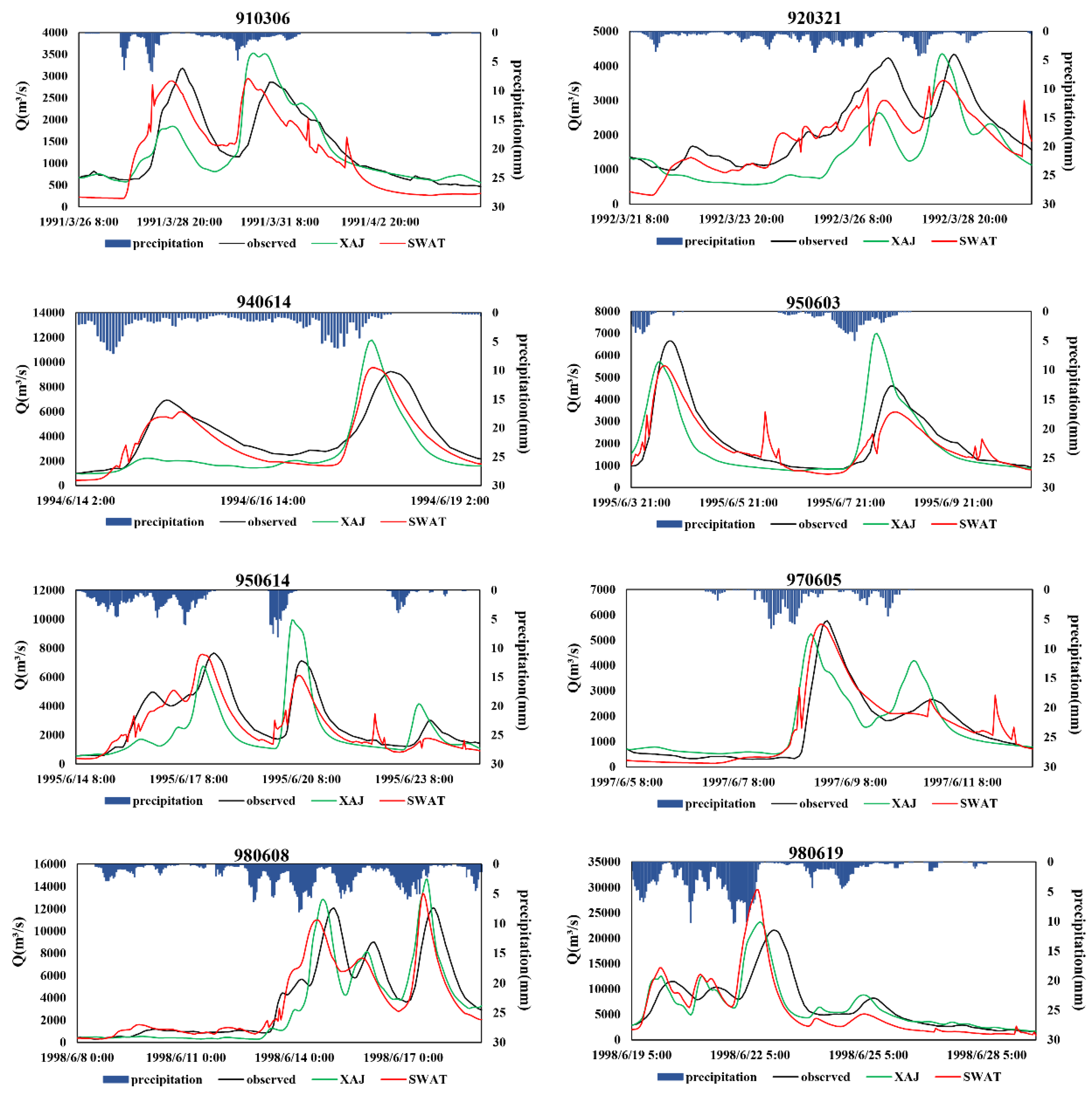
Figure 5 compared observed and simulated discharges by XAJ and SWAT models for eight event-based floods. The SWAT model had a poor performance in the beginning of most floods and it was particularly evident in the first flood of the year (Flood 910306, 920321 and 970605). It tended to underestimate the low flows. It is implied that antecedent conditions are very important for the model simulation [16]. In the XAJ model, initial hydrological information of event-based floods, such as soil moisture content, was captured through daily simulation. Even though we used the same method in the SWAT model, the results were still limited by precipitation data. As mentioned above, hourly precipitation data were only available during floods and the data during non-flood periods were obtained from daily precipitation. This may bring some error to the calculation of initial hydrological information of floods, especially the first flood of the year. The rain gauges resolution and accuracy of measurements were very important and may affect the model outputs [43]. During extreme events, precipitation measurements may not be accurate [44]. Therefore, in extreme flood (Flood 980619), the SWAT model vastly overestimated the peak flow. The same conclusions could also be found in the FDCs. Recession flows were also badly simulated. This might be ascribed to the calculation of base flow. Base flow was calculated at daily time-scale and had an equal distribution of the daily estimates to each time step. Though the SWAT model had a poor performance in low flows, it had an improvement in simulating high and medium flows [15,18]. As mentioned above, the SWAT model performed better in terms of RPE, and this is particularly evident in the picture (Flood 940614, 950614, 970605 and 980608). It is worth noting that all of these floods had multiple peak flows. This showed that the SWAT model was capable of capturing multiple flood peaks accurately.

3.4. Effect of Spatial Scale on SWAT Model

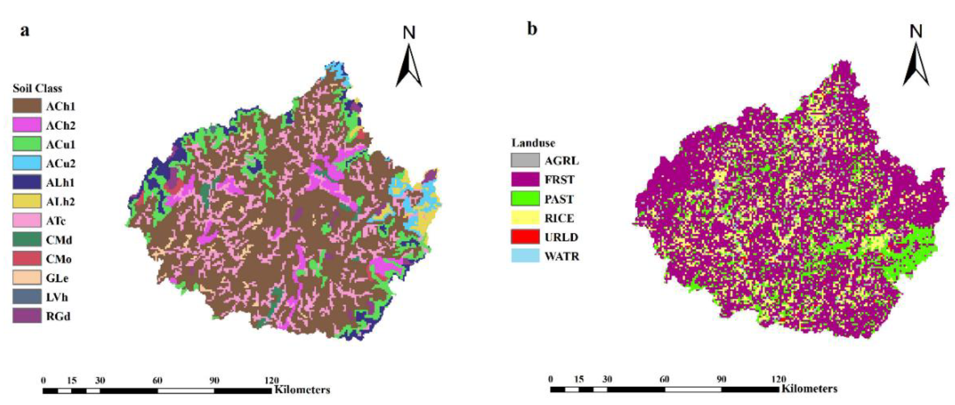
Due to the spatial heterogeneity of hydrological conditions of a river basin, such as topography, land use and soil type, hydrological phenomena also change accordingly. Research on the spatial scale is very important for the application of hydrological models. It is of great practical significance to utilize the hydrological data of a larger basin to deduce the hydrological characteristics of a smaller watershed.

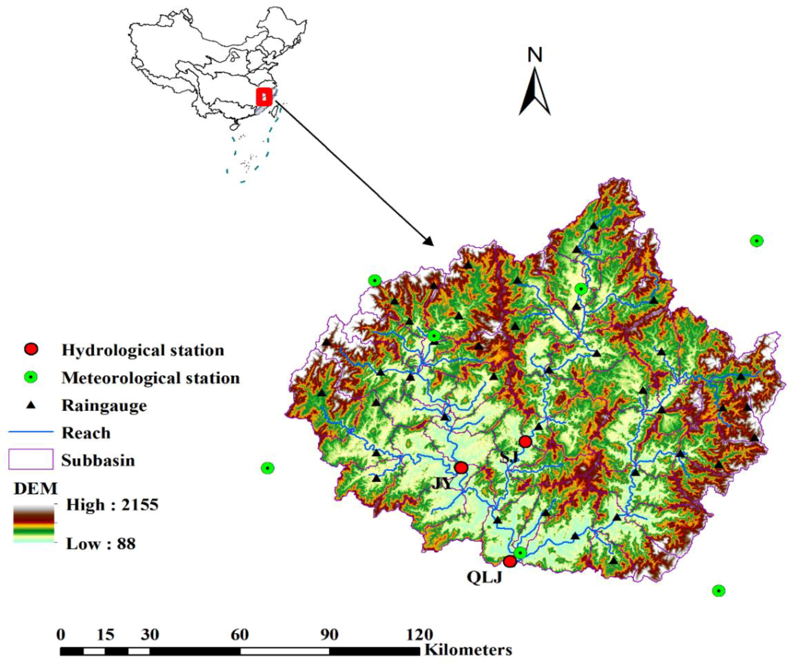
To evaluate the effect of spatial scale on the SWAT model, the team took JY and SJ station as an example. Their locations are marked in Figure 1 and the basic information of these three stations is presented in

Table 6. Basic information of QLJ, JY and SJ stations.

Category	Data Type	QLJ	JY	SJ
Topography	Catchment Area (km2)	14800	4846	3390
	Slop (%)	28.4	28.6	27.6
	Elevation (m)	423	397	460
Land use	Forest (%)	65.17	70.53	64.65
	Pasture (%)	14.45	10.04	10.39
	Agriculture (%)	19.26	18.7	23.97
Soil	Haplic Acrisols (%)	60.3	55.67	67.3
	Cumulic Anthrosols (%)	15.6	16.7	15.5
	Humic Acrisols (%)	12.2	12.99	9.8

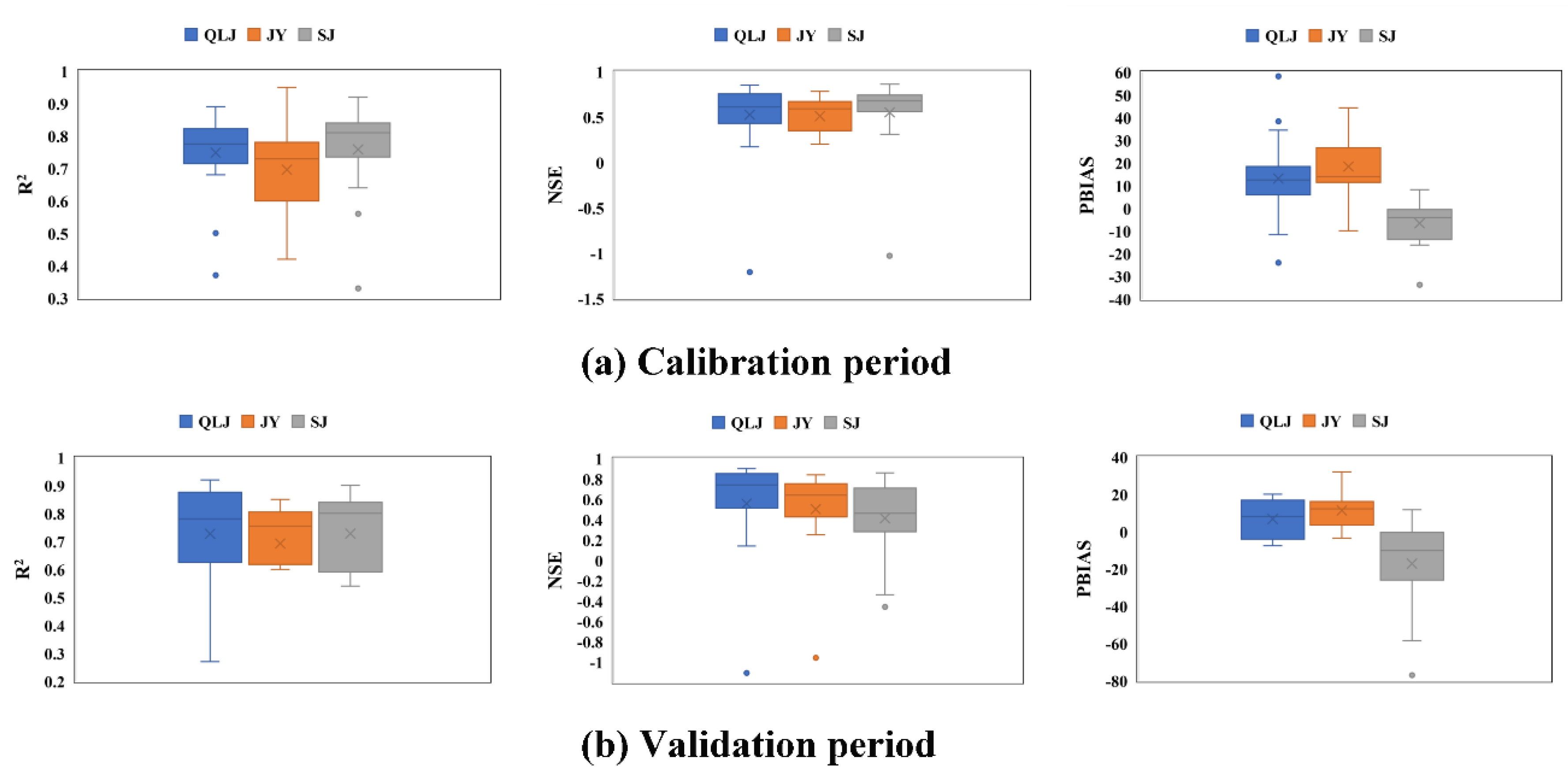
. The catchment areas of JY and SJ station were much smaller than the area of QLJ station. There were also some differences in their land use and soil types. We simulated floods in JY and SJ stations using the parameters calibrated by QLJ station and calculated R², NSE and PBIAS for each flood. Figure 6 shows the boxplots of R², NSE and PBIAS for these three stations. During the calibration period, R² and NSE of these stations did not change much. However, they had a different reaction according to PBIAS. The PBIAS values of QLJ and JY station were 13.06 and 18.42, respectively, while the PBIAS value of SJ station was −6.28. It is implied that the SWAT model underestimated flow regimes in QLJ and JY stations but overestimated flow regimes in SJ station. On the whole, SJ station behaved the best during the calibration period. During the validation period, the SWAT model performed better in QLJ station. JY station showed good consistency with QLJ station while SJ station had the worst performance.

The qualification ratios of these three stations were also summarized according to the standard mentioned above. In QLJ station, there were 25 floods qualified among 36 floods, the qualified ratio was 69.4%. While there were 20 floods qualified among 33 floods in JY station and 20 floods qualified among 30 floods in SJ station. The qualified ratio was 60.6% and 66.7%, respectively. Among 25 floods qualified in QLJ station, 16 floods were likewise qualified in JY station and 14 floods were qualified in SJ station. About half of the floods qualified in QLJ station were qualified in JY and SJ station simultaneously. The results showed that the SWAT model had a good applicability at different spatial scales.

4. Conclusions

The SWAT model has been extensively used for long-term simulations with daily, monthly or yearly time-scales. This paper developed the sub-daily SWAT model for Qilijie basin. We evaluated the sub-daily SWAT model in flood simulation and compared it with the XAJ model.

Both the XAJ and SWAT models behaved satisfactorily in the simulation of event-based floods and had a similar qualified ratio. The XAJ model performed better than the sub-daily SWAT model in terms of RRE, but sub-daily SWAT had a better performance in reproducing peak flow and was good at capturing the occurrence time of peak flow. The sub-daily SWAT model had an improvement in simulating high and medium flows and had showed its capacity of simulating floods with multiple peaks accurately. Hence, the SWAT model has great potential for flood simulation.

The effect of spatial scale on the SWAT model was also evaluated in this research. The results showed that the SWAT model had a good applicability at different spatial scales and could deduce the hydrological characteristics of a smaller watershed using parameters from a larger basin. This is a valuable reference to research the effect of spatial scale on hydrological models.

However, the performance of the SWAT model in flood simulation was affected by precipitation data. Hourly time-scale precipitation data were only available during flood seasons in China and we estimated hourly precipitation during non-flood periods by assuming a uniform distribution in daily precipitation. Hence, the SWAT model simulated badly in the beginning of floods and it would perform better with accurate precipitation input. The SWAT model also performed poorly in estimating low flows and this might be attributed to the daily calculation of base flow. The feasibility of using the sub-daily SWAT model for flood simulation in large regulated regions remains to be further studied.

References

1. Crawford, N.H.; Linsley, R.K. Digital Simulation in Hydrology: Stanford Watershed Model IV; Department of Civil Engineering, Stanford University: Stanford, CA, USA, 1966. [Google Scholar]
2. Zhao, R.J.; Zhang, Y.L.; Fang, L.R.; Liu, X.R.; Zhang, Q.S. The Xinanjiang Model. 1980. Available online: http://hydrologie.org/redbooks/a129/iahs_129_0351.pdf (accessed on 24 March 2018).
3. Li, Z.J.; Bao, H.J.; Xue, C.S.; Hu, Y.Z.; Fang, H. Real-time flood forecasting of Huai River with flood diversion and retarding areas. Water Sci. Eng. 2008, 1, 10–24. [Google Scholar]
4. Liu, J.T.; Chen, X.; Zhang, J.B.; Flury, M. Coupling the Xinanjiang model to a kinematic flow model based on digital drainage networks for flood forecasting. Hydrol. Process. 2009, 23, 1337–1348. [Google Scholar] [CrossRef]
5. Rossman, L.A. Storm Water Management Model User’s Manual Version 5.0; National Risk Management Research Laboratory, Office of Research and Development, U.S. Environmental Protection Agency: Cincinnati, OH, USA, 2004.
6. Bicknell, B.; Imhoff, J.; Kittle, J.; Donigian, A.; Johanson, R. Hydrological Simulation Program—FORTRAN: User’s Manual for Version 11; United States Environmental Protection Agency, National Exposure Research Laboratory: Athens, GA, USA, 1997; p. 755.
7. Abbott, M.B.; Bathurst, J.C.; Cunge, J.A.; O’Connell, P.E.; Rasmussen, J. An introduction to the European Hydrological System—Systeme Hydrologique Europeen, “SHE”, 1: History and philosophy of a physically-based, distributed modelling system. J. Hydrol. 1986, 87, 61–77. [Google Scholar] [CrossRef]
8. Young, R.A.; Onstad, C.A.; Bosch, D.D.; Anderson, W.P. AGNPS: A Non-Point-Source Pollution Model for Evaluating Agricultural Watersheds. J. Soil Water Conserv. 1989, 44, 168–173. [Google Scholar]
9. Beasley, D.; Hyggins, L. ANSWERS: User’s Manual; U.S. Environmental Protection Agency: Chicago, IL, USA, 1995.
10. Arnold, J.G.; Srinivasan, R.; Muttiah, R.S.; Williams, J.R. Large area hydrologic modeling and assessment part I: Model development. J. Am. Water Resour. Assoc. 1998, 34, 73–89. [Google Scholar] [CrossRef]
11. Roux, H.; Labat, D.; Garambois, P.A.; Maubourguet, M.M.; Chorda, J.; Dartus, D. A physically-based parsimonious hydrological model for flash floods in Mediterranean catchments. Nat. Hazards Earth Syst. Sci. 2011, 11, 2567–2582. [Google Scholar] [CrossRef] [Green Version]
12. Ouyang, W.; Hao, F.H.; Song, K.Y.; Zhang, X. Cascade Dam-Induced Hydrological Disturbance and Environmental Impact in the Upper Stream of the Yellow River. Water Resour. Manag. 2011, 25, 913–927. [Google Scholar] [CrossRef]
13. Zhang, Y.Y.; Xia, J.; Liang, T.; Shao, Q.X. Impact of Water Projects on River Flow Regimes and Water Quality in Huai River Basin. Water Resour. Manag. 2010, 24, 889–908. [Google Scholar] [CrossRef]
14. Shi, P.; Chen, C.; Srinivasan, R.; Zhang, X.S.; Cai, T.; Fang, X.Q.; Qu, S.M.; Chen, X.; Li, Q.F. Evaluating the SWAT Model for Hydrological Modeling in the Xixian Watershed and a Comparison with the XAJ Model. Water Resour. Manag. 2011, 25, 2595–2612. [Google Scholar] [CrossRef]
15. Jeong, J.; Kannan, N.; Arnold, J.; Glick, R.; Gosselink, L.; Srinivasan, R. Development and integration of sub-hourly rainfall—Runoff modeling capability within a watershed model. Water Resour. Manag. 2010, 24, 4505–4527. [Google Scholar] [CrossRef]
16. Yu, D.; Xie, P.; Dong, X.H.; Hu, X.N.; Liu, J.; Li, Y.H.; Peng, T.; Ma, H.B.; Wang, K.; Xu, S.J. Improvement of the SWAT model for event-based flood forecasting on a sub-daily time scale. Hydro. Earth System Sci. 2017. [Google Scholar] [CrossRef]
17. Yang, X.Y.; Liu, Q.; He, Y.; Luo, X.Z.; Zhang, X.X. Comparison of daily and sub-daily SWAT models for daily streamflow simulation in the Upper Huai River Basin of China. Stoch. Env. Res. Risk A. 2016, 30, 959–972. [Google Scholar] [CrossRef] [Green Version]
18. Boithias, L.; Sauvage, S.; Lenica, A.; Roux, H.; Abbaspour, K.C.; Larnier, K.; Dartus, D.; Sánchez-Pérez, J.M. Simulating flash floods at hourly time-step using the SWAT model. Water 2017, 9, 929. [Google Scholar] [CrossRef]
19. Zhao, R.J. The Xinanjiang model applied in China. J. Hydrol. 1992, 135, 371–381. [Google Scholar]
20. Zhao, R.J. A non-linear system model for basin concentration. J. Hydrol. 1993, 142, 477–482. [Google Scholar]
21. Fontaine, T.A.; Cruickshank, T.S.; Arnold, J.G.; Hotchkiss, R.H. Development of a snowfall-snowmelt routine for mountainous terrain for the soil water assessment tool (SWAT). J. Hydrol. 2002, 262, 209–223. [Google Scholar] [CrossRef]
22. Bouraoui, F.; Benabdallah, S.; Jrad, A.; Bidoglio, G. Application of the SWAT model on the Medjerda river basin (Tunisia). Phys. Chem. Earth 2005, 30, 497–507. [Google Scholar] [CrossRef]
23. Zhang, A.J.; Zhang, C.; Fu, G.B.; Wang, B.D.; Bao, Z.X.; Zheng, H.X. Assessments of impacts of climate change and human activities on runoff with SWAT for the Huifa River Basin, Northeast China. Water Resour. Manag. 2012, 26, 2199–2217. [Google Scholar] [CrossRef]
24. Shi, P.; Ma, X.; Hou, Y.; Li, Q.; Zhang, Z.; Qu, S.; Chen, C.; Cai, T.; Fang, X. Effects of land-use and climate change on hydrological processes in the upstream of Huai River, China. Water Resour. Manag. 2013, 27, 1263–1278. [Google Scholar] [CrossRef]
25. Monteith, J.L. Evaporation and environment. Symp. Soc. Exp. Biol. 1965, 19, 205–234. [Google Scholar] [PubMed]
26. Neitsch, S.L.; Arnold, J.G.; Kiniry, J.R.; Williams, J.R. Soil and Water Assessment Tool Theoretical Documentation, version 2009; Texas Water Resources Institute Technical Report No. 406; Texas A&M University System: College Station, TX, USA, 2011. [Google Scholar]
27. Arnold, J.G.; Kiniry, J.R.; Srinivasan, R.; Williams, J.R.; Haney, E.B.; Neitsch, S.L. Soil & Water Assessment Tool Input/Output Documentation, Version 201; Texas Water Resources Institute Technical Report No. 439; Texas A & M University: Temple, TX, USA.
28. Arnold, J.G.; Allen, P.M.; Bernhardt, G. A comprehensive surface-groundwater flow model. J. Hydrol. 1993, 142, 47–69. [Google Scholar] [CrossRef]
29. Williams, J.R. Flood routing with variable travel time or variable storage coefficients. Trans. ASABE 1969, 12, 100–103. [Google Scholar] [CrossRef]
30. Overton, D.E. Muskingum flood routing of upland streamflow. J. Hydrol. 1966, 4, 185–200. [Google Scholar] [CrossRef]
31. Luo, Y.X.; Su, B.L.; Yuan, J.Y.; Li, H.; Zhang, Q. GIS techniques for watershed delineation of SWAT model in plain polders. Procedia Environ. Sci. 2011, 10, 2050–2057. [Google Scholar] [CrossRef]
32. Abbaspour, K.C.; Yang, J.; Maximov, I.; Siber, R.; Bogner, K.; Mieleitner, J.; Zobrist, J.; Srinivasan, R. Modelling hydrology and water quality in the pre-alpine/alpine Thur watershed using SWAT. J. Hydrol. 2007, 333, 413–430. [Google Scholar] [CrossRef]
33. Abbaspour, K.C.; Johnson, C.A.; van Genuchten, M.T. Estimating Uncertain flow and transport parameters using a sequential uncertainty fitting procedure. Vadose Zone J. 2004, 3, 1340–1352. [Google Scholar] [CrossRef]
34. Abbaspour, K.C.; Rouholahnejad, E.; Vaghefi, S.; Srinivasan, R.; Yang, H.; Kløve, B. A continental-scale hydrology and water quality model for Europe: Calibration and uncertainty of a high-resolution large-scale SWAT model. J. Hydrol. 2015, 524, 733–752. [Google Scholar] [CrossRef]
35. Nash, J.E.; Sutcliffe, J.V. River flow forecasting through conceptual models: Part I—A discussion of principles. J. Hydrol. 1970, 10, 282–290. [Google Scholar] [CrossRef]
36. Gupta, H.V.; Sorooshian, S.; Yapo, P.O. Status of automatic calibration for hydrologic models: comparison with multilevel expert calibration. J. Hydrol. Eng. 1999, 4, 135–143. [Google Scholar] [CrossRef]
37. Moriasi, D.N.; Arnold, J.G.; Van Liew, M.W.; Bingner, R.L.; Harmel, R.D.; Veith, T.L. Model evaluation guidelines for systematic quantification of accuracy in watershed simulations. Trans. ASABE 2007, 50, 885–900. [Google Scholar] [CrossRef]
38. Kouchi, D.H.; Esmaili, K.; Faridhosseini, A.; Sanaeinejad, S.H.; Khalili, D.; Abbaspour, K.C. Sensitivity of calibrated parameters and water resource estimates on different objective functions and optimization algorithms. Water 2017, 9, 384. [Google Scholar] [CrossRef]
39. Wang, Y.L.; Yang, X.L. Sensitivity analysis of the surface runoff coefficient of hipims in simulating flood processes in a large basin. Water 2018, 10, 253. [Google Scholar] [CrossRef]
40. Kuriqi, A.; Ardiçlioglu, M.; Muceku, Y. Investigation of seepage effect on river dike’s stability under steady state and transient conditions. Pollack Periodica 2016, 11, 87–104. [Google Scholar] [CrossRef]
41. Kuriqi, A.; Ardiçlioǧlu, M. Investigation of hydraulic regime at middle part of the Loire River in context of floods and low flow events. Pollack Periodica 2018, 13, 145–156. [Google Scholar] [CrossRef]
42. Carpenter, T.M.; Georgakakos, K.P. Intercomparison of lumped versus distributed hydrologic model ensemble simulations on operational forecast scales. J. Hydrol. 2006, 329, 174–185. [Google Scholar] [CrossRef]
43. Grusson, Y.; Anctil, F.; Sauvage, S.; Sánchez-Pérez, J.M. Testing the SWAT model with gridded weather data of different spatial resolutions. Water 2017, 9, 54. [Google Scholar] [CrossRef]
44. Omranian, E.; Sharif, H.O.; Tavakoly, A.A. How well can global precipitation measurement (GPM) capture hurricanes? case study: hurricane Harvey. Remote Sens. 2018, 10, 1150. [Google Scholar] [CrossRef]
Figure 1. Location of Qilijie Basin and its stations.
Water 10 01263 g001
Figure 2. Soil map (a)and land use (b) in Qilijie Basin.
Water 10 01263 g002
Figure 3. (a) Comparisons between the observed and simulated daily discharge for the calibration period and (b) comparisons between the observed and simulated daily discharge for the validation period. For better readability, the maximal of Y axes in (b) was limited to 20,000 m3/s. So, some of the maximum discharge, i.e., 20,290 m3/s, were not shown in the figure.
Water 10 01263 g003
Figure 4. Observed and simulated flow duration curves: (a) flow duration curves (FDCs) for high flows during calibration period; (b) flow duration curves (FDCs) for medium and low flows during calibration period; (c) flow duration curves (FDCs) for high flows during validation period; (d) flow duration curves (FDCs) for medium and low flows during validation period.
Water 10 01263 g004
Figure 5. Comparison of simulation of floods conducted using XAJ and SWAT models.
Water 10 01263 g005
Figure 6. Boxplots of R2, NSE and PBIAS. In each boxplot, the whisker ranges from the minimum to maximum, while the box ranges from the first quartile to the third quartile. The symbol cross represents the mean value and the symbol circle dot represents the outlier.
Water 10 01263 g006