Assessment of Aquatic Weed in Irrigation Channels Using UAV and Satellite Imagery


Centre for Regional and Rural Futures, Deakin University, Geelong 3220, Australia
*
Author to whom correspondence should be addressed.
Water 2018, 10(11), 1497; https://doi.org/10.3390/w10111497
Submission received: 8 October 2018
/
Revised: 17 October 2018
/
Accepted: 18 October 2018
/
Published: 23 October 2018
(This article belongs to the Special Issue Data-Driven Methods for Agricultural Water Management)
Abstract
:Irrigated agriculture requires high reliability from water delivery networks and high flows to satisfy demand at seasonal peak times. Aquatic vegetation in irrigation channels are a major impediment to this, constraining flow rates. This work investigates the use of remote sensing from unmanned aerial vehicles (UAVs) and satellite platforms to monitor and classify vegetation, with a view to using this data to implement targeted weed control strategies and assessing the effectiveness of these control strategies. The images are processed in Google Earth Engine (GEE), including co-registration, atmospheric correction, band statistic calculation, clustering and classification. A combination of unsupervised and supervised classification methods is used to allow semi-automatic training of a new classifier for each new image, improving robustness and efficiency. The accuracy of classification algorithms with various band combinations and spatial resolutions is investigated. With three classes (water, land and weed), good accuracy (typical validation kappa >0.9) was achieved with classification and regression tree (CART) classifier; red, green, blue and near-infrared (RGBN) bands; and resolutions better than 1 m. A demonstration of using a time-series of UAV images over a number of irrigation channel stretches to monitor weed areas after application of mechanical and chemical control is given. The classification method is also applied to high-resolution satellite images, demonstrating scalability of developed techniques to detect weed areas across very large irrigation networks.
1. Introduction
Much of the food and fibre needs of the world are met with irrigated agriculture. A large proportion of the farms devoted to this are supplied by networks of channels, which are seeing increasing levels of automation [1]. Excessive vegetation in these typically earthen channels impacts timely and efficient delivery of water to farms because of its effect of reducing flow rates [2]. Relationships between channel geometry, aquatic weed growth and Manning’s resistance coefficient n for rivers were explored in [3]. Monitoring and controlling weeds in irrigation channels is a costly exercise, and there is therefore demand to improve the effectiveness of monitoring and methods of assessing new control strategies.
Irrigation channel networks often cover significant areas, with many kilometers of channels. For example, the Murrumbidgee Irrigation network covers a total of 670,000 ha, and delivered water to 117,900 ha of irrigated land in 2017. It includes 3500 km of supply channels and 1600 km of drainage channels [4]. The widths of these channels are typically less than 10 m, the depths less than 1.5 m, and the vast majority are earthen channels. These characteristics are similar to most irrigation areas in the world. Considering the vast distances involved, regular manual surveying channels for weeds is impractical.
Many works have considered alternatives of manual monitoring of aquatic vegetation, including echo sounding and remote sensing (optical and radar). Most of these studies focused on lakes and rivers rather than irrigation channels.
Echo sounding for vegetation detection in an estuary was investigated in [5]. Sonar detection of vegetation works by sensing reflections, probably caused by the presence of gas in plants, which causes an acoustic impedance discontinuity with the surrounding water. Unvegetated bottom returns the strongest signal, while vegetation returns a weaker echo (but still stronger than ambient water noise). They classify each ping return into unclassified, noise, out of water, too deep, bare bottom and plant. They performed physical sampling (over a quadrat), and visual analysis using video (clear water) to compare against sonar estimates of vegetation coverage. They found reasonable relationships, but suggested optical techniques are better for shallow water or for vegetation appearing on the surface. A comparison of spatial environmental models, echo sounding and remote sensing to predict vegetation distribution and biomass in a lake [6] found remote sensing was the least accurate in this environment due to water turbidity. This raises a difficulty in earthen irrigation channels, as the water is often turbid. Despite the advantages of echo sounding for vegetation mapping, it would be impractical to cover irrigation channel networks using this technique due to time and labour costs.
Stationary optical sensors may be useful to assess weed growth in fixed locations. Methods to eliminate reflections from the water surface using Red-Green-Blue (RGB) cameras were discussed in [7]. They trialled a number of solutions including a camera mounted in a tube breaking the water surface with the tube bottom 10 cm below the surface, an underwater camera on a floating frame, and dedicated underwater cameras facing up and down. While fixed sensors are attractive to monitor weed growth in irrigation channels due to the high temporal resolution, weeds often grow in small patches so it is possible that they would not be detected at sensor locations. A large number of sensors would be required to cover a network.
A theoretical background for remote sensing in aquatic areas was reviewed in [8]. They note that reflectance of electromagnetic signals differ depending on whether plants are submerged, floating or emergent, due to the significant and variable effect water has on different parts of the spectrum. Synthetic aperture radar uses the microwave part of the spectrum. Though it doesn’t penetrate water, it can be used to detect emergent vegetation, and the use of interferometry could be used to determine vegetation height. Use of Light Detecttion and Ranging (LiDAR) is challenging due to water absorption of the signal. The near infra-red portion of the spectrum is absorbed strongly by water, and thus optical reflectance is more useful for characterising submerged vegetation. They note the reasonable accuracy that has been achieved using even coarse resolution satellite imagery to predict vegetation cover and biomass. New vegetation indices were proposed and tested in [9] that aim to enhance separability between land and aquatic vegetation. An algorithm to correct the absorption of light by a water column above submerged aquatic vegetation (SAV) was developed in [10]. Optical images were able to determine the depth of SAV in clear water [11].
A manually-piloted radio-controlled aircraft with an RGB camera was used to detect and spray weeds including alligator weed and salvinia in an aquatic habitat in [12]. They used the Support Vector Machine (SVM) algorithm to classify images, with a weed expert providing the classification training set. An unmanned aerial vehicle (UAV) with red-green-blue (RGB) and near-infrared cameras was used to map the invasive water soldier weed in [13], using object-based image analysis and the random forest algorithm. They selected training samples throughout the area based on visual interpretation with four classes (water soldier emergent and submerged, native vegetation and other) and achieved a classification kappa of 61%. The relationship between remotely sensed aquatic vegetation areas and biomass in a lake was investigated in [14]. The best correlation was from the near infra-red band, with . These works indicate the promise of applying images captured by UAV and satellite to irrigation channel weed detection.
It is useful to be able to not only identify areas of aquatic vegetation in irrigation channels, but also to distinguish between species. This would allow analysis of a change of population of certain species, as well as targeted control for the dominant species in sections of channels. Species discrimination using field work is time consuming and only practical in small areas. The authors of [15] focus on discriminating wetland vegetation species and estimating their biophysical properties, using both multi- and hyper-spectral data. Challenges include the difficulty of identifying boundaries between aquatic vegetation (as they often overlap), and the reflectance characteristics of vegetation are often very similar and are combined with the reflectance characteristic of the surrounding water. In [16], lake and river sites were surveyed with with 5-cm resolution. They used visual inspection of the images to classify a large variety of weed species, and compared this with the accuracy of object-based image analysis and classification. Accuracy was better than 90% for water versus vegetation, and better than 50% for taxonomy. The possibility of plant species discrimination in estuaries using hyperspectral data was investigated in [17], considering variation in each species’ signature with space and time. Submerged plants can be discriminated only in visible wavelengths, as longer wavelengths (near infra-red) are absorbed by the water. The paper investigated three species, eelgrass Zostera capricorni, strapweed Posidonia australis, and paddleweed Halophila ovalis over two years. The green wavelengths were most significant in discriminating between species, followed by red. They give suggested wavelengths and bandwidths to optimally classify these species.
This work aims to apply remote sensing techniques to enable efficient detection of weed in irrigation channels. The challenges particular to this application include the narrow width of the channels (compared with previous works which focussed on larger bodies of water such as lakes and rivers). Irrigation networks are also sparse and spread over extensive areas, rather than concentrated in a tight area. In addition, irrigation channel water is often highly turbid. The study takes multispectral imagery from UAVs and satellites, processes them in Google Earth Engine (GEE) [18], using unsupervised and supervised classification algorithms to automatically map areas of weed infestation. This information is of great use to irrigation water delivery companies as they seek to optimise their networks to enable timely and high capacity delivery of water to farms.
2. Materials and Methods
2.1. Location
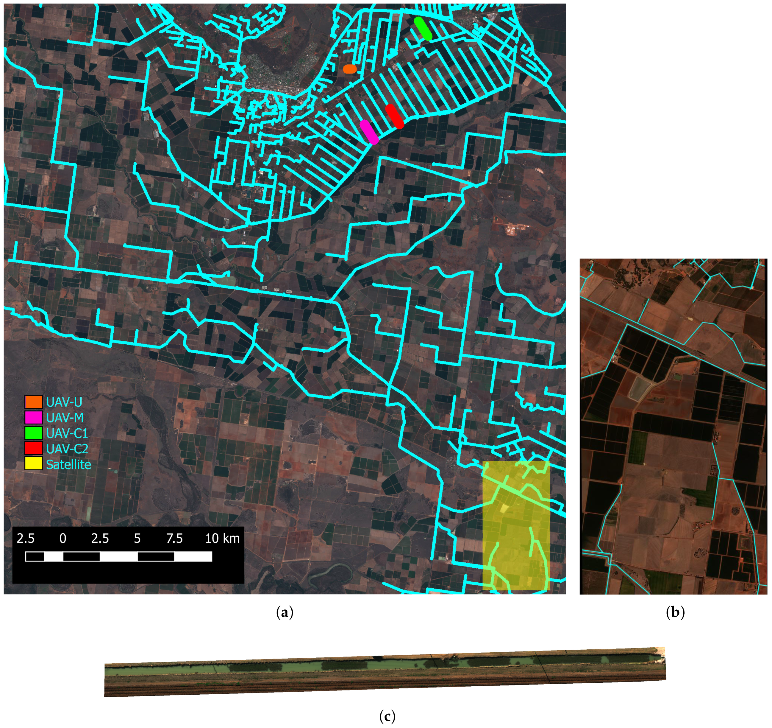
This study was based in the Murrumbidgee Irrigation Area (MIA), which includes the towns of Griffith, Whitton and Leeton in NSW, Australia. A wide variety of crops are grown in the area, with major summer crops including rice, cotton, citrus and grapes. The irrigation water is delivered by Murrumbidgee Irrigation, using a gravity-fed channel network from the Murrumbidgee River. The total irrigation area covers 670,000 ha, of which approximately 18% of the area was irrigated in 2017 [4]. A Sentinel-2 mosaic from January 2018 of a portion of the MIA is shown in Figure 1, centred at 342433.0 S, 1460153.9 E (WGS84). The figure contains annotations of the irrigation network supply channels, and of the areas mapped by UAV and satellite for this study.
2.2. Aquatic Vegetation
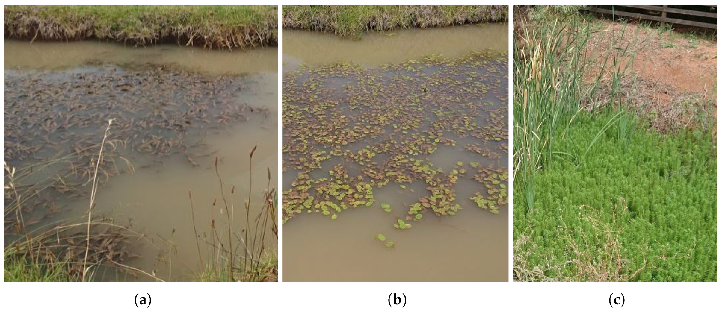
Four genera of aquatic vegetation grow in excess in MIA irrigation channels impeding flow and water delivery [19]. Three of the genera are native. One is cumbungi, Typha spp., an emergent flat leafed cylindrically stalked (2 cm diameter) reed that grows up to 4 m tall. Both T. domingensis and T. orientalis grow in the MIA region. They have clonal growth, with upright shots emerging each year from extensive underground rhizome beds. The other two genera of weedy vegetation are also attached to bottom of the channels, but their leaves float on the water surface. The ribbonweed Valliseneria spp. grows straplike leaves, 3 m long and 3 cm wide, from stolons in the sediment. In high nutrient waters, the green leaves appear brown as they are covered in algae. Both V. australis and V. nanna grow in the MIA, with V. nanna having a slightly narrower leave width. The third native genera of weedy plant in the MIA is pondweed Potamogeton spp. It has both submerged and floating leaves off stems up to 4 m long which grow out of rhizomes in the sediment. The floating leaves tend to be more robust, 10 cm long and 7 cm wide, than the translucent submerged leaves which are 20 cm long and 1 cm wide. Both P. tricarinatus and P. ochreatus grow in the MIA.
The introduced weedy vegetation is parrot’s feather Myriphyllum aquaticum, a native of South America. Stems of up to 2 m grow from rooted stolons and pale green, whorled and feathery leaves grow off the stems. Submerged leaves rot, leaving only the emergent leaves at the end of a long, bare submerged stem.
Potamogeton spp. grow rapidly in spring (September to November), followed by summer (December to February) growth of Valliseneria spp. Typha shoots can grow at any time of year, but the majority emerge in summer and autumn (March to May). Control of the biomass of the four genera in the irrigation channels is by different strategies and include both physical removal and chemical treatment. Photographs of the weed types is shown in Figure 2.
2.3. Image Capture
This study investigated the use of remotely-sensed multispectral imagery from both UAV and satellite platforms for detection of weed areas in irrigation channels.
2.3.1. UAV
UAV images were captured from a DJI (Shenzen, China) Inspire 1 v2. This is a quadcopter, weighing around 3 kg. A MicaSense (Seattle, WA, USA) RedEdge camera was attached to the UAV. Four of the five camera bands were used and are specified in Table 1. The flight paths were automated using the Drone Deploy iPad application. The images were captured from an altitude of 75 m with along-track overlap of 80% and at least two passes along the channel length. The ground pixel size was 5 cm. Before each flight, images of a calibration reflectance panel were taken. The images were radiometrically calibrated and orthomosaics were generated with the Pix4D software.
Images were captured over four channel stretches as part of a study of the effectiveness of different weed control strategies. To reduce the impact of shadowing, where possible, the images were taken within 2 h of solar noon. The treatments, channel dimensions and image capture dates are shown in Table 2. The untreated channel (U) had no weed control applied. The mechanical treatment channel (M) had excavator de-silting carried out on 23 July 2018. The two chemical treatment channels (C1 and C2) had Endothall herbicide applied on 11 July 2018.
Throughout the study period, each of the channels also had a WiField logger [20] continuously measuring water depth and temperature. Water depth was measured using a MaxBotix (Fort Mill, SC, USA) MB7389 ultrasonic sensor, and the water and air temperatures were measured using digital Maxim (Sunnyvale, CA, USA) DS18B20 temperature probes.
2.3.2. Satellite
In order to assess the effectiveness of the developed weed detection methods in classifying much larger areas of irrigation channels, two images from the World-View 3 satellite constellation were purchased. These were selected from the archive, on 7 January 2017 and 13 March 2018, with both captures occurring within 15 min of local noon. The common area between the images was used for analysis, covering 38.5 km. This covers part of the MIA around the town of Whitton, and the capture area is shown in Figure 1. The images had a pan-sharpened resolution of 30 cm, and eight multispectral bands. Four of the eight instrument bands were used, and are specified in Table 1.
2.4. Image Processing
Images from the UAV and satellites were uploaded to Google Earth Engine (GEE) as private assets. All subsequent image processing was performed in GEE, with some post analysis on data exported from GEE performed using Python. GEE allows quick and powerful cloud-based spatial data analysis, and includes algorithms for image co-registration, clustering and supervised classification [18].
2.4.1. World View-3 Satellite Image Pre-Processing
The World-View 3 satellite images are provided as 8-band digital number (DN) products. These images were pre-processed in GEE to obtain surface reflectance. First, they were converted to at-sensor radiance images using the data in [21]. Then, to obtain surface reflectance, the dark object subtraction (DOS) atmospheric correction method was applied [22].
2.4.2. UAV Image Co-Registration for Time-Series Analysis
The UAV orthomosaics were not co-registered. In order to define geometries marking areas common to all the images in the collection (for example geometries marking areas of land and channels), geo-location errors due to GPS inaccuracy need to be corrected. Thus, images were co-registered using the GEE registration algorithm. The images from each channel site were co-referenced to its corresponding 12 July image using the normalized difference vegetation index (NDVI) band.
2.4.3. Masking
A shapefile of the Murrumbidgee Irrigation supply channel network was obtained, and uploaded as a Google Fusion Table. This was then imported to GEE as a Feature Collection. To avoid problems with registration errors between the geometries in the supply channel features and the UAV and satellite images, the supply channel geometries were buffered by 10 m. These buffered geometries were then used to mask the images, so the resulting images only included the supply channels and a narrow region of land around the channels, with a total width of 20 m. This masking results in a reduced number of pixels to be processed. It also makes land area classification more accurate, as there is less variation in the reflectance characteristics of the land areas on either sides of the supply channels than that of the total land area of the unmasked images.
2.4.4. Vegetation Index Computation
Image bands were processed to give vegetation indexes, including the normalized difference vegetation index (NDVI), normalized difference water index (NDWI), normalized difference aquatic vegetation index (NDAVI), and visible atmospherically resistant index (VARI) among others [9,23,24]. The equations for the indices used are given in Table 3. Statistics for the each of the bands and indexes were computed over areas of interest.
2.4.5. Geometry Definition for Sampling
Polygon geometries were drawn on the images to identify areas of water, land, weed and channel (containing both water and weed). These areas are easily identifiable from red-green-blue images, so the polygons were drawn by visual inspection of the images. In each case, stratified sampling algorithms in GEE were used to randomly sample pixels within the geometries, with approximately 1000 pixels being taken from each geometry. Given the large number of samples, and the random distribution of the samples within the geometries, the sampled reflectance characteristics should be a good representation of the actual reflectance characteristics of each of the classes. These samples were then used for classifier training and validation. Separate geometries were used for training and validation to ensure fair assessment of classification accuracy.
The samples were also used to assess the distribution of vegetation index values within each class. Statistics of the sampled pixels were computed. To assess the separability of the water, land and weed classes based on vegetation indices, the normalized mean difference was used [9]:
where denotes the mean of the vegetation index within the n-th class, and the standard deviation. This provides a measure of how different the means of the indices of pairs classes are with respect to their variance.
2.4.6. Classification
The images were classified into areas of water, land and weed. A number of supervised classification methods provided in GEE were tested.
The obvious way to classify the images is to define geometries identifying areas of water, land and weed for each image, sample the pixels of the image within each geometry, and pass these labelled samples to the classification algorithm. However, it quickly became apparent that this is both time-consuming and prone to error once multiple images need to be processed (for example, a time series of multiple stretches of channel to detect weed area change over time). If a classifier is trained on one image, and applied to another, it is likely that water colour changes, weed variation and land vegetation variation on the channel banks will cause the classification of the new image to be inaccurate. This was observed in this study. One alternative is to train the classifier using samples from many images over multiple areas and times; however, this is time consuming as new polygons need to be manually drawn for each image. There is also no guarantee that the images chosen to train the classification on will cover all the spectral characteristics of the classes that will be encountered in future images.
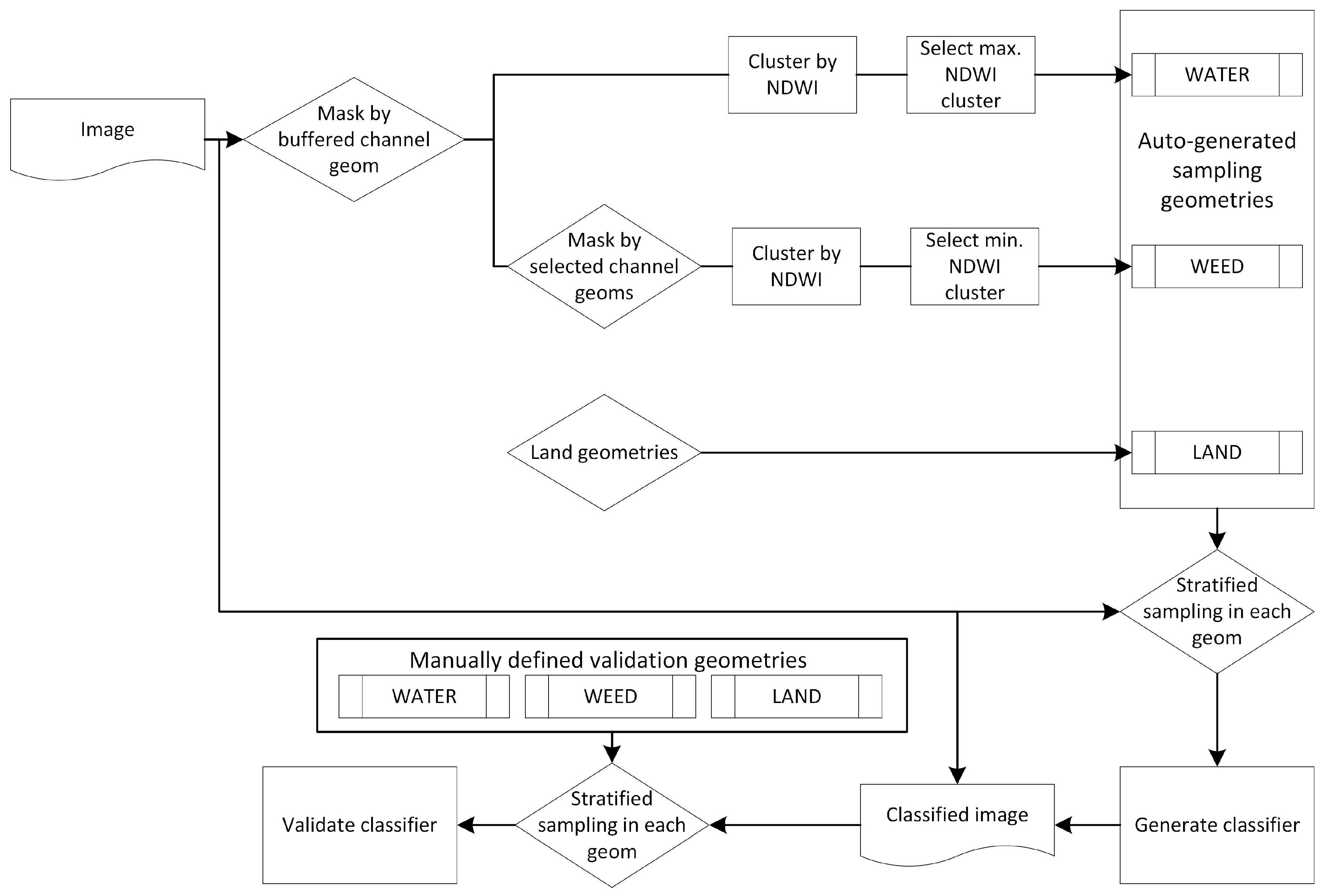
Clearly, a method is needed to enable robust classification of images that does not rely on users spending significant time drawing new polygons identifying classes for each new image. To this end, a semi-automatic method to re-train the classifier for each new image was developed using a combination of unsupervised and supervised classification. The unsupervised classification automatically finds geometries of water and weed to sample within to train the supervised classifier. The steps are as follows (illustrated in Figure 3):
- For land areas, a number of polygon geometries covering land areas around the edges of the channels are drawn. Land areas do not change with time, so they can be used for all new images. These areas were then used as the sampling geometries to generate training data for the land class.
- For water areas, clustering analysis (unsupervised classification) is used to automatically find areas of water in the image:
- –
- The clustering is performed using the band with best separability between the water class and the other classes. The K-Means clustering method implemented in GEE was used with three clusters.
- –
- The mean NDWI of each of the clusters is calculated (as NDWI was found to give the best separability between water and other classes, shown in Section 3.1.1 below). The cluster with the maximum NDWI is used as the sampling geometry to generate training data for the water class.
- To find weed areas, polygons were drawn covering only channel areas with reasonable distribution between water and weed (excluding land). These areas thus only contained water and weed. Clustering analysis was again performed on the NDWI of these channel areas with a similar method as that described above. The cluster with minimum NDWI was used as the sampling geometry to generate training data for the weed class.
This combination of unsupervised classification and supervised classification results in a robust and time-efficient method, where a new classifier is generated for each new image. The definition of training polygons is simple, as only polygons covering some of the land in an image, and some of the channel area in an image are needed. These same polygons can be used over multiple images of the same area in a time series, as the clustering automatically separates the water and weed areas for sampling (the user does not need to manually define weed/water areas for each new image).
To validate this classification procedure, manual validation geometries were drawn on selected images defining areas of land, water and weed. These geometries were separate to the land and channel polygons used for training the classifier to ensure fair assessment of classifier performance.
Validation is assessed for the main results using error matrices, as recommended in [25]. These matrices provide information on both omission errors (validation pixels that were not correctly classified to their true class) and commission errors (validation pixels that were incorrectly classified to another class). For some of the comparison results (comparing classifiers, resolutions, band inputs) where space would prohibit printing all the error matrices, the kappa value is used to provide a summary of the classification accuracy, as it includes information both of correctly and incorrectly assigned validation points [25]. Values of kappa over 0.75 are generally regarded as being indicative of excellent agreement between actual and predicted classes.
3. Results
3.1. Intensive Small Area Mapping by UAV
A time series of UAV images was used to assess the possibility of detecting weed change with time. The capture areas are shown in Figure 1. The capture dates and times are shown in Table 2.
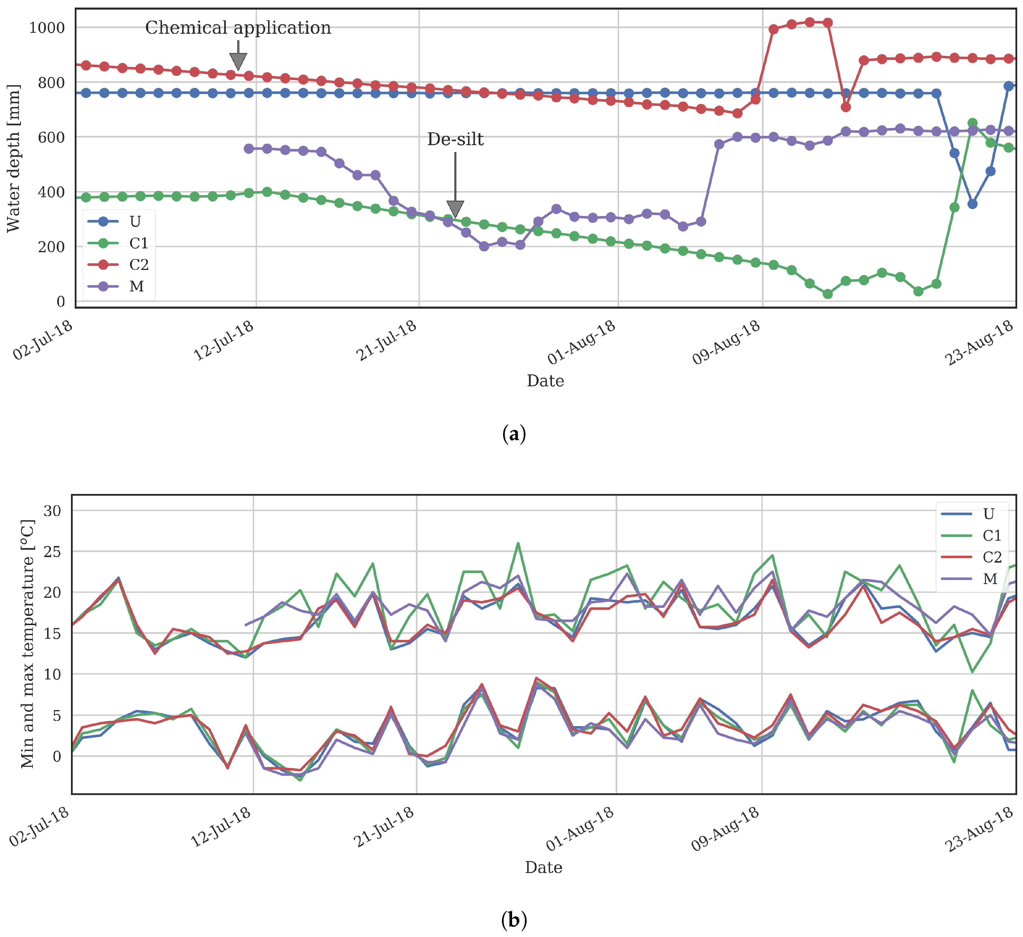
Throughout the study, WiField loggers collected water depth and temperature data, which is shown in Figure 4. Evaporation and leaking/seepage is indicated by smoothly declining water levels, as seen in the chemical treatment channels (C1 and C2). These channels were ’locked-up’ after chemical application with no water allowed back in during the treatment period. The untreated channel (U) was maintained at a constant water level by the automated channel control system, except towards the end of the study where it was drained and then refilled. The mechanical treatment channel (M) had low water levels while the de-silting was occurring, and was refilled shortly after.
The first image in the time series (2 July) from the C1 channel was used to assess class reflectances, and classifier accuracy with different bands, resolutions and classification algorithms. The selected parameters were then used on a time series of images from the U (untreated) channel to validate the classification method over numerous image dates. The validated method was then used over all the channels (U, M, C1 and C2) over the whole time series to assess changes in the weed area to compare the different weed control methods.
3.1.1. Reflectances of Each of the Classes
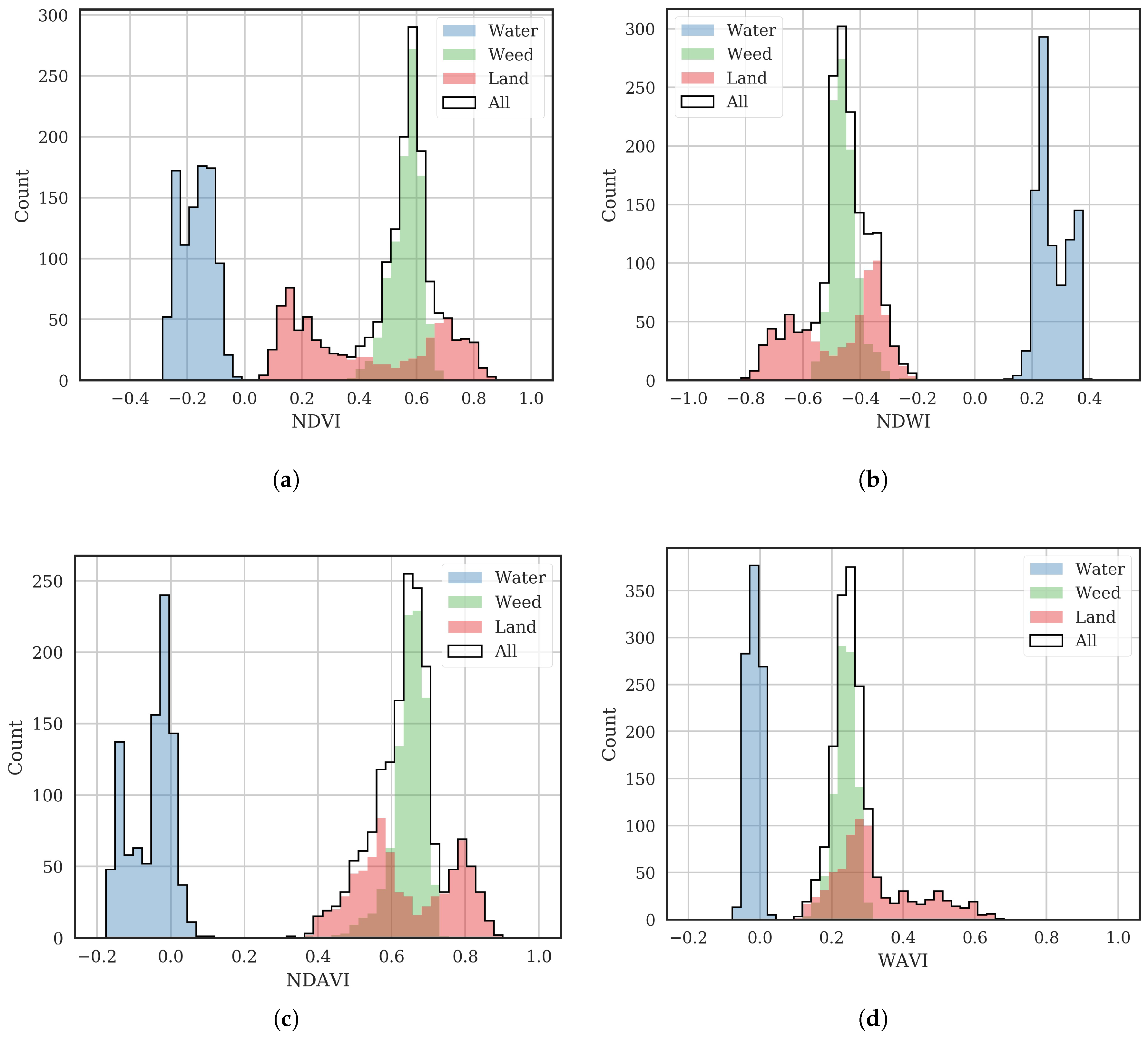
Geometries identifying areas of water, land and weed were drawn on the 2 July C1 image. The value of vegetation indices within each of these labelled geometries was sampled. A histogram of the reflectance values for significant vegetation indices is shown in Figure 5. This indicates the potential separability of each of the classes. Clearly, it is quite straightforward to separate water from land and/or weed using any of the indices shown. It is more difficult to separate weed and land. Land includes both unvegetated areas (bare soil, road, structures, etc.) and vegetation areas such as trees and other plants. This is the reason for the bi-modal distribution of the vegetation indices of the land classes.
These observations are quantified in Table 4, which shows the normalized mean distances (NMDs) between each of the classes. NDWI seems the best index to separate water from both land and weed, with NMDs of 7.38 and 14.46, respectively. This is why clustering can be used to robustly and automatically find water areas. The low NMDs for land-weed indicate a simple separation is not possible. The land area does not change between images in a time series, so can easily be defined by static geometries. There is good separability between weed and water classes, if land can be excluded. Thus, weed training areas can be defined by clustering defined channel geometries that include water and weed but not land. The best index for separating water and weed is again NDWI, with an NMD of 14.46 from Table 4.
These observations lead to the combined unsupervised (clustering) and supervised classification methodology described in Section 2.4.6 and diagrammed in Figure 3.
3.1.2. Classification Accuracy
Having devised the combined unsupervised-supervised classification method that is hypothesised to be robust, time-efficient and simple, the method is now assessed. First, different supervised classification algorithms are compared, then optimal combinations of image bands and indices input to the classifier are compared, and then the accuracy with a range of image resolutions are assessed.
For brevity, classification performance with different parameters will be compared with the kappa value, computed from the error matrices. An example is given from the 2 July image of the U channel. The selected optimum parameters found in the following sections are used (classification and regression tree (CART) classifier; 0.05 m resolution; and the red, green, blue and near-infrared bands). The error matrix is shown in Table 5. The matrix indicates that all 1000 samples from within the water validation geometry were classified correctly, 23 of the 1000 samples from within the land validation geometry were incorrectly classified as water and 24 were incorrectly classified as weed and so on. This error matrix has an overall accuracy of 0.983 (the sum of the diagonal divided by total observations), a consumers accuracy of [0.978,0.996,0.976] and a producers accuracy of [1,0.953,0.996]. The kappa value for this matrix is 0.974, indicative of excellent classifier accuracy.
3.1.3. Comparison of Classification Methods
GEE implements a range of classification algorithms. The accuracy of many of these was tested for this application, using the 2 July UAV image from the C1 channel. In each case, the default classification parameters were used. The kappa value results (calculated from the error matrices of actual vs. classified values) are shown in Table 6. It can be seen that the classification and regression tree (CART) classification performed the best. In the following sections, the CART classifier will be used.
3.1.4. Comparison of Classification Bands
Here, the optimal bands to train the classifier with are investigated, again for the 2 July image of the C1 channel. The MicaSense RedEdge camera has red, green, blue, red edge and near-infrared bands. In addition to the raw bands, the classifier was also trained with common indices which are computed from these bands. The results are in Table 7. The vegetation indices taken in isolation do not perform well, probably because of the overlap between land and weed vegetation indices as seen in Figure 5. Taking four raw bands (B, G, R, NIR) is optimal, and is used in the following investigations. The addition of the red edge band is not necessary for this application, but may be more important for higher dimensional classification (for example, to classify different weed species).
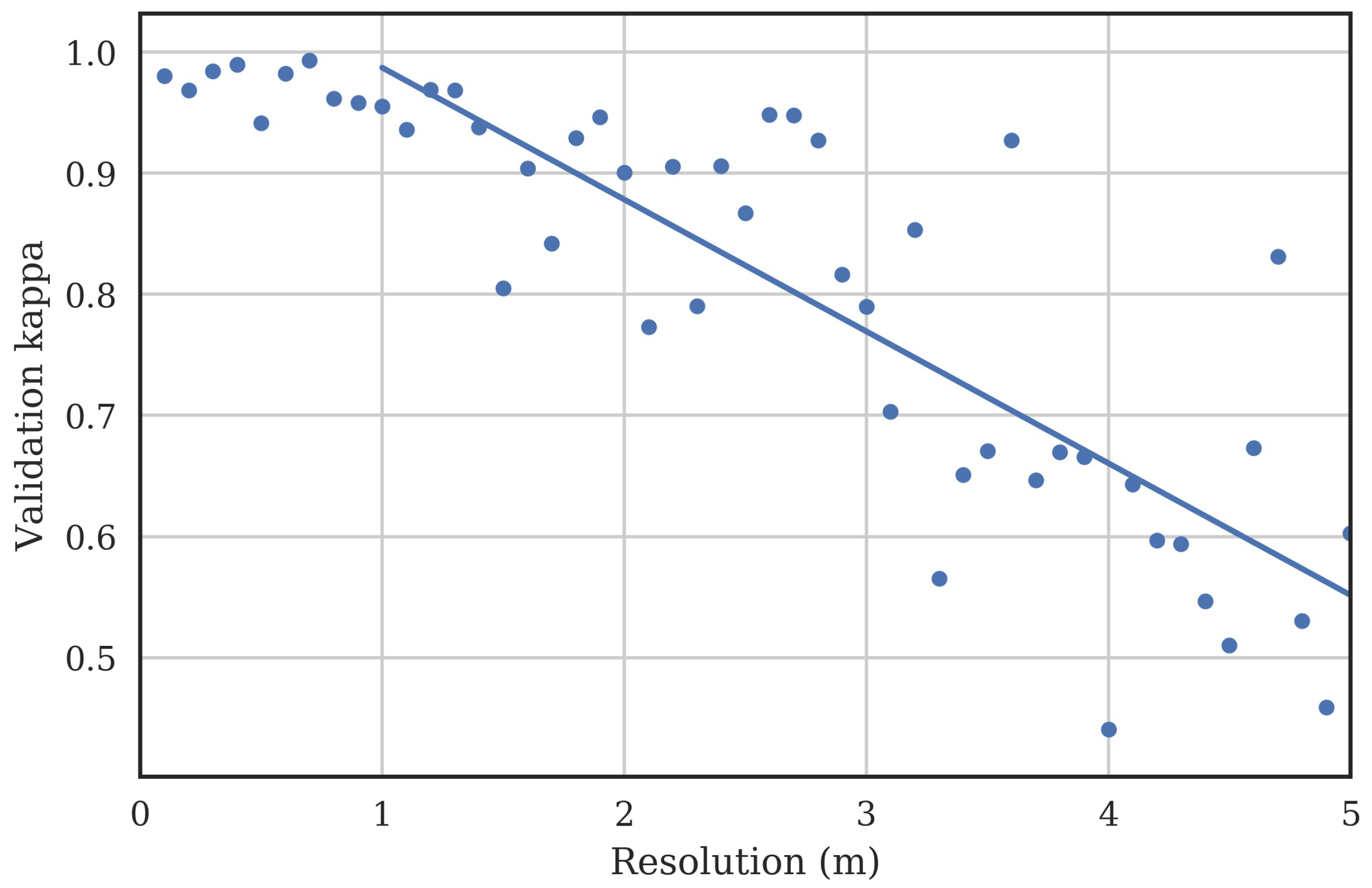
3.1.5. Comparison of Image Resolutions
In this section, the effect of image resolution is investigated for the 2 July image of the C1 channel. This is useful to find the minimum required image resolution to classify weed areas in irrigation channels. The UAV imagery had a native resolution of 0.05 m. The imagery was coarsened from 0.1 to 5 m using the GEE resample algorithm. The results are shown in Figure 6. It can be seen that classification accuracy is very good with resolutions less than 1 m. It drops off rapidly above this. This is intuitively expected, as the channel widths are less than 10 m, and weed areas are often small and isolated. The points in Figure 6 increasingly deviated from the line of best fit as pixel size increased. One reason for this is the training and validation sets became small, as there were limited pixels to sample within the validation geometries with large pixel sizes.
3.1.6. Validation over a Time Series of Images
Having assessed the classification method and parameters on a single image, its robustness over multiple images needs to be validated, as there may be different lighting conditions, water colour and turbidity, weed reflectances, etc. The untreated (U) channel was used for this purpose, as the land, weed and water areas did not change so the same validation geometries could be used for every image in the time series.
The validation kappa for each image is shown in Table 8. The kappa is lowest in the 23 August image. This image was taken just after the channel was drained and refilled as seen in Figure 4. A visual inspection of this image reveals that some of the weed patches had been either submerged or washed away, which together with the fact that the validation geometries were kept fixed for all images in the time series is the reason for the lower kappa for this image. However, it can be seen that the accuracy is excellent, with kappa remaining above 0.9 for all images over the two-month period.
3.1.7. Assessing Change in Weed Growth
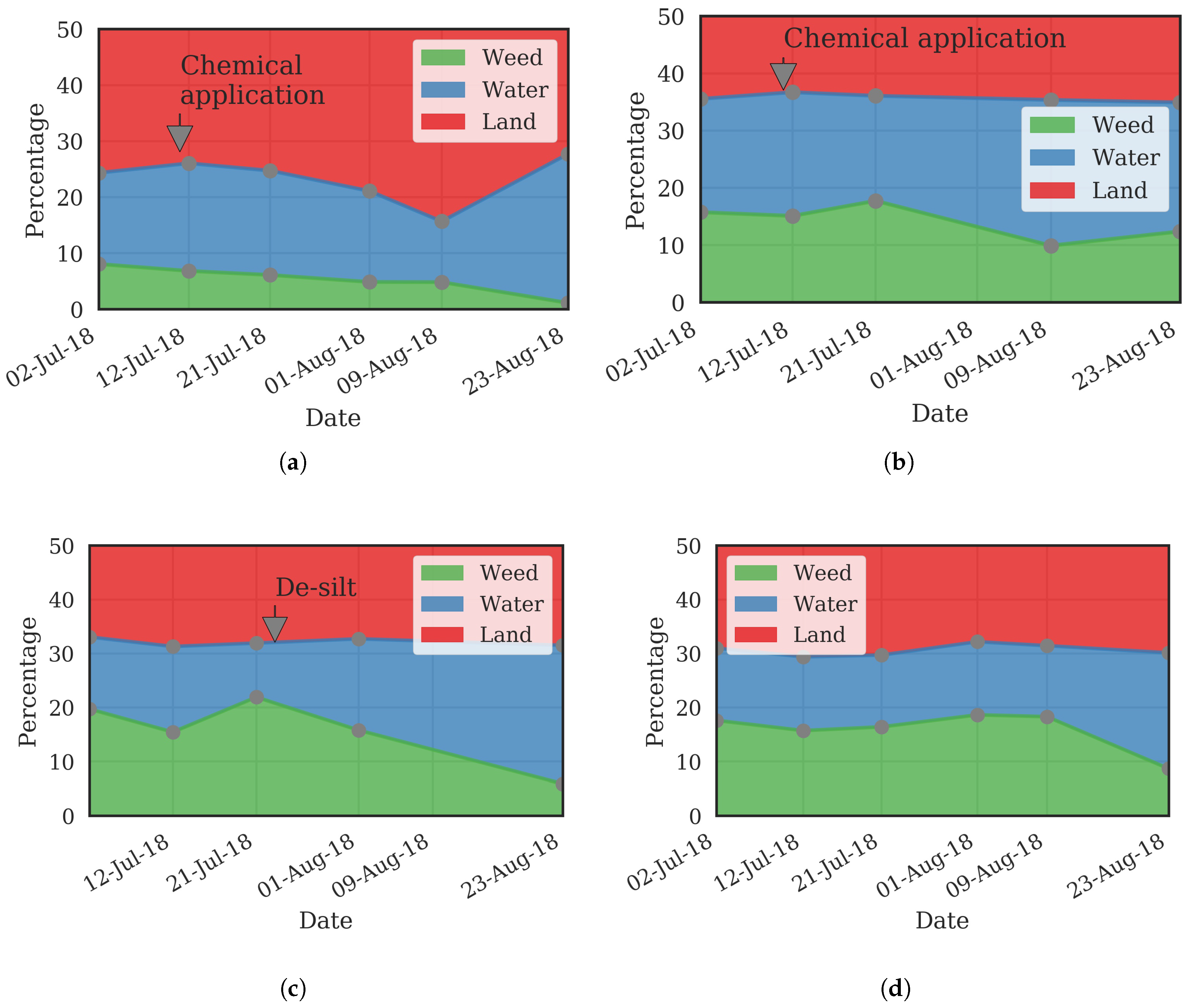
One application of irrigation channel weed mapping is assessing change in weed growth. This could indicate potential hot spots of growth that need controlling as soon as possible. It could also provide a method to assess the efficacy of different weed control methods, for example different chemical or mechanical controls. The long-term trends of weed growth could be analysed as a multi-year image database is built.
The four channels (Table 2) were imaged throughout the study period. The fixed training geometries for land and channel were defined for each of the channels. After classification, the area of each of the classes (water, land and weed) was computed. This could be used to indicate decline or growth of weeds. All this takes less than a minute in the GEE cloud computing environment. The results are shown in Figure 7. Note that these results are during the winter period, where there are a lot of dynamics in channels being drained and refilled, and weed control works being done. The characteristics are likely to not show as much variance during the peak irrigation season.
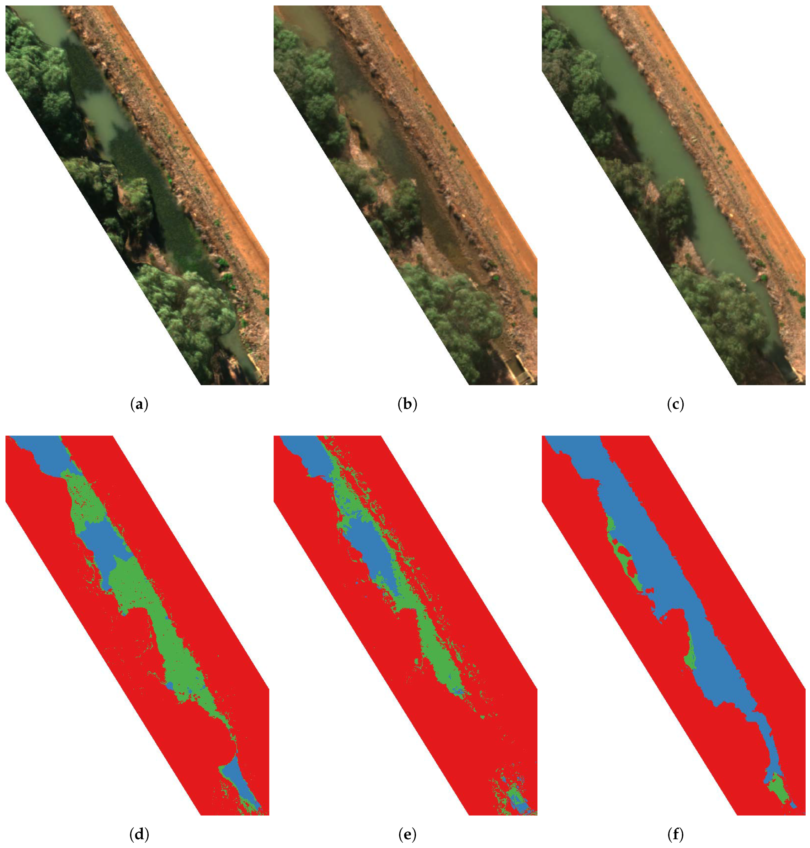
The visual and classified images from 2 July, 9 August and 23 August for the C1 channel are shown in Figure 8. Figure 7a shows the corresponding change in relative areas of land, water and weed for this channel. It is surprising to see the land area decline until 9 August, then rise again. The reason becomes clear when the water depth data in Figure 4 is examined. The water level dropped due to evaporation and leaking/seepage. On 11 August, areas of dry ground were visible. The channel was then refilled to more than its starting level on the 23 August image. There was little weed visible in the channel on this date, which is also correctly shown in both the percentage area graph and the classified image.
The other channels in Figure 7 show land area that is relatively constant, as the channels did not empty to the same extent as the C1 channel. In general, the weed area declines in the chemically and mechanically controlled channels (C1, C2 and M). In the untreated channel (U), the weed area is relatively constant (see Figure 7d). However, the 23 August image shows a lower weed area. This is for the reason discussed in Section 3.1.6—that the water level was dropped and refilled immediately prior to the image, leading to some of the weed patches becoming submerged on 23 August.
This section has shown the usefulness of using the developed classification method over a time-series of images of irrigation channels to monitor weed growth.
3.2. Large Area Mapping by Satellite
The methods developed above are now applied to much larger areas, using satellite images from the WorldView-3 constellation. Two images were purchased from different dates but covering the same 38.5 km area as described in Section 2.3.2.
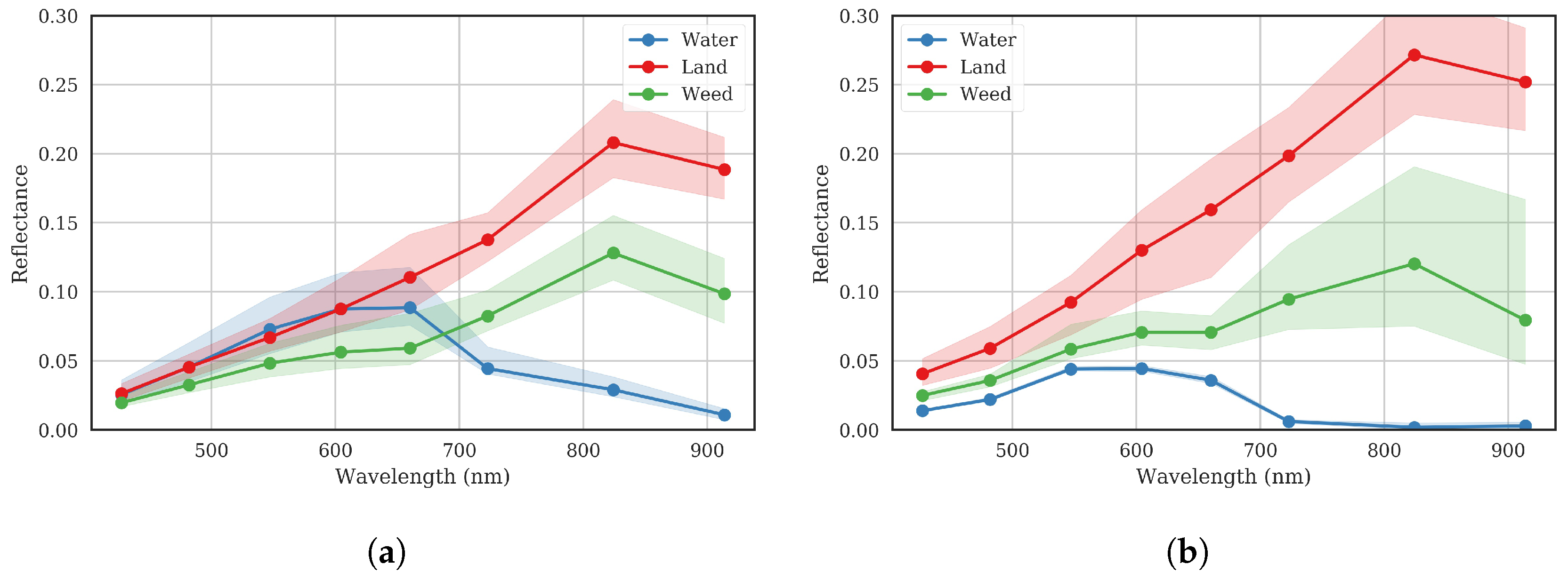
Separate geometries were drawn to mark out areas of land, water and weed in the 2017 and 2018 images. The image bands were sampled randomly within each of these polygons at a resolution of 0.3 m. The median, 25 and 75 percentiles for the 8-band reflectances of each of the classes for both images are shown in Figure 9. The 2017 image was on a day with wind coming from the Nor-Nor-East creating ripples aligning with the sun direction and thus creating reflections on the water. This explains the wider spread and different characteristics in the water reflectance in 2017 when compared with 2018. The 2017 image was taken in early autumn, whereas the 2018 image was from mid-summer with corresponding differences in vegetation on the land and weed in the channels. The variation in the reflectances of the classes over time is evident, again showing that a classifier generated from one image cannot be applied to accurately classify another image.
Next, the automated unsupervised-supervised classification method (Section 2.4.6) was applied. The same land and channel training geometries were used for both image dates. Separate validation geometries were used (as weed areas were different from 2017 to 2018). The resulting error matrices are shown in Table 9. Kappa remains above 0.85 for both images, indicating excellent accuracy.
The classified areas for each of the classes from the two images are shown in Table 10. The total area classified is 0.614 km of the total satellite image size of 38.5 km, which consists of 20 m wide strips around the supply channels. The total length of channels mapped is then 30.7 km. The last column shows the proportion of the total channel area (weed + water) that is taken up by weed. The similarity in the land area between the two images verifies that this area is being classified correctly, as it does not change from image to image. The percentage of weed information will be very useful for irrigation network companies to track the weed status of their channels through the season, and from season to season. The classification and result calculations of these large high-resolution images took seconds in GEE.
4. Discussion
This study has demonstrated the potential for the use of remote sensing to monitor vegetation in irrigation channel networks, which is a major cause of impeded flow rates. GEE was used to process, analyse and classify UAV and satellite images in seconds.
UAV and satellite imagery each have their benefits. Data from UAVs are useful for intensive monitoring of small areas of channels with high resolution. They offer a relatively low cost way of mapping stretches of channel, with the typical time taken to set up and capture a stretch of 1 km being about 1 h. Applications for this include intensive experiments to assess the effectiveness of weed control methods (chemical or mechanical), which require a time series of images to analyse change. Purchasing satellite images over small experimental areas and multiple dates would not be cost effective. Use of UAVs also provides very high resolution, which may be needed for deeper classification than was performed in this study, such as classifying between species of weeds. UAVs will also be useful to check for critical stretches of channel at short notice. An example where this is useful is when a farmer complains that the promised water delivery rates are not being met, a UAV could be used to survey the channels leading to the farm to determine if weed is the reason for the constraint, and the water delivery provider could then quickly make a decision on how to rectify the issue.
Satellite imagery will be important to monitor the large areas covered by the entire irrigation channel networks. It is clear that the resolution of current free satellite imagery is not sufficient. For example, the Sentinel constellation resolution is 10 m, which is not useful in monitoring channels with widths of much less than 10 m. Thus, images must be purchased, in order to obtain resolutions of 1 m or better. Images should contain at least the red, green, blue and near-infrared bands. Satellite images could be obtained for a few key times in the year. For example, one in the off-season could be used to plan weed control when it is possible to dry down channels and to target intensive work on problem areas. An image immediately preceding the peak irrigation season could be used to ensure the network is ready to deliver high flows to all areas and any last minute rectification of weed issues could be performed. An image in the midst of the peak irrigation season could be used to identify problem areas that are causing impeded flows. As a database of multi-season images are built up, trends in weed growth and problem areas could be identified and the reasons for proliferation of weeds in certain areas investigated and resilience against weed outbreaks improved. Multi-season images will also allow tracking of the proliferation of introduced species, which may be resistant to current weed control strategies.
The satellite images used in this study were very high resolution 8-band images, which comes with a high price. The minimum requirements for satellite images for weed area identification should be determined to reduce costs. Example satellite image costs are shown in Table 11.
To compare the cost of surveying the network by satellite, to manually survey with a person in a car, the length of the supply networks for a number of rectangular areas within Figure 1 was determined. The length of channels was found to be roughly proportional to the square root of the area: . Thus, for a 500 km area, the length of channel is about 550 km. If 1.5 m resolution satellite images are determined to be sufficient, the cost for an image will be around 500 × 6 = $3000 (Table 11). If a manual survey is done, assuming a 10 km/h driving speed, the cost is the hourly rate for a driver/surveyor multiplied by the time, plus the mileage costs for the car. Assuming an hourly rate (including tax, superannuation and insurance) of $100/h, and mileage costs of $1/km, the cost to manually survey the area would be 100 × 550/10 + 550 = $6050, approximately twice that of the satellite image. This simple analysis shows that replacing manual monitoring with satellite monitoring is an attractive option. Satellite monitoring also provides additional benefits such as quantifiable weed area calculations and regular mapping of the region. Additional value could be generated from the purchased images by using them for other purposes, such as finding NDVI to determine the total area of irrigated land in a given season.
Future work will involve investigating the benefits that hyperspectral data may bring to the task of weed identification. Hyperspectral data has more bands and therefore may be able to separate the classes more precisely, particularly considering the different reflectance signatures of weed and land vegetation species [15]. The World-View 3 data has eight bands, of which only four were used in this study. The possibility of classifying between species will be useful as different weeds are more responsive to different methods of control. Higher resolution imagery may also be needed so that object- and texture-based classification methods can be employed [16].
Recent work has shown the strong impact of anisotropic reflectance of mixed vegetation and water environments [27]. The electromagnetic reflectance environment of irrigation channels is complex, (with interactions between solar radiation, vegetation canopy, water surface, water column, and channel bottom), and the use of radiative transfer models of the system to obtain bidirectional reflectance functions may enhance classification accuracy [28]. More work is needed in this area.
As a larger database of images of the channels are built over a longer time scale, with more variance in reflectance characteristics of each of the classes, it will be useful to investigate if a single classifier can be trained that is robust against all images. The classifier could be updated as new images become available. It would also be useful to investigate the possible merging of classifiers for UAV and satellite-based images, which may involve some radiometric correction as the instrument bands are different, as seen in Table 1. Other future work could involve applying the techniques developed here to other regions, and assess how robust the method of weed detection is with different species of weeds that are predominant in those areas.
5. Conclusions
Weed growth in irrigation network channels is a major source of flow constraint, which results in slow delivery of irrigation water to farms. This paper has demonstrated the use of remotely sensed multispectral images from UAV and satellite platforms to detect and quantify areas of weed in irrigation network channels. An algorithm was developed, combining unsupervised and supervised classification to robustly identify areas of weed, water and land from images with very little user intervention or overhead in supplying training data for new images. Classification accuracy typically achieved kappa values of greater than 0.85. The required bands to achieve these results were red, green, blue and near-infrared, and resolutions of better than one metre were recommended. UAV images were shown to be useful for intensively monitoring small areas of irrigation channels over time, for example, to quantify the change in weed after chemical or mechanical controls are implemented. Satellite images were processed over very large areas and the total area of weed in the channels throughout the images were automatically calculated. These techniques will facilitate improvement in the maintenance of timely water delivery from irrigation channel networks.
Author Contributions
J.B. performed the image capture, analysed the data and prepared the manuscript. J.L.B. wrote the section on vegetation and provided advice on weed types. J.H. provided overall project guidance.
Funding
This research was funded by Murrumbidgee Irrigation, Ltd. (Griffith 2680, Australia).
Acknowledgments
The authors thank Lindsay Golsby-Smith, Jeff Shaw, Anthony Gulloni, Pieter van der Merwe and Brett Jones from Murrumbidgee Irrigation, Ltd. (Griffith 2680, Australia) for providing advice and data.
Conflicts of Interest
The authors declare no conflict of interest.
References
- Wahlin, B.; Zimbelman, D. Canal Automation for Irrigation Systems: American Society of Civil Engineers Manual of Practice Number 131. Irrig. Drain. 2018, 67, 22–28. [Google Scholar] [CrossRef]
- Dugdale, T.M.; Hunt, T.D.; Clements, D. Aquatic weeds in Victoria: Where and why are they a problem, and how are they being controlled? Plant Protect. Q. 2013, 28, 35. [Google Scholar]
- Bakry, M.F.; Gates, T.K.; Khattab, A.F. Field-measured hydraulic resistance characteristics in vegetation-infested canals. J. Irrig. Drain. Eng. 1992, 118, 256–274. [Google Scholar] [CrossRef]
- MI. Murrumbidgee Irrigation Company Overview. 2018. Available online: http://www.mirrigation.com.au/ArticleDocuments/199/Fact%20Sheet%20Company%20Overview.pdf.aspx (accessed on 22 May 2018).
- Sabol, B.M.; Melton, R.E.; Chamberlain, R.; Doering, P.; Haunert, K. Evaluation of a digital echo sounder system for detection of submersed aquatic vegetation. Estuaries 2002, 25, 133–141. [Google Scholar] [CrossRef]
- Vis, C.; Hudon, C.; Carignan, R. An evaluation of approaches used to determine the distribution and biomass of emergent and submerged aquatic macrophytes over large spatial scales. Aquat. Bot. 2003, 77, 187–201. [Google Scholar] [CrossRef]
- Goddijn-Murphy, L.; Dailloux, D.; White, M.; Bowers, D. Fundamentals of in situ digital camera methodology for water quality monitoring of coast and ocean. Sensors 2009, 9, 5825–5843. [Google Scholar] [CrossRef] [PubMed]
- Silva, T.S.F.; Costa, M.P.F.; Melack, J.M.; Novo, E.M.L.M. Remote sensing of aquatic vegetation: theory and applications. Environ. Monit. Assess. 2008, 140, 131–145. [Google Scholar] [CrossRef] [PubMed]
- Villa, P.; Bresciani, M.; Braga, F.; Bolpagni, R. Comparative assessment of broadband vegetation indices over aquatic vegetation. IEEE J. Sel. Top. Appl. Earth Obs. Remote Sens. 2014, 7, 3117–3127. [Google Scholar] [CrossRef]
- Cho, H.J.; Lu, D. A water-depth correction algorithm for submerged vegetation spectra. Remote Sens. Lett. 2010, 1, 29–35. [Google Scholar] [CrossRef] [Green Version]
- Visser, F.; Buis, K.; Verschoren, V.; Meire, P. Depth estimation of submerged aquatic vegetation in clear water streams using low-altitude optical remote sensing. Sensors 2015, 15, 25287–25312. [Google Scholar] [CrossRef] [PubMed]
- Göktoǧan, A.H.; Sukkarieh, S.; Bryson, M.; Randle, J.; Lupton, T.; Hung, C. A rotary-wing unmanned air vehicle for aquatic weed surveillance and management. J. Intell. Robot. Syst. 2010, 57, 467. [Google Scholar] [CrossRef]
- Chabot, D.; Dillon, C.; Ahmed, O.; Shemrock, A. Object-based analysis of UAS imagery to map emergent and submerged invasive aquatic vegetation: A case study. J. Unmanned Veh. Syst. 2016, 5, 27–33. [Google Scholar] [CrossRef]
- Rendong, L.; Jiyuan, L. Estimating wetland vegetation biomass in the Poyang Lake of central China from Landsat ETM data. IEEE Geosci. Remote Sens. Sympos. 2004, 7, 4590–4593. [Google Scholar]
- Adam, E.; Mutanga, O.; Rugege, D. Multispectral and hyperspectral remote sensing for identification and mapping of wetland vegetation: A review. Wetlands Ecol. Manag. 2010, 18, 281–296. [Google Scholar] [CrossRef]
- Husson, E.; Ecke, F.; Reese, H. Comparison of manual mapping and automated object-based image analysis of non-submerged aquatic vegetation from very-high-resolution UAS images. Remote Sens. 2016, 8, 724. [Google Scholar] [CrossRef]
- Fyfe, S.K. Spatial and temporal variation in spectral reflectance: Are seagrass species spectrally distinct? Limnol. Oceanogr. 2003, 48, 464–479. [Google Scholar] [CrossRef] [Green Version]
- Gorelick, N.; Hancher, M.; Dixon, M.; Ilyushchenko, S.; Thau, D.; Moore, R. Google Earth Engine: Planetary-scale geospatial analysis for everyone. Remote Sens. Environ. 2017. [Google Scholar] [CrossRef]
- Sainty, G.R.; Jacobs, S.W. Waterplants of New South Wales. New South Wales Water Resour. Commiss. 1981, 7, 550. [Google Scholar]
- Brinkhoff, J.; Hornbuckle, J. WiField, an IEEE 802.11-based Agricultural Sensor Data Gathering and Logging Platform. In Proceedings of the 11th International Conference on Sensing Technology, Sydney, Australia, 4–6 December 2017. [Google Scholar]
- DigitalGlobe. Absolute Radiometric Calibration: 2016v0. 2017. Available online: https://dg-cms-uploads-production.s3.amazonaws.com/uploads/document/file/209/ABSRADCAL_FLEET_2016v0_Rel20170606.pdf (accessed on 6 June 2018).
- Chavez, P.S., Jr. An improved dark-object subtraction technique for atmospheric scattering correction of multispectral data. Remote Sens. Environ. 1988, 24, 459–479. [Google Scholar] [CrossRef]
- Gitelson, A.A.; Kaufman, Y.J.; Stark, R.; Rundquist, D. Novel algorithms for remote estimation of vegetation fraction. Remote Sens. Environ. 2002, 80, 76–87. [Google Scholar] [CrossRef] [Green Version]
- Ward, D.; Hamilton, S.; Jardine, T.; Pettit, N.; Tews, E.; Olley, J.; Bunn, S. Assessing the seasonal dynamics of inundation, turbidity, and aquatic vegetation in the Australian wet–dry tropics using optical remote sensing. Ecohydrology 2013, 6, 312–323. [Google Scholar] [CrossRef]
- Congalton, R.G. A review of assessing the accuracy of classifications of remotely sensed data. Remote Sens. Environ. 1991, 37, 35–46. [Google Scholar] [CrossRef]
- LandInfo. Buying Satellite Imagery: Pricing Information for High Resolution Satellite Imagery. Available online: http://www.landinfo.com/satellite-imagery-pricing.html (accessed on 21 June 2018).
- Sun, T.; Fang, H.; Liu, W.; Ye, Y. Impact of water background on canopy reflectance anisotropy of a paddy rice field from multi-angle measurements. Agric. For. Meteorol. 2017, 233, 143–152. [Google Scholar] [CrossRef]
- Zhou, G.; Niu, C.; Xu, W.; Yang, W.; Wang, J.; Zhao, H. Canopy modeling of aquatic vegetation: a radiative transfer approach. Remote Sens. Environ. 2015, 163, 186–205. [Google Scholar] [CrossRef]
Figure 1.
(a) a portion of the Murrumbidgee Irrigation Area with imagery from the Sentinel-2 constellation from 1 Jan 2018. The supply channels are shown in blue. The areas mapped by the UAV and satellite are shown; (b) one of the WorldView-3 satellite images; (c) UAV image of the untreated (U) channel.

Figure 2.
Common weed types in the MIA channels (a) Ribbonweed; (b) Pondweed; (c) Parrot’s feather and cumbungi.
Figure 2.
Common weed types in the MIA channels (a) Ribbonweed; (b) Pondweed; (c) Parrot’s feather and cumbungi.

Figure 3.
Method of generating a classified image from a satellite image. The land and selected channel geometries are constant across images, so a new classifier is generated for each image without a user needing to manually define new water, land and weed polygons.
Figure 3.
Method of generating a classified image from a satellite image. The land and selected channel geometries are constant across images, so a new classifier is generated for each image without a user needing to manually define new water, land and weed polygons.

Figure 4.
Logger data from each of the sites. (a) water depth with dates on which UAV images were taken indicated with vertical lines; (b) the minimum and maximum daily air temperatures.
Figure 4.
Logger data from each of the sites. (a) water depth with dates on which UAV images were taken indicated with vertical lines; (b) the minimum and maximum daily air temperatures.

Figure 5.
Vegetation index histograms for each of the classes for the 2 July image of the C1 channel. (a) NDVI. (b) NDWI. (c) NDAVI. (d) WAVI.
Figure 5.
Vegetation index histograms for each of the classes for the 2 July image of the C1 channel. (a) NDVI. (b) NDWI. (c) NDAVI. (d) WAVI.

Figure 6.
Classification validation accuracy kappa for identifying the water, land and weed classes as a function of the image resolution.
Figure 6.
Classification validation accuracy kappa for identifying the water, land and weed classes as a function of the image resolution.

Figure 7.
Area of each of the classes over time for the four channels mapped with the UAV. (a) C1; (b) C2; (c) M; (d) U.
Figure 7.
Area of each of the classes over time for the four channels mapped with the UAV. (a) C1; (b) C2; (c) M; (d) U.

Figure 8.
The (a) first, (b) fifth, and (c) sixth images from the time series UAV images of the C1 channel (small portion shown). The corresponding classified results for the (d) first, (e) fifth, and (f) sixth images are shown in the bottom row, with blue = water, red = land and green = weed.
Figure 8.
The (a) first, (b) fifth, and (c) sixth images from the time series UAV images of the C1 channel (small portion shown). The corresponding classified results for the (d) first, (e) fifth, and (f) sixth images are shown in the bottom row, with blue = water, red = land and green = weed.

Figure 9.
Reflectances of samples from each of the defined class polygons in the WorldView-3 images. The lines shows the median reflectances and the shaded areas the 25–75th percentiles. (a) 2017 image; (b) 2018 image.
Figure 9.
Reflectances of samples from each of the defined class polygons in the WorldView-3 images. The lines shows the median reflectances and the shaded areas the 25–75th percentiles. (a) 2017 image; (b) 2018 image.


Table 1.
Specifications of the utilised bands of the MicaSense RedEdge UAV-mounted camera, and the World-View 3 satellite instrument.
Table 1.
Specifications of the utilised bands of the MicaSense RedEdge UAV-mounted camera, and the World-View 3 satellite instrument.
| Band | MicaSense RedEdge | World-View 3 | ||
|---|---|---|---|---|
| Center (nm) | Bandwidth (nm) | Center (nm) | Bandwidth (nm) | |
| Blue | 475 | 20 | 481.9 | 40.5 |
| Green | 560 | 20 | 547.1 | 61.8 |
| Red | 668 | 10 | 660.1 | 58.5 |
| Near-infrared | 840 | 40 | 824.0 | 100.4 |
Table 2.
Channels used for UAV image captures, the approximate total image area captured, and the dates and times of the captures (all in 2018).
Table 2.
Channels used for UAV image captures, the approximate total image area captured, and the dates and times of the captures (all in 2018).
| Channel | Length | Width | Area | Treatment | 2 July | 12 July | 21 July | 1 August | 9 August | 23 August |
|---|---|---|---|---|---|---|---|---|---|---|
| U | 500 m | 5 m | 50,000 m | Untreated | 14:00 | 13:20 | 13:20 | 13:40 | 13:20 | 13:50 |
| C1 | 1200 m | 4 m | 120,000 m | Chemical | 13:40 | 13:00 | 13:00 | 13:20 | 12:50 | 13:30 |
| C2 | 1200 m | 7 m | 120,000 m | Chemical | 13:00 | 13:40 | 13:50 | 13:30 | 13:10 | |
| M | 1200 m | 7 m | 120,000 m | Mechanical | 13:30 | 14:00 | 14:30 | 14:30 | 12:50 |
Table 3.
Vegetation index definitions, where B, R, G and are blue, red, green and near-infrared reflectance respectively, and .
Table 3.
Vegetation index definitions, where B, R, G and are blue, red, green and near-infrared reflectance respectively, and .
| NDVI | Normalized Difference Vegetation Index | |
| VARI | Visible Atmospherically Resistant Index | |
| NDWI | Normalized Difference Water Index | |
| NDAVI | Normalized Difference Aquatic Vegetation Index | |
| WAVI | Water Adjusted Vegetation Index | |
| SAVI | Soil Adjusted Vegetation Index | |
| EVI | Enhanced Vegetation Index |
Table 4.
Normalized mean distances (NMDs) between the classes for each vegetation index.
| Class NMD | NDVI | NDWI | NDAVI | WAVI | VARI | EVI | SAVI |
|---|---|---|---|---|---|---|---|
| Water-Land | 3.95 | 7.38 | 7.34 | 4.87 | 1.86 | 3.10 | 3.43 |
| Water-Weed | 13.57 | 14.46 | 13.55 | 10.30 | 1.03 | 10.40 | 10.89 |
| Land-Weed | 0.93 | 0.26 | 0.11 | 1.14 | 2.15 | 0.18 | 0.15 |
Table 5.
Error matrix for the 2 July untreated channel (U) image using optimum classification parameters.
Table 5.
Error matrix for the 2 July untreated channel (U) image using optimum classification parameters.
| Predicted | ||||
|---|---|---|---|---|
| Water | Land | Weed | ||
| Actual | Water | 1000 | 0 | 0 |
| Land | 23 | 953 | 24 | |
| Weed | 0 | 4 | 996 | |
Table 6.
Classifier accuracy for different classifiers using the kappa value.
| Classifier | Kappa |
|---|---|
| Minimum Distance | 0.91 |
| Support Vector Machine | 0.91 |
| Random Forest | 0.93 |
| Naive Bayes | 0.95 |
| Classification And Regression Tree | 0.98 |
Table 7.
Classifier accuracy with different input image band combinations.
| Classification Bands | Kappa |
|---|---|
| VARI | 0.48 |
| WAVI | 0.54 |
| NDAVI | 0.54 |
| NDWI | 0.71 |
| NDVI | 0.78 |
| R, G, B | 0.92 |
| NDWI, NDAVI, NDVI, VARI | 0.95 |
| NDVI, NDWI | 0.96 |
| R, G, B, RE, NIR | 0.98 |
| R, G, B, NIR | 0.98 |
Table 8.
Classifier accuracy for a time series of images over the untreated (U) untreated channel.
| Image Date | Kappa |
|---|---|
| 2 July 2018 | 0.98 |
| 12 July 2018 | 0.98 |
| 21 July 2018 | 0.98 |
| 1 August 2018 | 0.99 |
| 9 August 2018 | 0.98 |
| 23 August 2018 | 0.92 |
Table 9.
Classifier validation error matrices for the WorldView-3 images using automated classifier training method. (a) 2017 image, ; (b) 2018 image, .
Table 9.
Classifier validation error matrices for the WorldView-3 images using automated classifier training method. (a) 2017 image, ; (b) 2018 image, .
| (a) | ||||
|---|---|---|---|---|
| Predicted | ||||
| Water | Land | Weed | ||
| Actual | Water | 988 | 0 | 12 |
| Land | 1 | 869 | 33 | |
| Weed | 61 | 184 | 771 | |
| (b) | ||||
| Predicted | ||||
| Water | Land | Weed | ||
| Actual | Water | 1000 | 0 | 0 |
| Land | 0 | 857 | 46 | |
| Weed | 84 | 52 | 857 | |
Table 10.
Classification areas in km, and proportion of weed in the channels, from the WorldView-3 images.
Table 10.
Classification areas in km, and proportion of weed in the channels, from the WorldView-3 images.
| Image | Water (km) | Land (km) | Weed (km) | Weed (%) |
|---|---|---|---|---|
| 2017 | 0.155 | 0.364 | 0.095 | 38.0 |
| 2018 | 0.131 | 0.372 | 0.111 | 45.9 |
Table 11.
Satellite constellations and approximate costs for four-band tasked images [26].
Table 11.
Satellite constellations and approximate costs for four-band tasked images [26].
| Constellation | Resolution (m) | Cost ($US/km) | Minimum Area (km) |
|---|---|---|---|
| Sentinel | 10 | 0 | NA |
| Rapid Eye | 5 | <2 | 500 |
| SPOT6/7 | 1.5 | <6 | 500 |
| WorldView | 0.5 | <30 | 100 |
| WorldView | 0.3 | >30 | 100 |
© 2018 by the authors. Licensee MDPI, Basel, Switzerland. This article is an open access article distributed under the terms and conditions of the Creative Commons Attribution (CC BY) license (http://creativecommons.org/licenses/by/4.0/).
Share and Cite
MDPI and ACS Style
Brinkhoff, J.; Hornbuckle, J.; Barton, J.L. Assessment of Aquatic Weed in Irrigation Channels Using UAV and Satellite Imagery. Water 2018, 10, 1497. https://doi.org/10.3390/w10111497
AMA Style
Brinkhoff J, Hornbuckle J, Barton JL. Assessment of Aquatic Weed in Irrigation Channels Using UAV and Satellite Imagery. Water. 2018; 10(11):1497. https://doi.org/10.3390/w10111497
Chicago/Turabian StyleBrinkhoff, James, John Hornbuckle, and Jan L. Barton. 2018. "Assessment of Aquatic Weed in Irrigation Channels Using UAV and Satellite Imagery" Water 10, no. 11: 1497. https://doi.org/10.3390/w10111497
Note that from the first issue of 2016, this journal uses article numbers instead of page numbers. See further details here.