Numerical Analysis on the Hydrodynamic Performance of an Artificially Ventilated Surface-Piercing Propeller


College of Shipbuilding Engineering, Harbin Engineering University, Harbin 150001, China
*
Author to whom correspondence should be addressed.
Water 2018, 10(11), 1499; https://doi.org/10.3390/w10111499
Submission received: 11 September 2018
/
Revised: 18 October 2018
/
Accepted: 18 October 2018
/
Published: 23 October 2018
(This article belongs to the Special Issue Advances in Hydraulics and Hydroinformatics)
Abstract
:When operated under large water immersion, surface piercing propellers are prone to be in heavy load conditions. To improve the hydrodynamic performance of the surface piercing propellers, engineers usually artificially ventilate the blades by equipping a vent pipe in front of the propeller disc. In this paper, the influence of artificial ventilation on the hydrodynamic performance of surface piercing propellers under full immersion conditions was investigated using the Computational Fluid Dynamics (CFD) method. The numerical results suggest that the effect of artificial ventilation on the pressure distribution on the blades decreases along the radial direction. And at low advancing speed, the thrust, torque as well as the efficiency of the propeller are smaller than those without ventilation. However, with the increase of the advancing speed, the efficiency of the propeller rapidly increases and can be greater than the without-ventilation case. The numerical results demonstrates the effectiveness of the artificial ventilation approach for improving the hydrodynamic performance of the surface piercing propellers for high speed planning crafts.
1. Introduction
Surface-piercing propellers (SPPs) are also known as Surface penetrating propellers. The SPP is so named because part of the propeller is above the water surface and the rest is under the water during normal operation. Compared with the conventional propellers, the SPPs mainly have the following three advantages (Ding et al. [1]): (1) the resistance of the appendages, such as the paddle shaft and the shaft bracket, is minimized; (2) propeller diameter is no longer limited by some parameters such as soak depth and stern frame; and (3) the cavitation erosion on the blade surface is substantially reduced. Due to these advantages, the SPPs become an optimal choice for high-speed boats and some shallow draft ships, and thus have really good application prospects.
However, in some cases the SPPs might be operated under the large water immersion, e.g., the boats are at the bow-up status, which makes the SPPs be in heavy load conditions. One of the practical approaches to solve this problem is setting an aeration pipe in front of SPPs to ventilate the blades. This approach has been adopted in some actual boats and achieved significant results. Nonetheless, few attentions have been paid on how the ventilation of blades improves the hydrodynamic characteristics of SPPs. To this end, this paper is dedicated to investigate the influence of the ventilation of blades on the hydrodynamic performance of SPPs using numerical methods.
In some simplified studies, the surface-piercing process of an SPP blade can be deemed as the water-entry process of a 2D profile, which is easy to be understood. Zhao et al. [2] used the non-linear boundary element method to investigate the characteristics of the sprays generated by the water-entry of wedges with different bottom-angles. It was found that the increase of the wetted area directly leads to a great slamming pressure on the wetted surface. And when the slope angle of the bottom is larger than 30°, there is no typical slamming pressure concentration phenomenon due to the smaller wetted surface. Young et al. [3], in his doctoral dissertation, carried out similar studies on the water-entry of wedges, and analyzed the pressure distribution on the wetted surface of a flat plate under different entry angles.
Yari et al. [4] conducted a preliminary study on a wedge entering the water under different inclination angles. The obtained pressure distribution, free surface deformation, and so on agree well with the experimental data. Yu et al. [5] carried out a numerical study on the water entry problem of a 2D cross-section profile, and found that the cup shape of the trailing edge can enhance the hydrodynamic load on the edge, while reducing the lift-to-drag ratio as well as the efficiency of the propeller.
Ghassemi et al. [6] investigated the hydrodynamics of SPPs named SPP-1 and SPP-2 under full and half immersed conditions using a boundary element method (BEM). The numerical results agree well with experimental ones. In the study, they found that the Weber number has significant influence on the ventilation status of the SPP. Kinnas et al. [7] studied the bubble flow around the hydrofoil and SPPs using a BEM, in which they investigated the hydrodynamic effects of the bubble flow on the hydrofoil and SPPs with various blade profiles. Young et al. [8,9] carried out a series of studies on large-scale SPPs and super-vacuum paddles also by using the BEM, which contributed to the knowledge of the hydrodynamics of these propellers.
With the development of the computer technology, the CFD methods become popular and play the role of benchmark in the numerical studies on surface-piercing propellers. Young et al. [3] predicted the hydrodynamic performance of large-scale surface paddles using a coupled boundary element method–finite element method (BEM–FEM), and found that the numerical results compared well with those obtained by the Reynolds Averaged Navier–Stokes (RANS) solver (Fluent software), in which the Reynolds stress tensor was modeled using the SST form of the turbulence model. Shi et al. [10] investigated the wake of surface-piercing propellers, as well as the pulsating pressure on the paddles and the deformation of the free surface after the paddles. Alimirzazadeh et al. [11] employed the OpenFOAM software to study the hydrodynamic performance of SPP-841B surface paddle under different sway angles and immersion depths. In the study, the based Shear Stress Transport (SST) model with automatic wall functions (mixed formulation) was employed. The numerical results agree with experimental ones well under different immersion depths, while poorly under different sway angles. They found that increasing the yaw angle would decrease the thrust coefficient and torque coefficient, while the efficiency was improved. In addition, the maximum efficiency point has not been achieved at the zero shaft yaw angle, due to the implementation of SPPs.
Obviously, in the existing works the most attention has been paid to investigating the hydrodynamic performance of SPPs under the natural operation conditions, while very little attention has been paid on the artificial ventilated SPPs. It is believed that the hydrodynamic characteristics of the artificial ventilated SPPs should be significantly different from the without-ventilation case. Thereby, we were motivated to study the SPPs under artificial ventilation conditions. In this paper, a right-handed three-blade paddle was proposed for the investigation, and an aeration pipe was installed in front of the paddle disk for the ventilation purpose. The numerical simulation was carried out based on the commercial CFD software Star-CCM+ [12]. The rotation of the blades was realized by using the overlapped mesh technique.
2. SPP Model and Numerical Setup
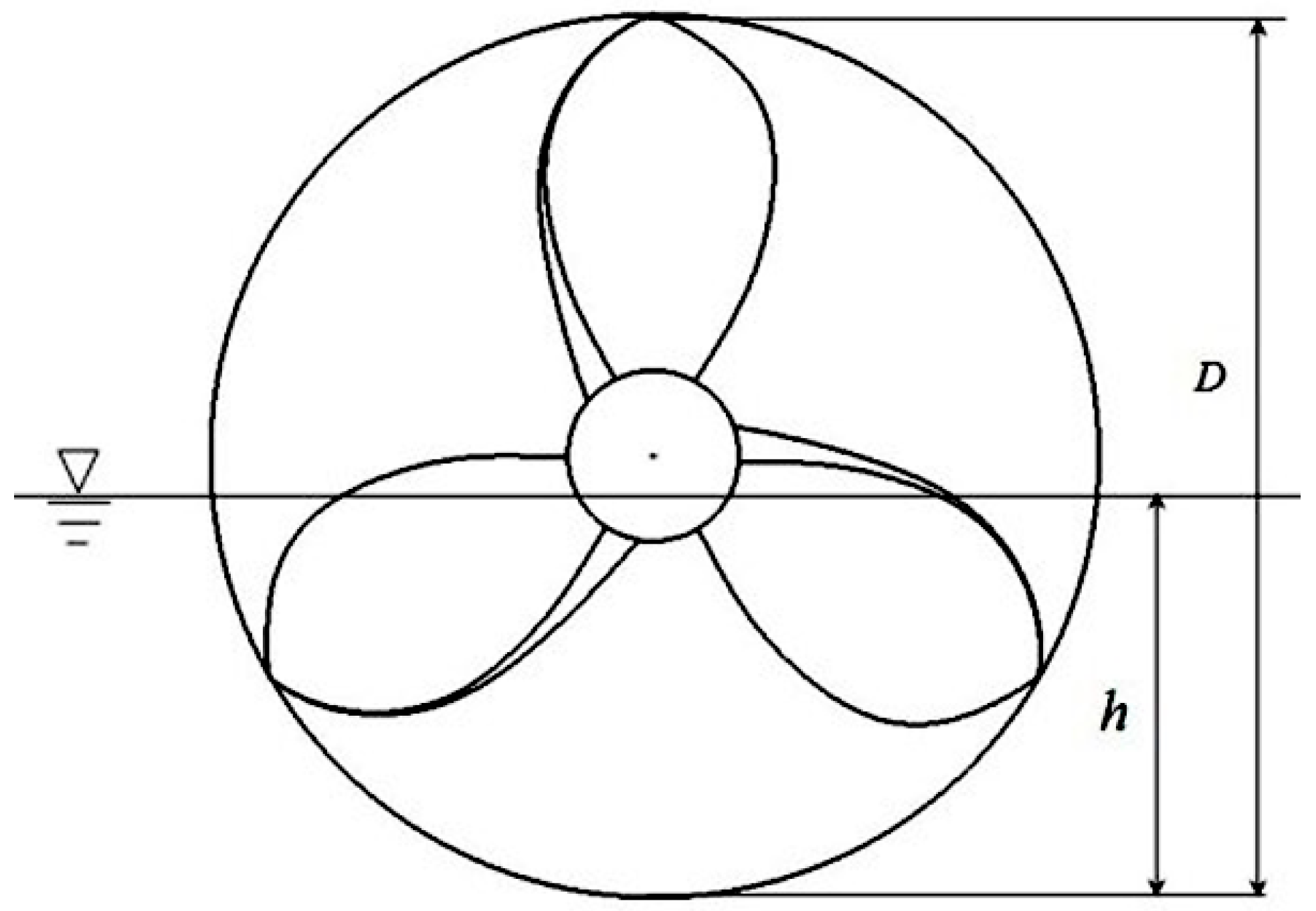
The submergence ratio of SPPs is defined as , where denotes the immersion depth of the propeller disc, is the diameter of the propeller, as shown in Figure 1.
Generally, the SPPs work on the water-air interface, and the blades rush into and out of the water in a staggered manner. In this process, the air is sucked into the water forming an air cavity, which connects the atmosphere and the paddle. This phenomenon is known as the ventilation of SPPs.
When the submergence ratio is sufficient large, the torque on the paddle will dramatically increase. For the adjustable SPPs, the torque can be reduced by decreasing the immersion depth. For the fixed SPPs, however, it is commonly difficult to adjust the immersion depth. Although the paddle may pump some air into water when it rotates, the torque can still be very large. For the purpose of torque reduction, an aeration pipe is generally installed in front of the paddle to ventilate the blades and thus reduce the torque.
2.1. SPP Model
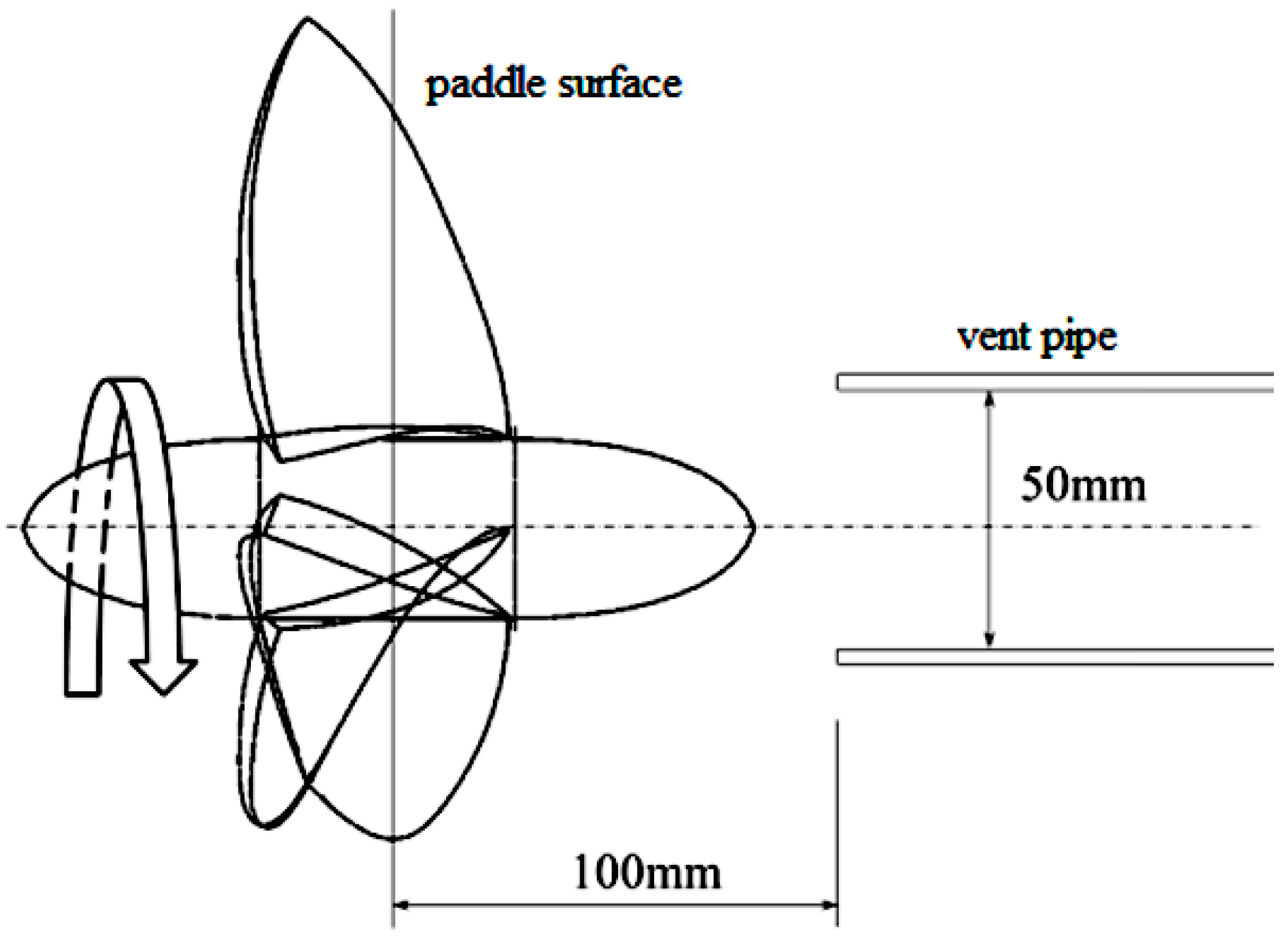
The SPP proposed for the calculation is the SPP-1 type surface-piercing propeller model given in Table 1 [6], with the rotation direction being right-handed and the profile being S-C type. The diameter of the aeration pipe is 50 mm, and the distance from the outlet of the aeration pipe to the paddle surface is 100 mm. The sketch of the propeller and the vent pipe are shown in Figure 2.
2.2. Control Equation
Under the full immersion condition, ventilation through the aeration pipe allows the paddle always being in an unsteady air-water two-phase flow field. The VOF (volume of fluid) model [13] was selected for capturing the interface between water and air. Air and water in the flow field are deemed incompressible.
Mass conservation equation can be written as:
The above equation is a general expression of the mass conservation equation, where the term Sm can be any user-defined source term added to the continuity term.
The momentum equations are given as:
where is the velocity component in the xi direction () of the Cartesian coordinate system, the fluid pressure, the fluid density, the dynamic viscosity coefficient, the time, and the volume force.
2.3. Computational Domain and Grid Division
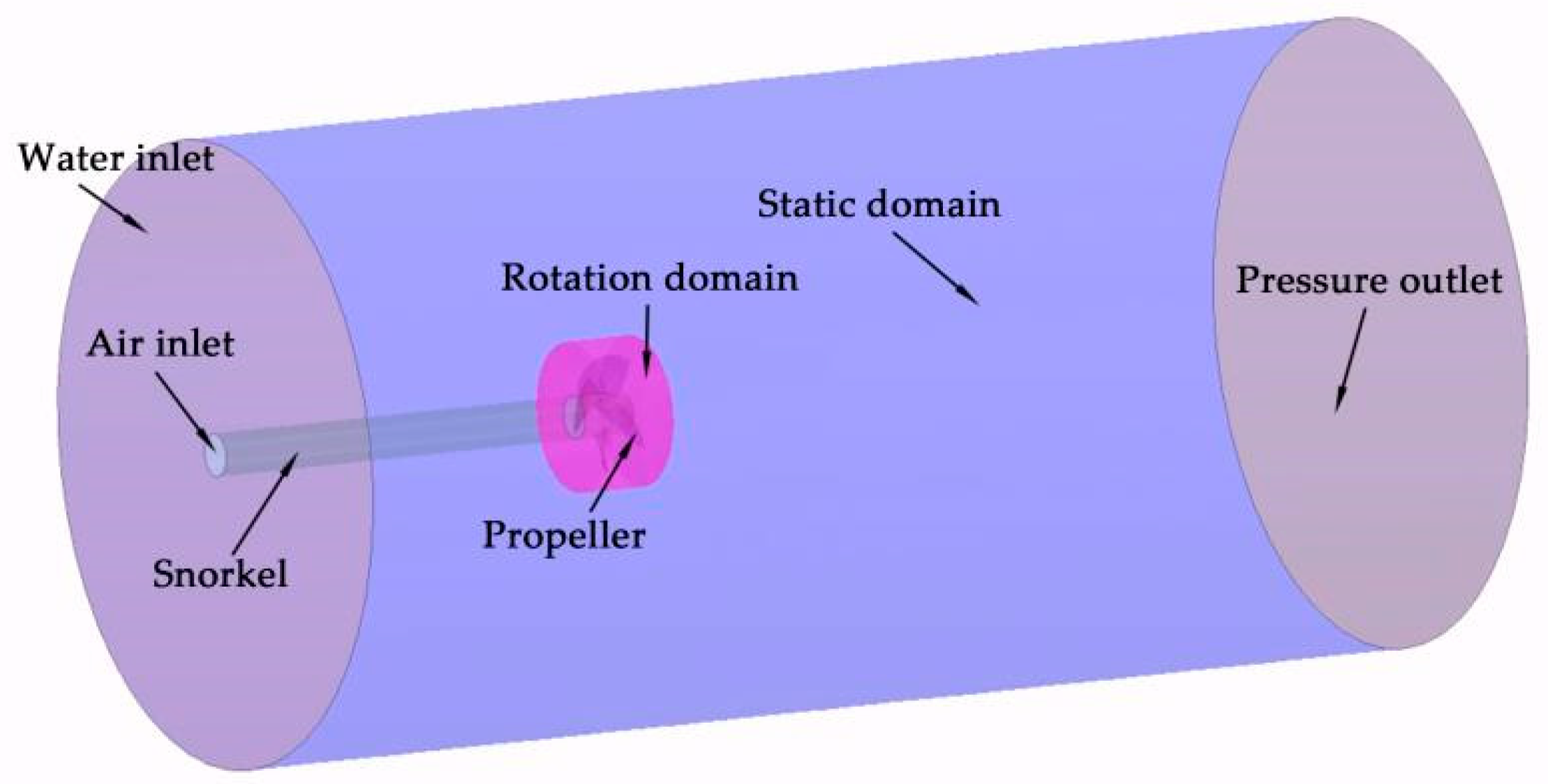
In order to make the flow field around the propeller be fully developed, and the numerical results be accurate and reliable, the size of the flow domain in the simulation should be large enough. In practice, the entire flow domain is divided into two parts: a cylindrical rotating zone containing the paddle and an outer cylindrical stationary zone. The outer diameter of the stationary zone is 5.0D, the inlet is 3.5D from the paddle plane, and the outlet is 7.0D from the paddle plane. The diameter of the rotation domain is 1.2D, and both end surfaces of the cylinder are 0.45D from the paddle surface. Figure 3 shows an oblique view of the propeller’s computational domain.
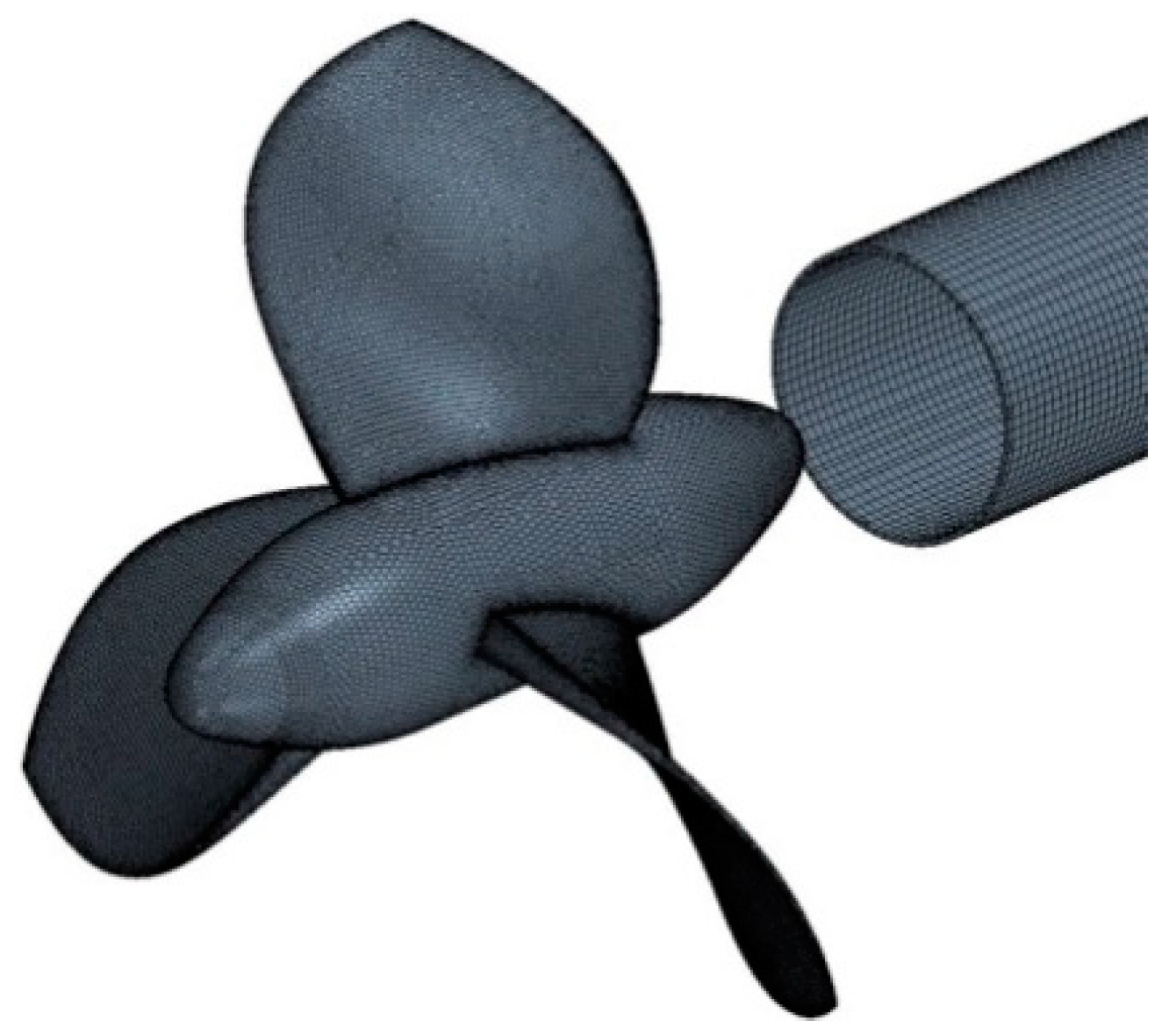
To simulate the rotation of the paddle in the flow field, the overlapped mesh method was employed. At the overlapping domain between the stationary and the rotational domains, the information of the flow field is exchanged through the overlapping grids. The mesh in the overlapping domain should be the same size as much as possible. We set the polyhedral mesh in the inner rotational domain, while the cutting body mesh in the outer stationary domain. Moreover, local mesh densification was performed around the overlapping domain. Finally, the total number of grids is 3.5 million, in which the rotation domain is 1.7 million, and the stationary domain is 1.8 million. The min and max size of computational grids are 7.65 × 10⁻⁴ mm and 11 mm, respectively. The surface mesh is shown in Figure 4.
2.4. Grid Convergence
Let Y+ be the non-dimensional wall distance defined as , where is the friction velocity at the nearest wall, the distance to the nearest wall, and the local kinematic viscosity of the fluid. In this sub-section the sensitivity of numerical results with respect to is studied. Generally, the range of dimensionless wall distance Y+ is acceptable for blade surfaces. Table 2 lists the error of the thrust coefficient and torque coefficient compared with the test value with different Y+ value. It can be seen that three errors reach minimum when the Y+ is equal to 60. Therefore, we set Y+ = 60 in the meshing setup.
Grid convergence study is important in the mesh generation process. Here four grid numbers, 1.77 million (G1), 2.5 million (G2), 3.5 million (G3), and 5 million (G4) are selected for the convergence study. The grid number and simulation results are given in Table 3. From these results, it is clearly noticed that with the growth of grid number, the results get closer to the experimental ones, i.e., the grid convergence can be guaranteed in these numbers. However, the greater the grid number, the lower computational efficiency for the numerical simulation. It is found that the accuracy was only slightly improved in the G4 case at the expense of a lot of calculation time. Hence, when determining the grid number, one should make a compromise between accuracy and efficiency. In this paper, the fine mesh of G3 was adopted in the present simulations, which achieves both computational efficiency and accuracy.
2.5. Boundary and Initial Conditions
Due to the air-suck phenomenon, the flow around the surface-piercing paddle is usually an air-water two-phase unsteady one. The density of water and air in the simulation is 997.56 kg/m3 and 1.18 kg/m3, respectively. The dynamic viscosity of water and air is 8.89 × 10⁻⁴ Pa·s and 1.86 × 10⁻⁵ Pa·s, respectively. The VOF approach was employed to track the air-water interface. The principle of this approach is to determine the interface by counting the volume ratio function of the fluid in each cell rather than the motion of the particle on the free surface.
The fluid density can be expressed as:
where is the volume fraction of the mth type of fluid in each cell, which satisfies the following condition:
In this paper, velocity inlet was divided into air velocity inlet and water velocity inlet. Both inlets have the same velocity vector. The volume fraction of the overall inlet was set as the mixture of air and water fractions, where the volume fraction of air at the air velocity inlet was set to 1, and the water volume fraction was set to 0. The outlet is set as a pressure outlet and the standard atmospheric pressure is made as the reference pressure. The outer wall of the stationary zone is set as a plane of symmetry, and the surfaces of the surface-piercing paddle and the vent pipe are set to be non-slip and non-penetrable. The outer boundary of the rotation domain is set to overlapped grids.
The second-order schemes were applied for spatial discretization and linear interpolation, as well as the time integration. The time step is 6.94 × 10⁻⁵ s, during which the propeller rotates 1° under the given rotational speed. As suggested by Blocken and Gualtieri [17], this time step makes the condition CFL 1 satisfied. The numerical calculation was performed on a PC with an Intel Xeon CPU X5690 (6 cores, 3.46 GHz), and one case simulation approximately costs 40 h.
2.6. Validation of the Numerical Setup
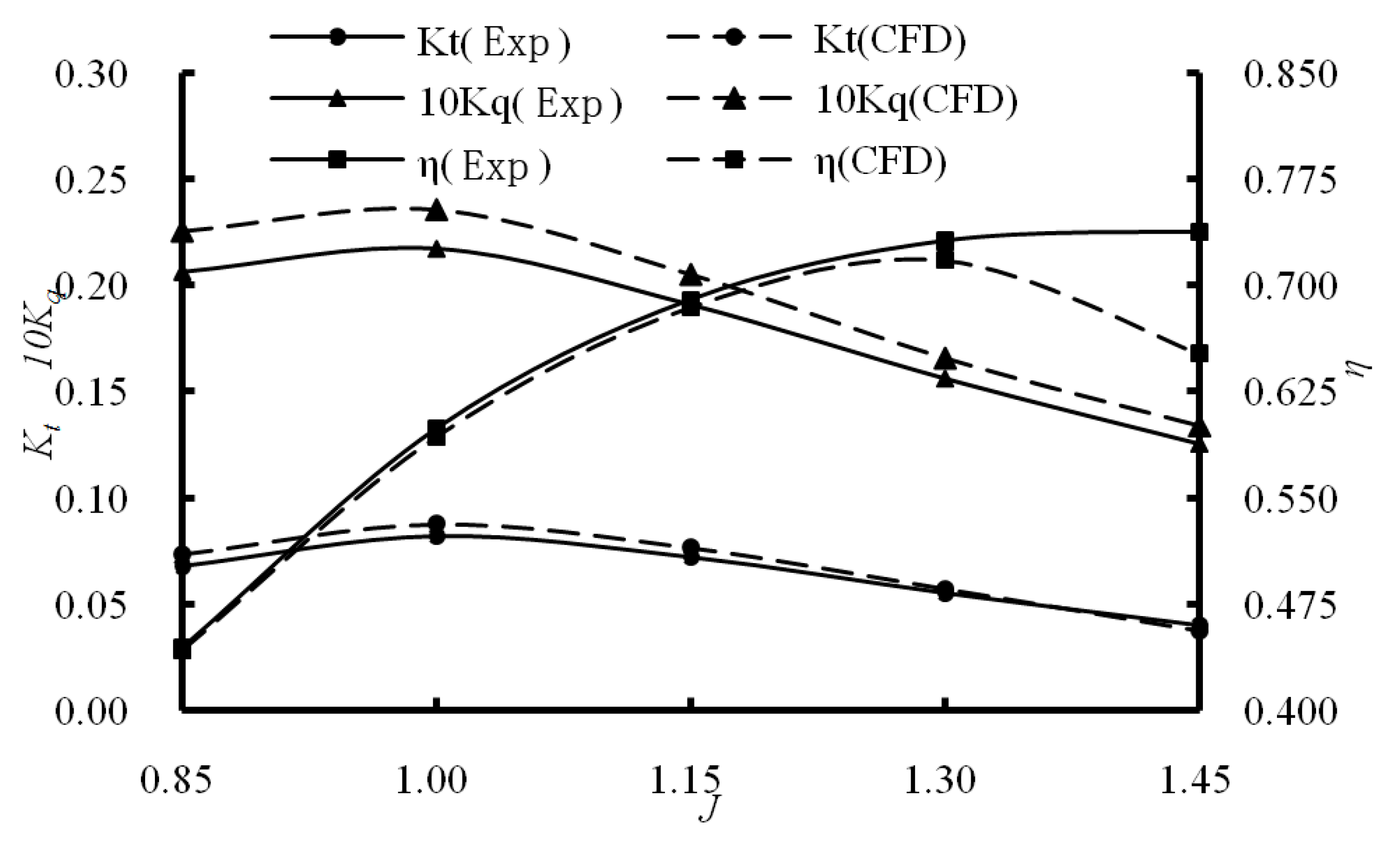
To verify the aforementioned numerical setup, the hydrodynamic performance of a propeller in the open water was investigated and compared with experimental results from Ghassemi et al. [6]. The main parameters of the SPP-1 propeller are listed in Table 1. The hydrodynamic characteristics are plotted using solid lines (see Figure 5). Let , , , and be the thrust, torque, rotational speed, and forward speed of the propeller, respectively. The relevant parameters for the propeller can be nondimensionalized as follows.
Speed coefficient:
Thrust coefficient:
Torque coefficient:
Promote efficiency:
In the numerical and experimental setup, the submergence ratio for the propeller is , and the rotational speed is n = 2400 rpm. The speed coefficient ranges from 0.85 to 1.45, which was obtained by varying the magnitude of the incoming flow velocity .
By using the CFD solver, we obtained the thrust coefficient , the torque coefficient of the propeller, and the open water efficiency . is used due to the fact that is one order smaller than and . Figure 5 compares the CFD results with the experimental ones given in Table 1 [6].
As shown in Figure 5, the thrust coefficient obtained by the CFD is slightly larger than the experimental one when , and then the discrepancy gradually decreases with the growth of . The torque coefficient has a similar trend but the discrepancy between CFD and experimental results is slightly larger than that in the case. In contrast, the open water efficiency η obtained by the CFD is always slightly smaller than the experimental one when , but the error rapidly grows with when and reaches its maximum 12% at . This study demonstrates that the numerical setup in the CFD solver is effective and can provide the required precision for the hydrodynamic simulation of the propeller with the existence of air-water interface.
3. Numerical Results of the Ventilated SPP
3.1. Calculation of Hydrodynamic Coefficient of Wigley Ship
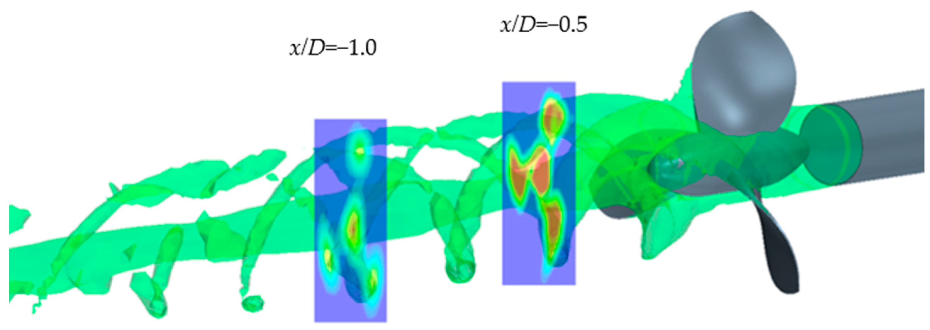
Figure 6 depicts the wake of the ventilated SPP at , from which it can be seen that the majority of the air stream flow bypasses the hub, while the rest of the flow is swung away by the rotating blades. Figure 6 displays a snapshot of the air volume fraction (green color) flowing around the rotating propeller. One can find that the trailing edges are enclosed by air bubbles due to the relatively low pressure around them. The air bubbles on the trailing edges generally stretch from the root to the tip of the blades, though on the leading edges the bubbles may only concentrate around the root domain of the blades. In the wake, three helical air bubbles are forming and rotating about the centric air stream. In the near propeller F field, the helical air bubbles and the centric air stream are connected to each other. With the flow moving downstream, the helical air bubbles gradually separate from the centric air stream, and then both helical air bubbles and centric air stream keep breaking into smaller bubbles until all of them disappear in the far field. Through setting up the interface and defining two-phase flow displayable distribution, it also shows the air and water distribution on the two cross sections and after the paddle plane. The red and blue colors refer to air and water, respectively. It can be seen that the air-content ratio gradually decreases along the downstream direction of the wake.
3.2. Effect of Ventilation on the Hydrodynamic Performance of the SPP
Table 4 compares the numerical results for the ventilated SPP with the unventilated one under full submergence condition.
From Table 4, it can be seen that the thrust coefficient and torque coefficient of the propeller decrease after ventilation. With the growth of the speed coefficient (from 0.85 to 1.30), the influence of ventilation on the thrust coefficient gradually diminishes, while the effect on the torque coefficient is reinforced. On the other hand, the efficiency of the ventilated propeller is slightly less than the unventilated one under low speed coefficient . However, with the growth of the speed coefficient , the efficiency of the ventilated propeller quickly increases as compared to the unventilated one.
As one sees, the thrust and the torque decrease after ventilation. This is mainly due to the fact that the air bubbles attached to the surfaces of the blades after ventilation. However, with the growth of the speed factor, the effect of the ventilation on the thrust coefficient is getting weaker, while the effect on the torque coefficient becomes stronger, which makes the efficiency of the ventilated propeller greater than the unventilated one.
3.3. Effect of Ventilation on the Pressure Distribution
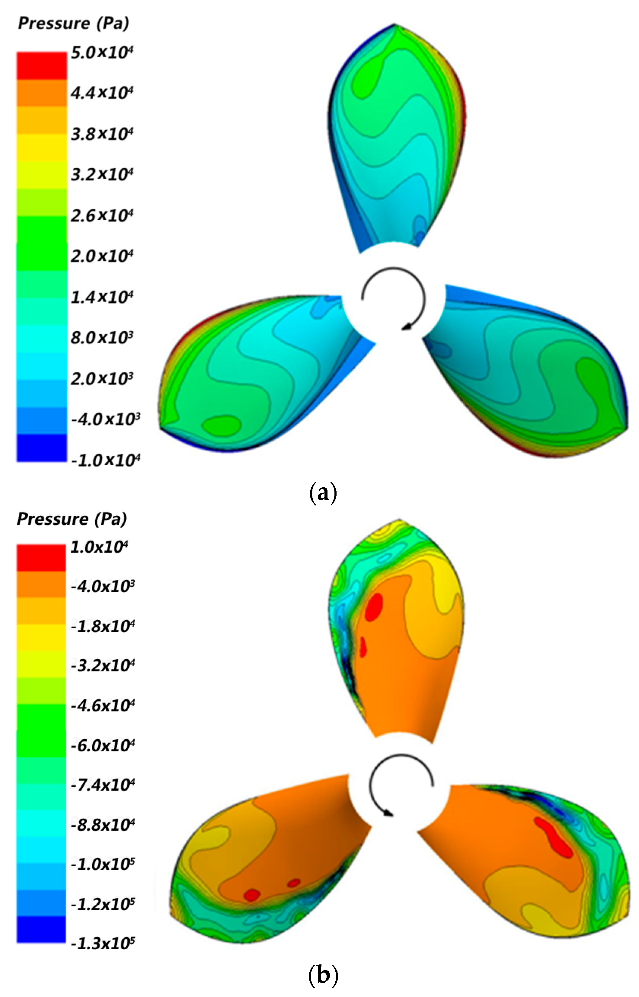
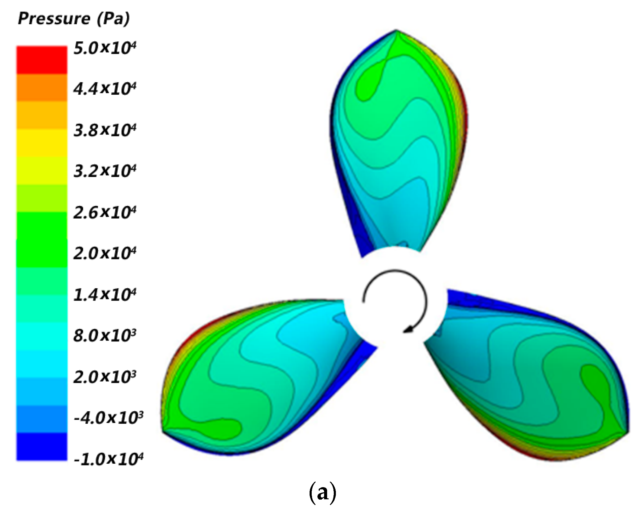
Figure 7 portrays the pressure distribution cloud on the blades of the unventilated SPP at . Figure 7a,b show the pressure distribution on the pressure surface and the suction surface, respectively. The arrows in the figures indicate the rotational direction of the propeller. From Figure 7a, one notes that on the pressure surface the high pressure is mainly concentrated on the region near the leading edge of the blades. Obviously, the closer the leading edge, the higher the pressure. While the closer the trailing edge, the lower the pressure. On the thick trailing edge, the pressure may even be negative. In contrast, as shown in Figure 7b, the lower pressure mainly locates on the region near the leading edge of the blades.
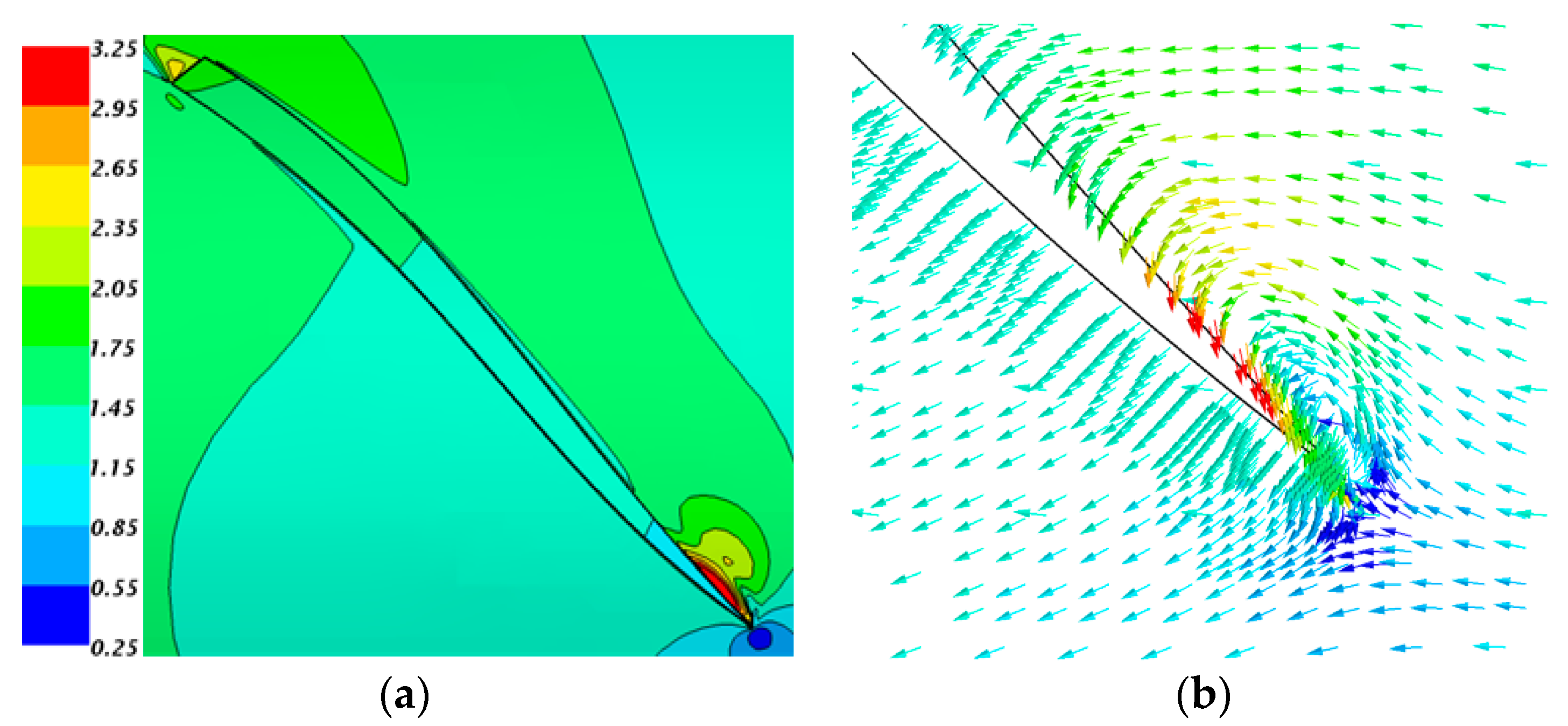
As shown in Figure 7b, there exists a pressure jump near the leading edge, which is caused by the geometric characteristics of the SPP, i.e., the relative large pitch of the SPP induces a vortex formed after the leading edge, as shown in Figure 8. Figure 8a,b depict a non-dimensional velocity distribution cloud at the 0.5R section and a non-dimensional tangential velocity vector near the leading edge, respectively. The flow velocity is nondimensionalized with respect to the forward speed of the propeller . From Figure 8a,b, one can find that there exists a high flow velocity zone on the suction surface near the leading edge. The local high velocity produces a sudden pressure drop on the suction surface. Moreover, it can be seen from Figure 8a that around the root of the thick trailing edge, the flow velocity is also very high, which makes the pressure in this zone be low and thus the air bubbles can adhere to this zone.
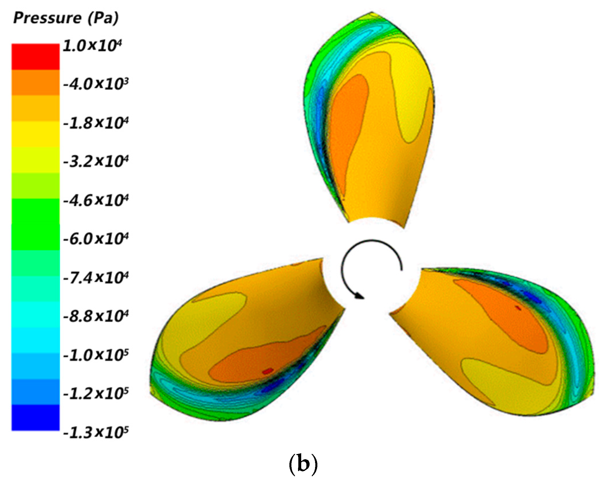
Figure 9 shows the pressure distribution on the surfaces of the ventilated SPP. Figure 9a,b are the pressure distribution on the pressure surface and the suction surface, respectively. Comparing Figure 9a with Figure 7a, it can be found that the pressure on the trailing edge of the pressure surface increases after ventilating due to the fact that air bubbles adhere to it. On the other hand, comparing Figure 9b with Figure 7b, it can be found that the area of the high pressure zone on the suction surface is significantly increased. This is because of the adsorption of air on the suction surface after ventilation. The increase in the area of the high pressure zone on the suction surface results in a reduction in the thrust and torque of the SPP.
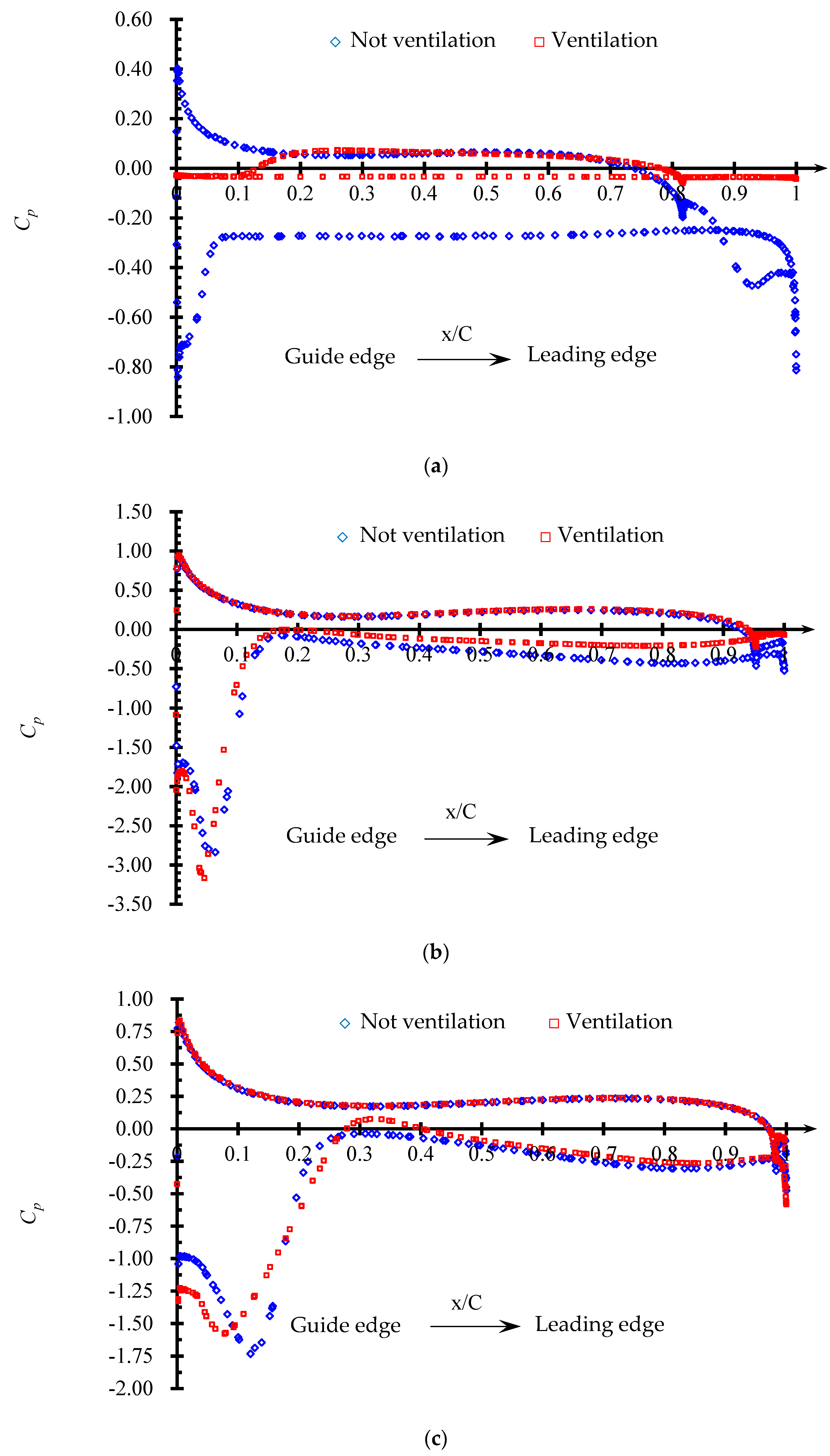
Figure 10 plots the pressure distribution at on various profiles (0.24R, 0.50R and 0.70R) of the ventilated/unventilated SPP. is the pressure coefficient. Blue and red lines refer to the pressure distribution profiles of the unventilated and ventilated SPP, respectively. From Figure 10a one can see that on the profile near the root (0.24R), when there is no ventilation, the difference between the pressure on the pressure surface and the one on the suction surface is very large, especially near the leading edge. After ventilating, the pressure on the suction surface of the blade significantly increases and evenly distributes along the entire chord direction. The pressure almost remains unchanged because the air bubbles completely cover the root region of the blades, and in the vicinity of the leading edge (), the pressure on the pressure surface and the suction surface are almost the same. This is because both the pressure surface and suction surface near the leading edge are covered by the air bubble. The same phenomenon can be observed around the trailing edge.
As shown in Figure 10b, on the profile 0.50R, the pressures on the pressure surface of the ventilated and unventilated SPP are almost the same. And only on the suction surface the pressure from the ventilated SPP is slightly bigger than the unventilated one due to the ventilation.
On the profile closer to the tip of the blade (0.70R), see Figure 10c, the pressure distribution on the pressure surface of the ventilated and unventilated SPP are completely the same. Only in the vicinity of the guide edge were the pressures on the suction surface of the ventilated and unventilated SPP slightly different, which is due to the non-uniformity of the flow field.
Comparing Figure 10a–c, one observes that the effect of ventilation on the pressure distribution of the SPP is limited to a zone in the vicinity of the blade root. In this zone, the ventilation has significant effect on the pressure. And along the outward radius direction, the effect of the ventilation gradually diminishes.
4. Conclusions
In this paper, the effect of artificial ventilation on the hydrodynamic performance of a surface-piercing propeller (SPP) was investigated using the CFD technique. The present work is different from previous works as follows. In previous works, such as Ghassemi et al. [6,7], Young et al. [9,10,11], and Alimirzazadeh et al. [13], the SPPs work under half immersed conditions with the propeller naturally ventilated. In such conditions, all blades experience periodic water-entry and water-exit processes. While in the present work, the SPP works under full immersion conditions with artificial ventilation through a vent pipe in front of the propeller disc. In such condition, all blades are partially surrounded by air bubbles, in which the phenomenon as well as the hydrodynamic performance of the SPP are significantly different from those given in literatures. The main conclusions are summarized as follows:
- (1)
- The turbulence model SST and the overlapped mesh method can make faithful simulation for the ventilated SPP in unsteady flow field, and precisely forecast its hydrodynamic performance.
- (2)
- In the wake of the ventilated SPP, there are three helical air bubbles that rotate about the centric air stream. With the flow moving downstream, the helical air bubbles and the centric air stream gradually break into smaller bubbles until all of them disappear in the far field.
- (3)
- The effect of ventilation on the pressure distribution of the SPP is limited to a zone in the vicinity of the blade root (less than 0.5R). In this zone, the ventilation has significant effect on the pressure, and along the outward radius direction, the effect gradually diminishes.
- (4)
- The thrust coefficient () and torque coefficient () of the propeller decrease after ventilation. However, with the growth of the forward speed of the SPP, the influence of the ventilation on the thrust coefficient is smaller than on the torque coefficient, which makes the efficiency () of the ventilated SPP, be significantly greater than that of unventilated SPP. The numerical results demonstrate the effectiveness of the ventilation approach for improving the hydrodynamic performance of the SPPs for high speed planning crafts.
Author Contributions
D.Y. performed the numerical calculations; Z.R. and Z.G. (Zhiqun Guo) completed the geometric modeling and mesh generation; Z.G. (Zhiqun Guo) and Z.G. (Zeyang Gao) analyzed the post-processing data; D.Y. wrote the paper.
Funding
This project is supported by the National Natural Science Foundation of China (Grant No. 51509053, No. 51579056, and No. 51579051).
Conflicts of Interest
The authors declare no conflict of interest. The founding sponsors had no role in the design of the study; in the collection, analyses, or interpretation of data; in the writing of the manuscript, and in the decision to publish the results.
References
- Ding, E.B.; Tang, D.H.; Zhou, W.X. A review of research on semi-submerged propellers. J. Ship Mech. 2002, 6, 75–84. [Google Scholar]
- Zhao, R.; Faltinsen, O. Water entry of two-dimensional bodies. J. Fluid Mech. 1993, 246, 593–612. [Google Scholar] [CrossRef]
- Young, Y.L.; Savander, B.R. Numerical analysis of large-scale surface-piercing propellers. Ocean Eng. 2011, 38, 1368–1381. [Google Scholar] [CrossRef]
- Yari, E.; Ghassemi, H. Numerical analysis of surface piercing propeller in unsteady conditions and cupped effect on ventilation pattern of blade cross-section. J. Mar. Sci. Technol. 2016, 21, 501–516. [Google Scholar] [CrossRef]
- Yu, Y.Q.; Yu, J.X.; Ding, E.B. Numerical study of two-dimensional “cup” shaped supercavitation cross-section inflow. J. Ship Mech. 2008, 12, 539–544. [Google Scholar]
- Ghassemi, H.; Shademani, R. Hydrodynamic characteristics of the surface-piercing propellers for the planing craft. J. Mar. Sci. 2009, 8, 267–274. [Google Scholar]
- Kinnas, S.A.; Young, Y.L. Modeling of cavitating or ventilated flows using BEM. Int. J. Numer. Methods Heat Fluid Flow 2003, 13, 672–697. [Google Scholar] [CrossRef]
- Young, Y.L.; Kinnas, S.A. Numerical analysis of surface piercing Propellers. In 2003 Propeller and Shaft Symposium; Society of Naval Architects and Marine Engineers: Virginia Beach, VA, USA, 2003. [Google Scholar]
- Young, Y.L.; Kinnas, S.A. Analysis of supercavitating and surface piercing propeller flows via BEM. J. Comput. Mech. 2003, 32, 269–280. [Google Scholar] [CrossRef]
- Shi, Y.X.; Zhang, L.X.; Shao, X.M. Numerical simulation of hydrodynamic performance of semi-submerged propeller. Mechatron. Eng. 2014, 31, 985–990. [Google Scholar]
- Alimirzazadeh, S.; Roshan, S.Z.; Seif, M.S. Unsteady RANS simulation of a surface piercing propeller in oblique flow. Appl. Ocean Res. 2016, 56, 79–91. [Google Scholar] [CrossRef]
- CD-adapco Group. STAR-CCM+ User Guide Version 9.06; CD-adapco Group: Melville, NY, USA, 2014. [Google Scholar]
- Zhang, J.; Fang, J.; Fan, B.Q. A review of theories and applications of VOF methods. Adv. Sci. Technol. Water Resour. 2005, 4, 67–70. [Google Scholar]
- Menter, F.R. Zonal two-equation k-ω turbulence model for aerodynamics flows. In Proceedings of the 23rd Fluid Dynamics, Plasmadynamics, and Lasers Conference, Orlando, FL, USA, 6–9 July 1993; AIAA Paper 93-2906. The American Institute of Aeronautics and Astronautics (AIAA): Reston, VA, USA, 1993. [Google Scholar]
- Calomino, F.; Alfonsi, G.; Gaudio, R.; D’lppplito, A.; Lauria, A.; Tafarojnoruz, A.; Artese, S. Experimental and Numerical Study of Free-Surface Flows in a Corrugated Pipe. Water 2018, 10, 638. [Google Scholar] [CrossRef]
- Huang, S.; Wang, C.; Wang, S.Y. Application and comparison of different turbulence models in the calculation of propeller hydrodynamic performance. J. Harbin Eng. Univ. 2009, 5, 481–485. [Google Scholar]
- Blocken, B.; Gualtieri, C. Ten iterative steps for model development and evaluation applied to Computational Fluid Dynamics for Environmental Fluid Mechanics. Environ. Model. Softw. 2012, 33, 1–22. [Google Scholar] [CrossRef]
Figure 1.
The submergence ratio of surface-piercing propellers (SPPs), which is defined as the ratio of the immersion depth to the propeller diameter .
Figure 1.
The submergence ratio of surface-piercing propellers (SPPs), which is defined as the ratio of the immersion depth to the propeller diameter .

Figure 2.
The sketch of the propeller and the vent pipe.

Figure 3.
Oblique view of propeller and computational field.

Figure 4.
Mesh on the propeller and aeration pipe.

Figure 5.
Comparison of CFD and experimental results at

Figure 6.
The wake after the ventilated propeller at when (left section) and (right section).

Figure 7.
The pressure distribution on the blades at under unventilated condition. (a) The pressure distribution on the pressure surface; (b) The pressure distribution on the suction surface.
Figure 7.
The pressure distribution on the blades at under unventilated condition. (a) The pressure distribution on the pressure surface; (b) The pressure distribution on the suction surface.

Figure 8.
Non-dimensional velocity distribution cloud at 0.5R section. (a) The non-dimensional velocity cloud; (b) The non-dimensional velocity vector cloud near the leading edge.
Figure 8.
Non-dimensional velocity distribution cloud at 0.5R section. (a) The non-dimensional velocity cloud; (b) The non-dimensional velocity vector cloud near the leading edge.

Figure 9.
The pressure distribution on the blades at under ventilated condition. (a) The pressure distribution on the pressure surface; (b) The pressure distribution on the suction surface.
Figure 9.
The pressure distribution on the blades at under ventilated condition. (a) The pressure distribution on the pressure surface; (b) The pressure distribution on the suction surface.


Figure 10.
The pressure distribution profiles at . (a) The pressure distribution profile at 0.24R; (b) The pressure distribution profile at 0.50R; (c) The pressure distribution profile at 0.70R.
Figure 10.
The pressure distribution profiles at . (a) The pressure distribution profile at 0.24R; (b) The pressure distribution profile at 0.50R; (c) The pressure distribution profile at 0.70R.


Table 1.
SPP-1 propeller geometric parameters [6].
Table 1.
SPP-1 propeller geometric parameters [6].
| Parameters | |
|---|---|
| Diameter D | 0.2 |
| Tilt angle/° | 10 |
| Number of leaves Z | 3 |
| Pitch ratio P/D | 1.6 |
| Disk ratio AE/AO | 0.5 |
| Hub diameter ratio d/D | 0.2 |
| Side angle/° | 0 |
| Profile | S-C |
Table 2.
Results for the Y+ for selection.
| Y+ | ||||
|---|---|---|---|---|
| Exp. | 0.3093 | 0.8579 | ||
| 30 | 0.2759 | 0.7758 | −10.81% | −9.57% |
| 40 | 0.2791 | 0.7840 | −9.77% | −8.61% |
| 50 | 0.2825 | 0.7956 | −8.69% | −7.26% |
| 60 | 0.2857 | 0.8016 | −7.65% | −6.56% |
| 70 | 0.2836 | 0.7977 | −8.33% | −7.01% |
| 80 | 0.2800 | 0.7843 | −9.48% | −8.57% |
| 90 | 0.2786 | 0.7779 | −9.95% | −9.32% |
Table 3.
Results from the grid convergence.
| Grid | Control Volumes | ||||
|---|---|---|---|---|---|
| G1 | 1,770,000 | 0.2756 | 10.89% | 0.7761 | 9.53% |
| G2 | 2,500,000 | 0.2806 | 9.28% | 0.7874 | 8.21% |
| G3 | 3,500,000 | 0.2857 | 7.63% | 0.8016 | 6.65% |
| G4 | 5,000,000 | 0.2884 | 6.77% | 0.8070 | 5.93% |
Table 4.
Numerical results for the SPP under full submergence conditions.
| Speed Coefficient | Unventilated SPP | Ventilated SPP | |||||
|---|---|---|---|---|---|---|---|
| 0.85 | Value | 0.3763 | 0.9679 | 0.5259 | 0.3199 | 0.8452 | 0.5120 |
| Variation/% | −14.99 | −12.68 | −2.64 | ||||
| 1.00 | Value | 0.3093 | 0.8579 | 0.5738 | 0.2749 | 0.7441 | 0.5880 |
| Variation/% | −11.12 | −13.26 | 2.47 | ||||
| 1.15 | Value | 0.2495 | 0.7502 | 0.6087 | 0.2308 | 0.6462 | 0.6537 |
| Variation/% | −7.49 | −13.86 | 7.39 | ||||
| 1.30 | Value | 0.1897 | 0.6426 | 0.6108 | 0.1867 | 0.5389 | 0.7168 |
| Variation/% | −1.58 | −16.14 | 17.35 | ||||
© 2018 by the authors. Licensee MDPI, Basel, Switzerland. This article is an open access article distributed under the terms and conditions of the Creative Commons Attribution (CC BY) license (http://creativecommons.org/licenses/by/4.0/).
Share and Cite
MDPI and ACS Style
Yang, D.; Ren, Z.; Guo, Z.; Gao, Z. Numerical Analysis on the Hydrodynamic Performance of an Artificially Ventilated Surface-Piercing Propeller. Water 2018, 10, 1499. https://doi.org/10.3390/w10111499
AMA Style
Yang D, Ren Z, Guo Z, Gao Z. Numerical Analysis on the Hydrodynamic Performance of an Artificially Ventilated Surface-Piercing Propeller. Water. 2018; 10(11):1499. https://doi.org/10.3390/w10111499
Chicago/Turabian StyleYang, Dongmei, Zhen Ren, Zhiqun Guo, and Zeyang Gao. 2018. "Numerical Analysis on the Hydrodynamic Performance of an Artificially Ventilated Surface-Piercing Propeller" Water 10, no. 11: 1499. https://doi.org/10.3390/w10111499
Note that from the first issue of 2016, this journal uses article numbers instead of page numbers. See further details here.