“E = mc²” of Environmental Flows: A Conceptual Framework for Establishing a Fish-Biological Foundation for a Regionally Applicable Environmental Low-Flow Formula

Abstract

Determination of environmental flows at the regional scale has been complicated by the fine-scale variability of the needs of aquatic organisms. Therefore, most regional methods are based on observation of hydrological patterns and lack evidence of connection to biological responses. In contrast, biologically sound methods are too detailed and resource-consuming for applications on larger scales. The purpose of this pilot project was to develop an approach that would breach this gap and provide biologically sound rules for environmental flow (eflow) estimation for the region of Poland. The concept was developed using seven river sites, which represent the four of six fish-ecological freshwater body types common in Poland. Each of these types was distinguished based on a specific fish community structure, composed of habitat-use guilds. The environmental significance of the flows for these communities was established with help of the habitat simulation model MesoHABSIM computed for each of the seven sites. The established seasonal environmental flow thresholds were standardized to the watershed area and assigned to the corresponding water body type. With these obtained environmental flow coefficients, a standard-setting formula was created, which is compatible with existing standard-setting approaches while maintaining biological significance. The proposed approach is a first attempt to use habitat suitability models to justify a desktop formula for the regional scale eflow criteria.

1. Introduction

In Europe, continent-wide investigations of ecological status and human-induced pressures have documented that about half of the European bodies of water hold less than ideal ecological status or potential. Hydromorphological changes are the most widespread pressure on the ecological status of European Union (EU) water bodies [1].

One key source of hydromorphological change is excessive water withdrawal, dramatically reducing habitat availability for aquatic animals [2,3,4]. A recognized mitigation and management option for that is the introduction and establishment of an environmental flow (eflow) requirement, which will secure the needs of aquatic and riparian communities [5,6,7].

The Environmental Flow Guidance document [8] defines eflows as a “hydrological regime consistent with the achievement of the environmental objectives of the WFD,” such as:

• Non-deterioration of the existing ecological status,
• Achievement of good ecological status in a natural surface water body, and
• Compliance with standards and objectives for protected areas.

In order to determine eflows, we need to investigate the impact of flow manipulation on aquatic and semi-aquatic organisms and identify threshold flow levels, which assure that sustainable populations are maintained. These thresholds can serve in a regulatory process as benchmarks for allowing the use of water from rivers and streams or for triggering mitigation actions [9].

The structure and functioning of aquatic ecosystems are largely dependent on various types of flows (low flows, high flows, flow pulses, etc.). Extreme phenomena, such as floods and droughts, play the role of an environmental features regulators and change the structure of the population by selective elimination of species [10]. Low flows control water chemistry, dry low areas in floodplains, limit the usable area of the habitat and are often associated with a higher water temperature and lower oxygen solubility. On the other hand, low flows provide conditions for the development of larval stages and juvenile fish, creating shallow coastal zones: warm, rich in food, and protects against water predators. Maintenance flows (i.e., high flows) play a key role in the structure and functioning of the aquatic ecosystem. Short-term changes in the flow caused by freshets can provide aquatic organisms with the necessary rest from stressful low-flow conditions. Small floods provide active access to fish and other organisms to floodplains and habitats, such as side canals, backwaters, and wetlands. Large floods can carry significant amounts of sludge, wood, and stone as well as organic matter, creating new habitats and refreshing water quality conditions in both mainstream and floodplains. In general, we can distinguish two major types of eflow thresholds that describe low flow and maintenance flow requirements. Low-flow thresholds require detailed, quantitative determination, while maintenance flow thresholds can be handled in a more qualitative way. This is because for low-flow thresholds, the overall small quantity of water in a river requires higher precision, but also because during drought conditions, the anthropogenic water demands (and therefore the water value) are greater altogether. For the maintenance flows (i.e., high flows) coarser quantities as well as frequency and duration influence the biota [11,12].

From a management perspective, eflow guidelines need to be easy to define and inexpensive to apply over whole regions [13,14]. From an environmental resource protection perspective, they should be sufficiently detailed for capturing biological response to environmental change [15].

Setting regional standards for environmental flows to protect riverine ecosystems has been a goal of resource managers since the early 19th century. Hundreds of methods were developed towards this goal (see Reference [16]); however, they are not necessarily similar or compatible with each other. Nowadays, these methods can be grouped into four major classes: standard settings, desktop hydrological methods, holistic approaches, and physical habitat model-based techniques. The complexity and accuracy of the methods increases, from former to latter, while their applicability at the regional scale declines [8].

Out of the many methods used worldwide, only habitat models are capable of capturing the detail necessary to establish a biological foundation for environmental low flows. For most, however, they are applied in site-specific context and lack procedures allowing the transfer of information to the macroscale. The majority of standard settings and hydrological methods are easy to apply in a regional context, but do not have the appropriate biological underpinning that would justify the choice of low-flow threshold levels.

One solution proposed in the Environmental Flow Guidance [8] is to use different types of methods for different scales of assessment, i.e., hydrological and holistic at the regional level, and habitat on the site-specific level. This, however, does not resolve the issue associated with biological representativeness of low eflows, as discussed before.

Therefore, the purpose of this study was to close this gap and provide a sound biological basis for the determination of low eflow thresholds that would be applicable at the regional scale. The novelty of the approach is the application of fish habitat simulation models as a foundation for a regional rule setting, by establishing extrapolation framework, which utilizes biological, geomorphic, and hydrologic upscaling approaches. The concept has been developed as a part of an investigation defining the eflow methods to be applied in all of Poland as a foundation for future water management legislation.

In 2014, the Polish National Water Management Authority contracted a study for the development of an eflow methodology, which could be adopted in the year 2020 to assure conformity with the Water Framework Directive. The updated method is intended to replace the currently used standard-setting methodology according to Kostrzewa, which was developed in early 1970 [17]. The Kostrzewa method prescribed “untouchable” flows as a product of mean annual low flow and a regionally specific coefficient estimated from analysis of a long-term flow time series of 85 gauges in Poland. Although more standard-setting methods have been developed since, with some modifications, the original is still applied country-wide. Most commonly, one low-flow value for the entire year is prescribed in water use permits. It was preferable to the agency to create a more biologically sound policy, which should fit well into the current administrative procedures.

This proof of concept project was designed to dedicate the first two years to the development of a conceptual framework and its application at seven pilot study sites selected across the country. Four approaches were used as a foundation for this purpose: the Kostrzewa method, the Target Fish Community approach, MesoHABSIM, and a Multiscale Hierarchical Framework [18,19,20,21]. The general scheme of methodological approach leading to the determination of the eflow calculation formula is presented in Figure 1.

2. Materials and Methods

Table 1. List of acronyms used.

Acronym	Explanation
A	Watershed Area
CA	Channel Area
CHSC	Conditional Habitat Suitability Criteria
FET	Fish Ecological Type
HMU	Hydromorphological Unit
HST	Habitat Stressor Tresholds
HUG	Habitat-Use Guilds
HYMO	Hydromorphology
MesoHABSIM	Mesohabitat Simulation Model
NHC	Multiscale Hierarchical Framework
MSHF	Non-Hierarchical Cluster
P	Eflow Coefficient
Q	Specific Flow in l·m2·s−1
RWB	Representative Water Body
TFC	Target Fish Community
UCUT	Uniform Continuous Under Threshold

defines all acronyms used in this work.

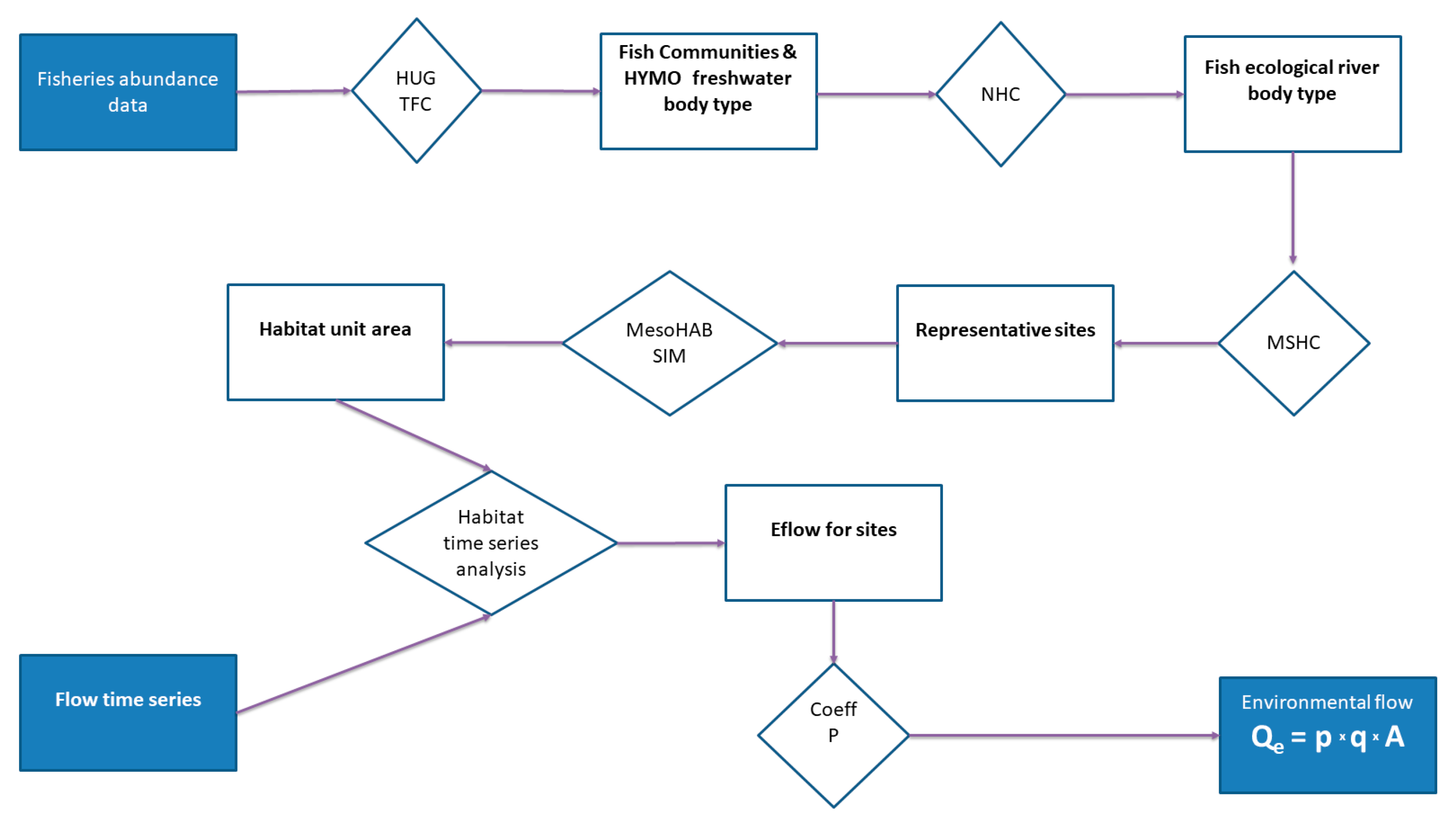
2.1. The Concept of the Extrapolation Framework

Since it was necessary to apply site-specific studies to determine flow influence on aquatic organisms, we created a framework that allowed for scientifically sound extrapolation of obtained results to the scale of the entire country. The foundation of this concept was a classification of water bodies according to expected fish communities, derived from rich, national fishery monitoring data. Implementing the Water Framework Directive, running waters across the entire European Union were divided into approximately homogenous water bodies [22]. In Poland, the classification included 4322 of such water bodies, which were grouped into 26 geomorphic types [23]. Fish samples were taken across the country, using a standardized methodology to assess ecological status [24,25]. The distribution of the sampling sites did not specifically target geomorphic types, but rather broader spatial dispersal of the samples across the country. Hence, it could not be expected that species distribution would reflect the quantitative distribution of geomorphic water body types. Still, most of the common geomorphic types were represented by at least one sample. In Poland, over 1000 sites were sampled between 2008 and 2014, of which 409 were assessed as having only limited anthropogenic pressure (pressure class 1–3) and were chosen for classification purposes.

To provide the appropriate level of generalization, rearing life stages of native fish species in Poland were grouped into habitat-use guilds [26,27]. The participation in the guilds was defined based on literature surveys and the results of expert workshops. The quantitative distribution of these guilds in 409 electrofishing samples, in association with geomorphic river types as covariate, was analyzed with non-hierarchical cluster analysis. This allowed us to group the waterbodies into fish ecological types (FET), distinguished by specific target fish communities [18]. Since the number of samples was over 200 and the clustering for large applications (CLARA) algorithm presented higher stability in cross validation, it was used for the clustering [28]. The CLARA method extends the k-method approach for a large number of objects. The number of clusters was determined with the help of scree plots of average within-cluster dissimilarities and average silhouette widths [29]. Cluster stability was assessed using the Clusterwise Jaccard bootstrap mean, as suggested by Hennig [30]. Eventually, the significance of selected clusters was verified with the help of analysis of group similarities (ANOSIM). As a tool, we used R library packages cluster and vegan [31]. Target fish communities were calculated for each cluster. Eventually, six identified clusters were ordered and numbered, according to the declining proportion of rheophylic species.

In the process of developing a method to identify environmental flow needs for these template communities, we investigated representative water bodies (RWBs). The selection of segments and appropriate representative sites was accomplished by building upon a Multiscale Hierarchical Framework [19]. This multi-scale approach to investigate hydromorphology focused on geomorphological characteristics that influenced the character and dynamics of river channels, as well as their floodplains across space. It involves delineation of spatial units at different scales (biogeographic region, catchment, landscape unit, and river reach), using Geographic Information System (GIS) tools and algorithms analyzing remote sensing datasets and geographical databases. Each unit was characterized according to a range of parameters presented in

Table 2. List of characteristics extracted at different spatial scales.

Spatial Scale	Category	Characteristic Type	Quantifiable Characteristics
Catchment and landscape units		Size, morphology	Catchment area; WFD size category; max., average, min. Elevation; WFD elevation zones
		Geology	Rock type classes
		Land cover	Proportion under land cover classes
Reach	Channel dimensions (planform, gradient)		Average gradients
			Sinuosity index
			Braiding index
			Anabranching index
	Physical pressures	River bed conditions	Number of channels blocking structures
		River bank condition and lateral continuity	Bank reinforcement
			Embankments
			Channel-crossing/blocking structures
		Riparian corridor connectivity	Floodplain accessible by flood water
			Spanning structures

.

Hence, the selection process involved the following steps. First, seven watersheds considered to be of low impact were proposed for investigation by the Regional Water Authorities. An analysis of the GIS data at the watershed and landscape unit scales followed to verify these expectations. One more watershed (River Mienia) was added in this process by the study team. Second, geomorphologically homogenous segments were identified in each of the watersheds. The final stage focused on selection of the least altered (reference) river segment in each catchment, selecting units with the lowest number of physical pressures and the most natural vegetation structure. A representative site was chosen for each segment, such that it would capture the variety of geomorphic features, assuming a minimum length exceeding 80 times the average river width. Eventually each site was assigned an appropriate FET and consequently a target community structure (Figure 2).

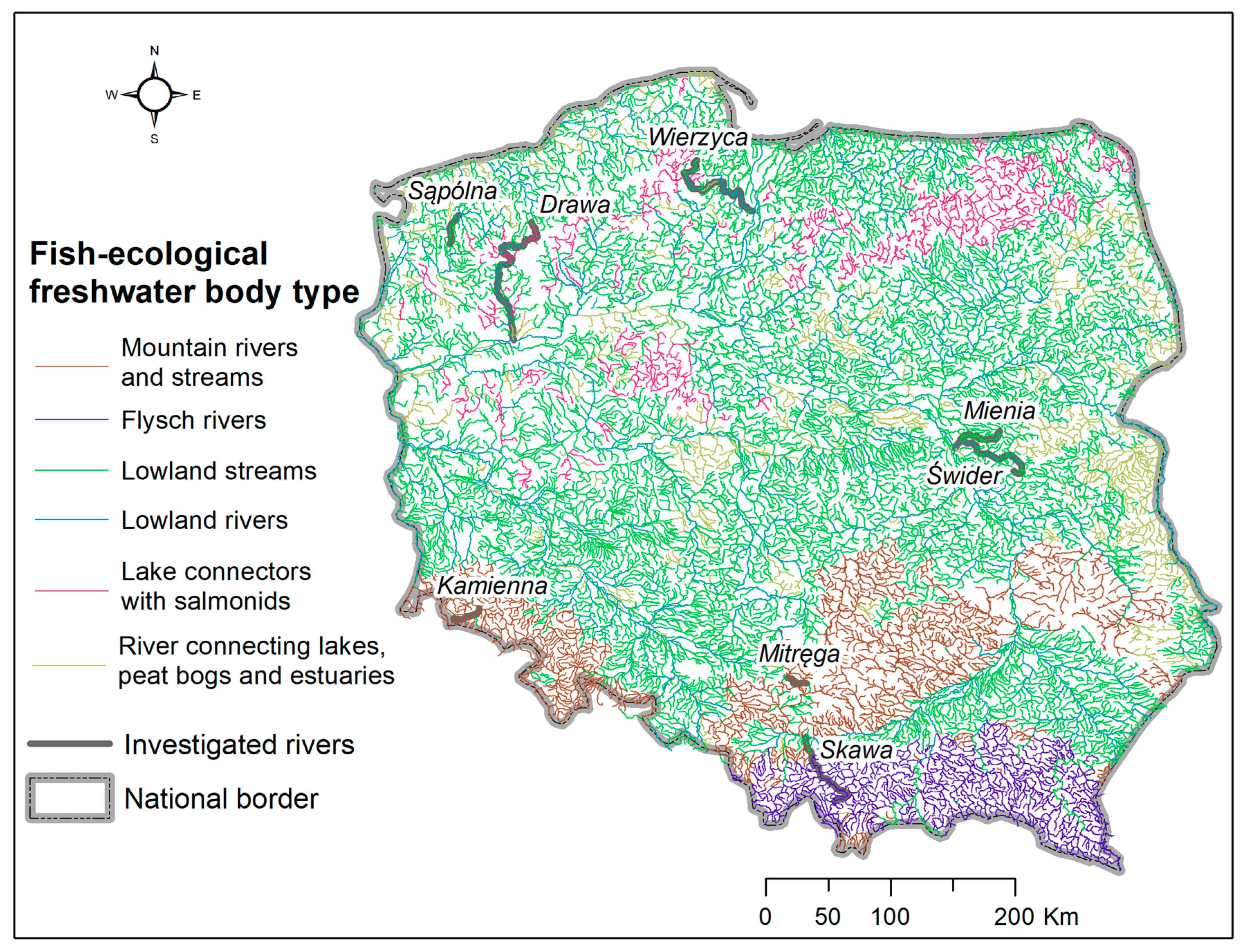
2.2. Data Collection and Analysis

In spring and summer 2015, each of selected representative sites (Figure 2) was sampled at three to four flows within the range between medium and annual low flow. The sampling was conducted using the standard MesoHABSIM methodology [21]. Hydromorphological units (HMU) were annotated using handheld computers and flow meters on aerial imagery obtained by low flying drones. The data was processed on a GIS platform, in order to produce hydromorphological maps. The habitat model for fish guilds and community structures was calculated with the help of SIM-Stream 8.0 software [32].

To provide eflow criteria representing the needs of different life stages, the year was divided into three or four bioperiods: rearing and growth (July–September/October), fall spawning (rivers with salmonid presence only) (October–November), overwintering (November/December–February), and spring spawning (March–June). For each bioperiod, a habitat-use guild, based on the fish community structure, was established. In summer, species were grouped into rearing habitat-use guilds, and for spring and fall, into spawning habitat-use guilds (Appendix A,

Table A1. Habitat-use guilds defined for river fauna in Poland, together with habitat-use criteria defined for each guild. The criteria highlighted in bold are critical, i.e., need to be fulfilled for habitat to be suitable. The substrate types (choriotope) are according to Austrian Norm (ON 6232).

#	Guild	Species	Water Depth (m)	Water Velocity (ms−1)	Choriotop Type	HMU Type	Cover
Rearing guilds—fish species grouped according to feeding and shelter habitats
1	Highly rheophilic	Salmo salar	0.25–1.5	0.3–1.2	mega-, makro-, meso-, mikro-lithal	riffle, ruffle, cascade, reef, fast run, run, pool	boulders, undercut banks, woody debris
		Salmo trutta fario
		Salmo trutta trutta
		Hucho hucho
		Cottus gobio
		Cottus poecilopus
2	Rheophilic—gravel bottom	Barbus barbus	0.3–2.0	0.15–0.90	makro-, meso-, mikro-lithal, psammal	riffle, ruffle, cascade, fast run	boulders
		Barbus peloponnesius
		Barbus cyclolepis
		Vimba vimba
		Acipenser oxyrinchus
		Thymallus thymallus
		Phoxinus phoxinus
		Chondrostoma nasus
3	Rheophilic—sandy-gravel bottom	Coregonus lavaretus	0.25–2.5	0.15–0.7	meso-, mikro-lithal, psammal, akal	glide, run, backwater	shallow margins, submerged vegetation, undercut banks, woody debris
		Leuciscus cephalus
		Leuciscus leuciscus
		Lota lota
		Romanogobio vladykovi
		Gobio kesslerii
		Gobio gobio
		Cobitis taenia
		Sabanejewia aurata
		Barbatula barbatula
4	Water column	Alburnus alburnus	0.5–4.0	0.15–0.7	psammal, pelal, akal	run, pool, backwater	no shelters
		Aspius aspius
		Alburnoides bipunctatus
5	Sandy bottom with detritus	Petromyzon marinus	0.25–50	0.15–30	psammal, pelal, detritus	backwater, pool, run, glide	shallow margins
		Lampetra fluviatilis
		Lampetra planeri
		Eudontomyzon mariae
6	Associated with macrophytes	Pungitius pungitius	0.3–2.0	0.0–0.5	psammal, pelal, phytal	backwater, run, glide, side arm	submerged vegetation, woody debris, undercut banks, boulders
		Gasterosteus aculeatus
		Carassius carassius
		Tinca tinca
		Misgurnus fossilis
		Leucaspius delineatus
		Esox lucius
		Scardinius erythrophthalmus
		Leuciscus idus
		Rhodeus amarus
7	Sandy-muddy bottom	Abramis bjoerkna	0.5–4.0	0.0–0.5	psammal, pelal	run, pool, backwater	submerged vegetation, woody debris, undercut banks
		Abramis brama
		Silurus glanis
		Anguilla anguilla
		Gymnocephalus cernuus
		Sander lucioperca
8	Generalists	Perca fluviatilis	0.2–2.0	0.0–0.5	psammal, pelal, akal, phytal	run, pool, glide, backwater	submerged vegetation, woody debris, undercut banks
		Rutilus rutilus
Spawning guilds—fish species grouped according to spawning habitats
1	Lithophilic—fall spawning	Salmo salar	0.25–2.0	0.15–1.2	makro-, mezo-, mikro-lithal	riffle, ruffle, cascade, reef, fast run, run, pool	boulders, undercut banks, woody debris
		Salmo trutta fario
		Coregonus lavaretus
		Salmo trutta trutta
2	Lithophilic	Aspius aspius	0.3–2.0	0.15–0.7	mezo-, mikro-lithal	riffle, ruffle, cascade, fast run	boulders, woody debris
		Barbus barbus
		Barbus peloponnesius
		Barbus cyclolepis
		Vimba vimba
		Hucho hucho
		Cottus gobio
		Cottus poecilopus
		Acipenser oxyrinchus
		Leuciscus cephalus
		Thymallus thymallus
		Petromyzon marinus
		Lampetra fluviatilis
		Lampetra planeri
		Eudontomyzon mariae
		Alburnoides bipunctatus
		Phoxinus phoxinus
		Chondrostoma nasus
3	Litho-phytophilic	Gymnocephalus cernuus	0.3–2.0	0.15–0.7	mezo-, mikro-lithal, psammal	riffle, ruffle, cascade, fast run	boulders, submerged vegetation, woody debris
		Leuciscus idus
		Leuciscus leuciscus
		Perca fluviatilis
		Rutilus rutilus
		Sander lucioperca
4	Litho-pelagophilic	Lota lota	0.5–4.0	0.15–0.7	mezo-, mikro-lithal, psammal	run, pool, glide	no shelters
5	Psammophilic	Romanogobio vladykovi	0.25–2.5	0.15–0.7	mikro-lithal, psammal, akal	glide, run, backwater	shallow margins, submerged vegetation, undercut banks, woody debris
		Gobio kesslerii
		Gobio gobio
		Cobitis taenia
		Sabanejewia aurata
		Barbatula barbatula
6	Phytophilic	Pungitius pungitius	0.25–2	0.0–0.5	psammal, pelal, phytal	backwater, run, glide, side arm	submerged vegetation, woody debris, undercut banks, boulders
		Gasterosteus aculeatus
		Carassius carassius
		Abramis bjoerkna
		Abramis brama
		Tinca tinca
		Misgurnus fossilis
		Leucaspius delineatus
		Silurus glanis
		Esox lucius
		Alburnus alburnus
		Scardinius erythrophthalmus
7	Ostracophilic	Rhodeus amarus	0.2–2.5	0.15–0.7	mezo-, mikro-lithal, psammal, akal	glide, run, backwater	shallow margins, submerged vegetation, undercut banks, woody debris

). Based on the literature review interpreted by experts from the Stanisław Sakowicz Inland Fisheries Institute, Conditional Habitat Suitability Criteria (CHSC) were developed for each of these guilds. They consisted of suitable ranges of attributes associated with HMU, such as depth, velocity, substrate distribution, and cover presence. The HMU was determined to be unsuitable, suitable, or optimal, depending on the number of the mapped attributes that fell within this range.

With reference to measurements taken within the HMU (velocity, depth, and substrate descriptions), the condition was satisfied if at least 28% (i.e., two of the seven measurements) of the measurements fell within the range identified as suitable for the target fish species. With regard to HMU type and cover, the condition was fulfilled if appropriate attributes were annotated during the data collection. HMU was presumed as suitable when three of five conditions were satisfied. With more than three conditions satisfied, the HMU was classified as an optimal habitat.

The sum surface area of suitable and optimal habitats (weighted by 0.25 and 0.75, respectively) was used to calculate habitat rating curves for guilds. Weighted by the proportion of guilds in the expected community, the sum of these curves represented an effective habitat for communities occurring in each bioperiod. Here, we used the community habitat approach described by Parasiewicz [33].

In a subsequent step, habitat time series analysis was performed with the help of the uniform continuous under threshold (UCUT) methodology to identify habitat stressor thresholds (HST) [34]. The purpose of this analysis was to investigate habitat duration patterns and to identify conditions that could create pulse and ramp disturbances, as described by Lake [35]. A pulse stressor causes an instantaneous alteration in aquatic fauna densities, while a ramp disturbance causes a sustained alteration of species composition. In terms of habitat availability, a pulse stressor could be caused either by an extreme habitat limitation regardless of its duration or by catastrophically long duration events with critically low habitat availability. Ramp disturbances can be caused by the frequent occurrence of persistent-duration events with critically low habitat availability. Therefore, identifying HST requires taking into account habitat magnitude as well as duration and frequency of non-exceedance events, as described below.

UCUT curves were used to evaluate the durations and frequency of continuous events, with habitat areas lower than a specified threshold (e.g., 10% channel area). Therefore, the sum-length of all events of the same continuous duration within a bioperiod was computed as the ratio of total duration in the record, and the proportions were plotted as a cumulative frequency [36]. This procedure was repeated for the entire set of thresholds with constant increments (e.g., 2% channel area increment).

To identify HST, we analyzed the specific regions on the plot (Figure 3) with a higher or lower concentration of the curves. Common and less common habitat events were identified on changes in area slope expressed by the shape of, and distances between, the curves. The applied procedure had two steps: (i) determination of pulse habitat threshold levels by selecting curves on the graphs, and (ii) identification of critical durations to ramp HST by locating critical points of the curve slope [34,36,37,38]. The reduction in slope, as well as increase of spacing between two curves, indicate an increase in the frequency of “under-threshold” events. We selected the most prominent curves to identify the rare, critical, and common thresholds (thick lines), and their inflection points (intersection with yellow field), to demarcate associated persistent and catastrophic durations of events with less habitat than indicated by the threshold (see Reference [34]).

Typically, the UCUTs that represent rare low-habitat availability, i.e., those that happen infrequently, are located in the lower-left corner of the graph (Figure 3). They tended to be steep and very close to each other. As habitat area continued to increase, the UCUT pattern rapidly changed and the distance between the curves increased. We selected the highest curve in the rare-habitat grouping as a rare habitat level threshold. The critical level defined a more frequent event than the rare condition, below, in which the habitat circumstances rapidly decreased. Therefore, the next-higher UCUT line (the first that stands out) was visually identified as a critical level. The distance between the lines after exceeding the critical level was usually greater than in the previous group, but they were still close to each other. The next outstanding curve demarcating rapid change in frequency of events was assumed to mark the stage at which more common habitat levels began [21,37]. The corresponding flow levels creating rare, critical, and common conditions are called subsistence, trigger, and base flows.

The critical points on the UCUTs demarcate a change in the frequency of habitat under-threshold durations. This observation helped to identify the three types of duration events: typical, persistent, and catastrophic. A persistent event is likely to occur every few years, but at the intra-annual scale, these long events are unusual (i.e., do not happen more than twice in a year). Catastrophic events are assumed to occur on a decadal-scale.

Results for each bioperiod are presented in tabular form. Due to scarcity of habitat use data in the winter, no suitability criteria could be established for the overwintering period. As a surrogate, the UCUT analysis was performed with flow instead of a habitat time series. Consequently, for each of the representative sites, we provided three bioperiod specific low eflow thresholds, together with duration thresholds to persistent and catastrophic conditions.

2.3. Eflows Management Framework and Upscaling

We propose a dynamic eflow management framework that requires continuous observation of hydrological data to be compared with defined thresholds. Once the flows are beneath the trigger value for a period longer than the persistent shortest, there is a need for management action. This action may be “do nothing” if the persistent event does not occur more often than three times in the current bioperiod or a catastrophic duration was not observed in the last ten years. Otherwise, water withdrawal limitations may be introduced or, if available, water needs to be augmented from upstream reservoirs. The same is valid for crossing subsistence flow thresholds.

To allow for transfer of the calculated flow value to any other location on the water body, flow is standardized according to the upstream watershed area. This specific flow value q is also useful in transferring the threshold to other waterbodies of the same FET i.e., upscaling to the regional level. However, to take into account hydrological variability, the q value needs to be divided by the mean specific low flow occurring in the same bioperiod. Determined this way, coefficient p_b can then be used to calculate flow threshold values on any cross section in any waterbody from the same FET. Subsequently, the formula for environmental flow thresholds for any cross-section of the catchment area k is:

Q_ef,b = p_b × q_MBLF,k × A_k,

where

• p_b = tabulated value of index obtained from pilot studies specific for the bioperiod and fish ecological river type,
• q_MBLF,k = specific mean low flow for the bioperiod at the cross-section k, and
• A_k = catchment area at the cross-section k.

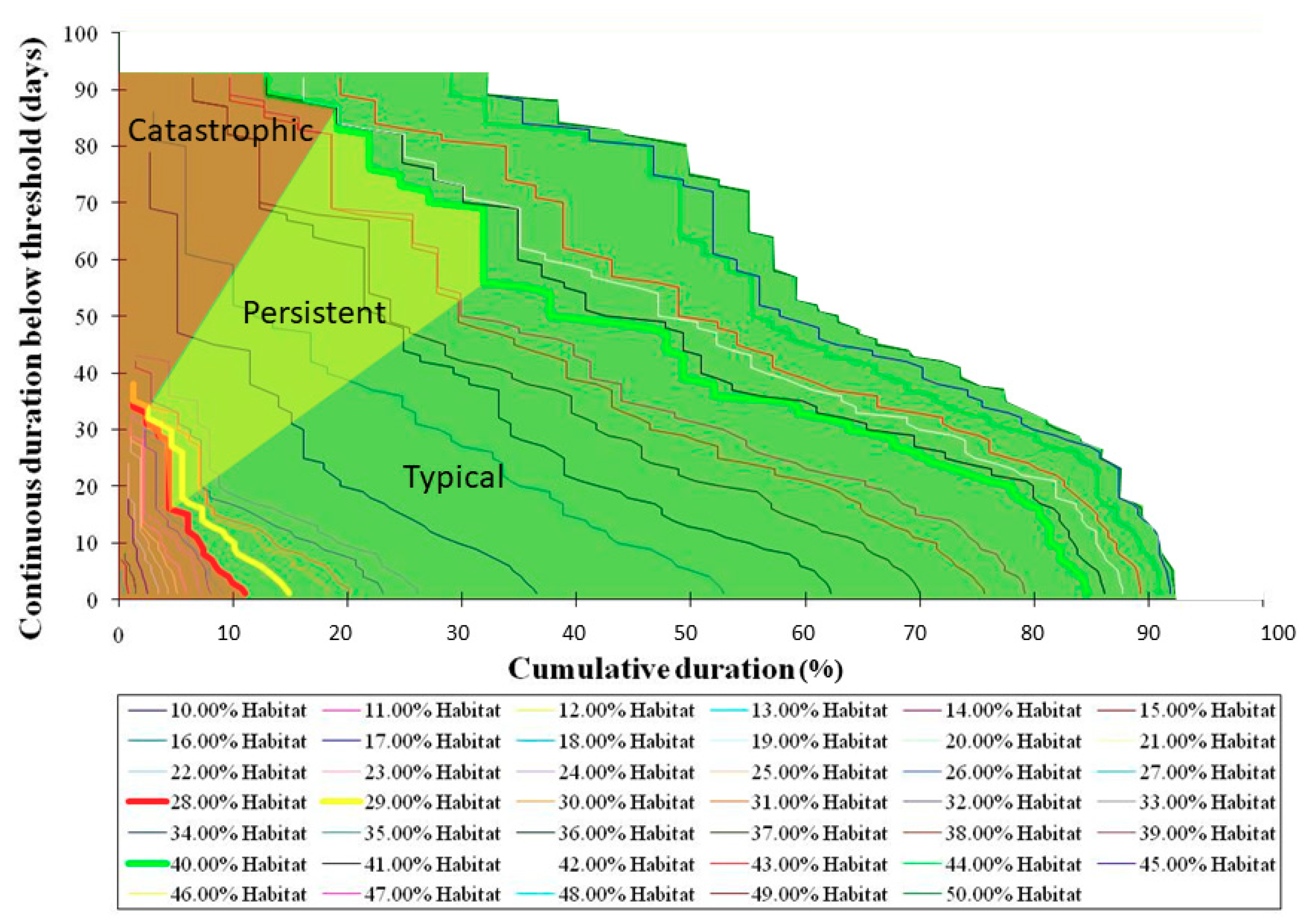
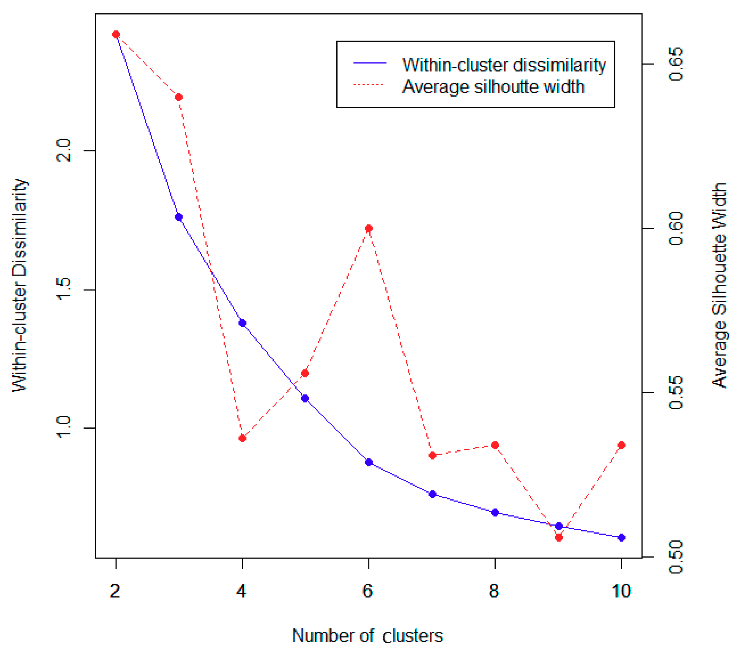
3. Results

Eight rearing and four spawning habitat-use guilds were specified for Poland (Appendix A, Table A1). Cluster analysis of rearing habitat guilds’ distribution data from 406 water bodies produced six fish ecological types of water bodies: Mountain rivers and streams, flysch rivers, lowland streams, lowland rivers, lake connectors with salmonids, and rivers connecting lakes, peat bogs, and estuaries. Figure 4 presents the scree plots of average within-cluster dissimilarities and average silhouette widths. The clusterwise Jaccard bootstrap mean indicated high cluster stability (>0.85) and ANOSIM documented their significance (R = 0.70 and p = 0.001).

Each fish ecological type of water body had an expected fish community structure for rearing and spawning bioperiods (Figure 5).

Due to a multitude of graphics created during the project, in the following section, only selected results are presented for the example of the Skawa River, which is representative of flysch rivers (type 2). Figure 6 demonstrates the example distribution of suitable habitats in the site for the lithophilic spawning guild that serves as an indicator species for the fall spawning bioperiod. It presents a substantial increase of suitable and optimal habitat areas with a flow increase.

Figure 7 shows an example of three habitat rating curves for each rearing and spawning bioperiod. Rearing and spawning habitat for the community increased rapidly and then levelled out at the flow of 1 L·s⁻¹·km⁻², while the rheophilic species spawning habitat increased continuously above the same threshold.

Figure 8 demonstrates UCUT curves calculated for the rearing habitat community. The curve representing 15% Channel Area (CA) of effective habitat was selected as a rare habitat threshold with four days of shortest persistent duration on the first critical point of the curve. The catastrophic duration (occurring not more often than every ten years) was selected with 16 days. The subsistence flow, corresponding with above habitat threshold was 1.03 L·s⁻¹·km⁻², which is equivalent to index p_b,s of 0.61. The critical habitat level was 16% CA, with 9 and 20 days as the shortest persistent and catastrophic durations, respectively. Corresponding trigger flow was equivalent to 1.24 L·s⁻¹·km⁻², which was equivalent to an index p_b,t of 0.74. The common habitat level was chosen at 20% CA, with 36 and 62 as shortest persistent and catastrophic durations, respectively. The corresponding base flow was 7.4 L·s⁻¹·km⁻², equal to an index p_b,c of 4.41. The lowest flow recorded of 0.166 L·s⁻¹·km⁻², equivalent to an index p_b,min of 0.1, was selected as the absolute minimum. The values for other bioperiods were obtained in similar ways and are presented in

Table 3. The eflow criteria calculated for the Skawa River; CA—Channel Area, I–XII—month.

Bioperiod	Spring Spawning	Rearing and Growth	Fall Spawning/Overwintering	Overwintering
Months	III–VI	V–IX	X–XII	I–II
Common habitat (% CA)	15.5	20	18	-
Shortest persistent duration (days)	22	36	27	32
Catastrophic duration (days)	36	62	51	42
Base flow (l·s−1·km−2)	5.8	7.4	6.6	5.5
Index pb,b	2.57	4.41	0.90	2.20
Critical habitat (% CA)	13	16	2	-
Shortest peristent duration (days)	7	9	8	8
Catastrophic duration (days)	15	20	14	32
Trigger flow (l·s−1·km−2)	2.59	1.24	1.55	2
Index pb,t	1.15	0.74	0.21	0.80
Rare habitat (% PK)	12.5	15	1	-
Shortest persistent duration (days)	6	4	6	8
Catastrophic duration (days)	11	16	7	12
Subsistence flow (l·s−1·km−2)	1.86	1.03	1.14	1.5
Index pb,s	0.82	0.61	0.16	0.60
Abs. Minimum flow (l·s−1·km−2)	0.725	0.166	0.518	0.414
Index pb,min	0.32	0.10	0.07	0.17

.

After performing the above analysis for every river, we calculated index p for all sampled rivers (

Table 4. FET specific coefficients p_b for all three thresholds. I–XII—month. Star symbol indicates rivers where no fall spawning occurs. 4s indicates type 4 with salmonid spawning.

FET	Threshold	Spring Spawning	Rearing and Growth	Fall Spawning/Overwintering	Overwintering
		III–VI	VII–IX (X)	X (XI)–XII	I–II
1	Base	0.65	0.87	0.83	1.77
	Critical	0.52	0.71	0.68	0.56
	Subsistence	0.46	0.56	0.60	0.52
2	Base	2.57	4.41	0.90	2.20
	Critical	1.15	0.74	0.21	0.80
	Subsistence	0.82	0.61	0.16	0.60
3 *	Base	4.08	3.83	4.56	1.62
	Critical	1.28	1.17	0.73	0.62
	Subsistence	1.04	0.85	0.55	0.37
4 *	Base	2.76	2.98	2.63	4.43
	Critical	1.03	0.93	0.75	0.74
	Subsistence	0.90	0.69	0.56	0.55
4s	Base	1.54	1.44	1.39	1.08
	Critical	1.11	0.95	0.85	0.89
	Subsistence	1.05	0.91	0.82	0.86

).

4. Discussion

This pilot project developed and demonstrated the conceptual assumptions of a proposed methodology for establishing regionally applicable eflows, extrapolating from site-specific habitat studies. This first work of its kind revealed practical obstacles facing the application of the proposed tools, but also demonstrated the feasibility of the overall concept. The study created a solid foundation for further adjustments and verification with additional data.

One of the key limitations of this study was the low number of RWBs that could be used for testing the approach. A complication in selecting RWBs was the uneven nature of the cluster sizes. For example, FET 3 low gradient small rivers and streams entailed 55% of Polish water bodies and FET 5 only 1%. Furthermore, it was preordained that seven RWBs would be investigated in this part of the study, and that each of them would be located in different regional water districts. Together with limited availability of hydrological data, this restricted our choices of water bodies. This was further limited by unforeseen circumstances than occurred during the study. For example, during the summer of 2015, the RWB on the Wierzyca River, representing FET 5, underwent substantial hydrological modification due to unregistered flow augmentation, and we were unable to complete the habitat survey. Furthermore, during the study, we also discovered that river Mienia suffered from flow alterations caused by channelization and melioration upstream of the RWB. The hydromorphologic survey of Mitręga River showed strong dominance of lowland river features (meanders, woody debris, and sandy bottom). Hence it raised the question if it was classified appropriately as belonging to FET 1. Therefore, for those two rivers, the habitat analysis was performed, but the results were not considered in defining FET specific eflows. Eventually, we were left with five RWBs to represent four FETs.

Furthermore, during the salmonid spawning bioperiod, we needed to consider FET 3 rivers, where these species occurred as a separate category. This was clearly visible on the p_b values for rivers Drawa and Świder, which were similar, except for the fall spawning season. Therefore, our preliminary eflow recommendations for the four investigated FETs were based on p_b values as presented in Table 4.

With the low number of samples, the variability of p_b within one FET, and therefore uncertainty could not be determined yet. It is a focus of a follow up study with a larger number of sites that is currently underway.

Another source of uncertainty that needs to be further investigated was introduced by inaccuracy of other components of the eflow formula, particularly the q_MBLF,k value for ungauged sites. This metric was traditionally applied in Poland, as it clearly represents the critical low flow time for the season. However, the formula for calculating runoff was not unique for the whole country and existing deviations could introduce additional variability. The accuracy of the metric estimates should be further tested, and if needed, it could be replaced by another flow metric.

Such research is necessary prior to implementation, as our goal is that the presented index p values, together with duration thresholds, can be used to calculate dynamic flow augmentation criteria for any location within the corresponding FET. These criteria could be applied to specify eflow management rules at this location.

Figure 9 demonstrates on the example of Skawa River how the above criteria could be applied at the surveyed location in the year 1988, which was a very dry year. The horizontal lines demonstrate the selected eflow levels. The proposed management rules are as follows:

(1)

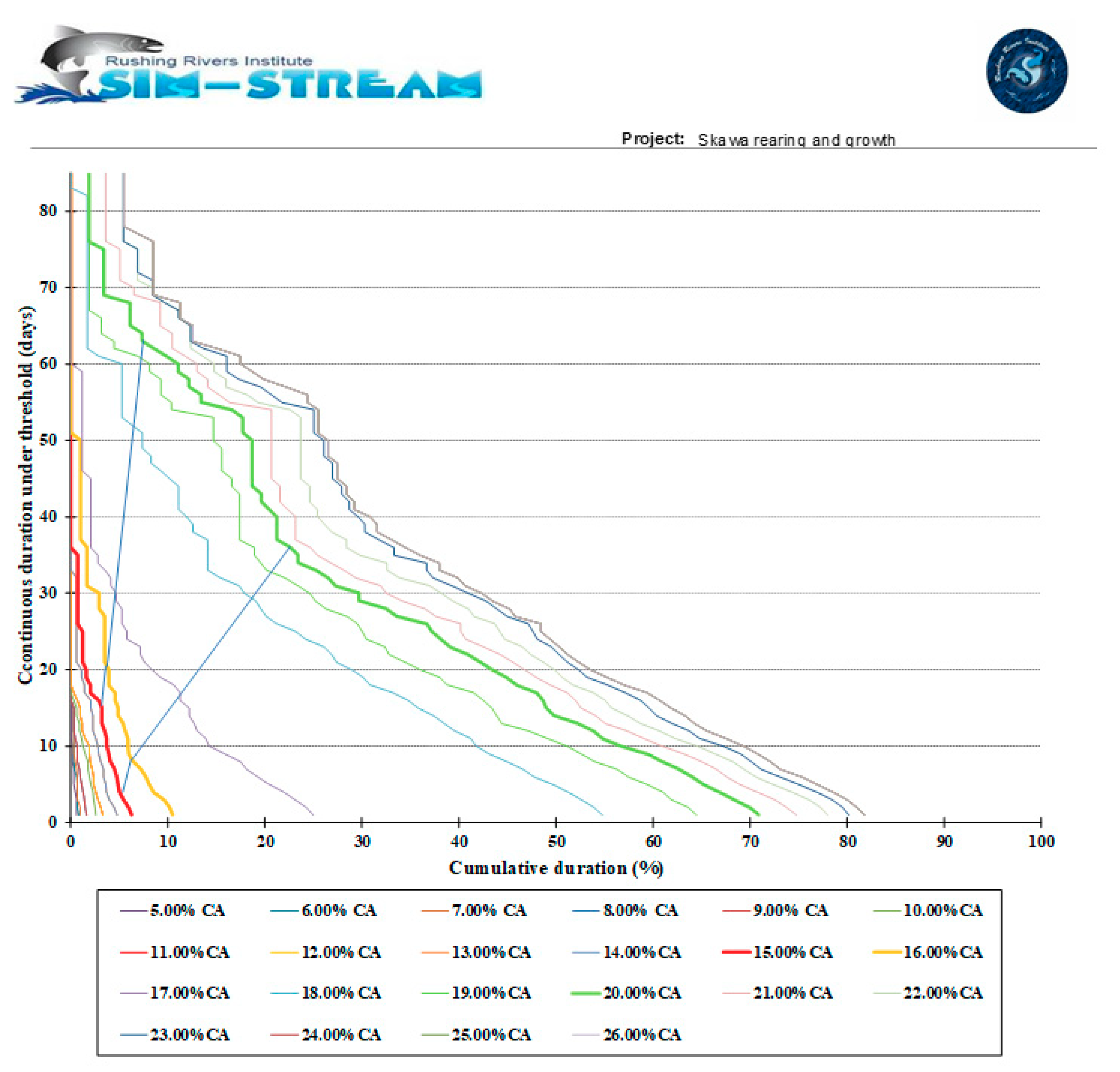
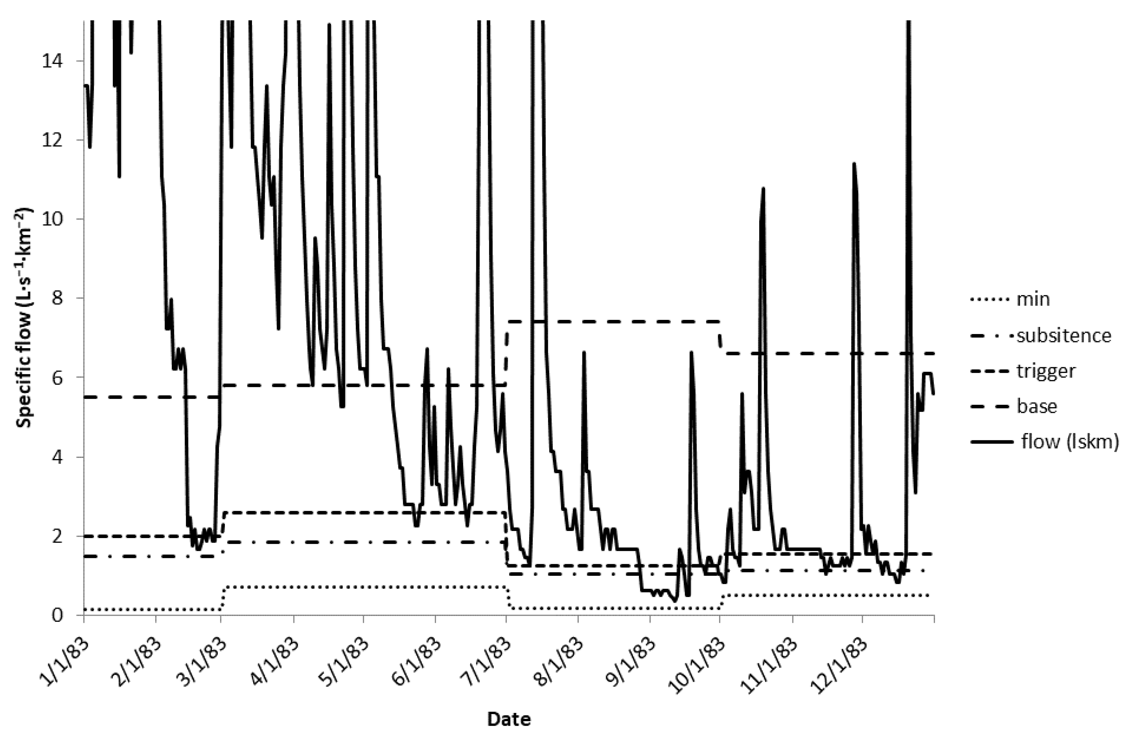
The absolute minimum flow line should never be crossed by the hydrograph;

(2)

The other three lines can be crossed, i.e., flows in the river become lower, but for durations shorter than the shortest persistent.

Otherwise, it is necessary to consider management actions, which consist of: passive continued observation, restriction of water withdrawals, flow augmentation, and/or morphologic modification. Passive continued observation can be permitted until the allowable duration has been exceeded more often than three times in the same bioperiod or catastrophic duration did not occur in the last ten years. Remaining mitigation measures aim to shorten the duration of habitat deficits and depend on local circumstances, such as augmentation water availability. Trigger flow criteria are triggering such actions. As presented in the diagram during overwintering and spring spawning, no action would be necessary. In rearing and growth bioperiods, flows went under the trigger threshold for a persistent period of 14 days; this could cause a preventive action (e.g., first level of withdrawal restrictions) if such a situation occurred two more times in this season. Otherwise, no action would be necessary. The fall spawning bioperiod began with a habitat deficit and after 29 days, it turned into a catastrophic duration. If there was no such deficit since 1978, no action would be necessary, but steps need to be taken to prevent it in the future.

Such dynamic management systems require continuous observation of flows at some control locations. This can consist of an adjacent gauge or gauge selected as representative for FET in the region. Alternatively, if such information is not available, one fixed eflow value could be established for a bioperiod using p_b for trigger flows. In such cases, flows falling below the trigger value would start management action. This is much easier to manage, but more costly in terms of water use.

It needs to be considered that the values presented here were developed using data from rivers with low hydromorphologic (HYMO) modification. Therefore, applying the same rules to rivers that are hydromorphologically modified may not bring the desired effect of maintenance of good ecological status. It is prudent to consider proposed eflow values valid only for rivers with low HYMO impact. An approach that would be applicable for hydromorphologically modified rivers still needs to be developed, and for the time being, we would recommend site-specific studies.

To summarize, the proposed approach is a first attempt to use habitat suitability models to justify eflow criteria on a large scale. At smaller regional scales, Vezza et al. [38] used MesoHABSIM to calculate minimum flow criteria for the Piedmont region of Italy. The development of generalized instream habitat models was also a significant step in that direction [39,40]; however, it did not fully represent regional instream flow guidelines. Similarly, establishing regional fish community types by Jowett and Richardson [41] served as a good conceptual foundation for our work. Our concept merely merged these and other ideas (e.g., Kostrzewa model) and used them for the purpose of setting biologically sound regional standards. The proof of concept and feasibility test was provided with our field studies, thus further verification is still required before implementation.

5. Conclusions

This paper presented a first of its kind conceptual approach for establishing e-flow rules, derived from detailed biological analysis through site specific habitat simulation models that are foundation for hydrological rule setting. On this path we utilized upscaling theory for extrapolation across biological and spatiotemporal scales [42]. We blended the concepts of guilds, bioperiods, geomorphic multiscale hierarchical framework, and specific flow duration analysis, hence using elements from multiple disciplines.

The advantage of the proposed approach is that it will allow for establishing protective flow rules that do not require intensive and expensive data collection for every development site. It is well suited for legal regulations at regional as well as global scale.

Offered framework is a good starting point for more detailed adjustments that will lead to incorporating the method into legal framework of e-flow regulation. The concept captures a complicated relationship between flows and biological response in one simple formula of universal utility and in this sense bears similarity to the Einstein’s equation cited in the title of this paper. Hence, this conceptual framework is not Poland specific, but can be applied worldwide regardless of regional characteristics. Obviously, the models require calibration with of a range of biological and physical data that may be regionally specific. Potential lack of data (i.e., waterbodies classification, fish fauna), occurring in some regions, could affect the model accuracy but not the logic of the framework. It is therefore our hope that river scientists and authorities worldwide will utilize this concept for better management and protection of riverine environments.

References

1. EEA—European Environmental Agency. European Waters—Assessment of Status and Pressures; EEA Report No 8/2012; European Environmental Agency: Copenhagen, Denmark, 2012. [Google Scholar] [CrossRef]
2. Bunn, S.E.; Arthington, A.H. Basic principles and ecological consequences of altered flow regimes for aquatic biodiversity. Environ. Manag. 2002, 30, 492–507. [Google Scholar] [CrossRef]
3. Rosenberg, D.M.; McCully, P.; Pringle, C.M. Global-scale environmental effects of hydrological alterations: Introduction. BioScience 2000, 50, 746–751. [Google Scholar] [CrossRef]
4. McKay, S.F.; King, A.J. Potential ecological effects of water extraction in small, unregulated streams. River Res. Appl. 2006, 22, 1023–1037. [Google Scholar] [CrossRef]
5. Ackerman, M.; Arthington, A.; Colloff, M.J.; Couch, C.; Crossman, N.D.; Dyer, F.; Overton, I.; Pollino, C.A.; Stewardson, M.J.; Young, W. Environmental flows for natural, hybrid, and novel riverine ecosystems in a changing world. Front. Ecol. Environ. 2014, 12, 466–473. [Google Scholar] [CrossRef] [Green Version]
6. Loar, J.M.; Sale, M.J.; Cada, O.F. Instream flow needs to protect fishery resources. In Proceedings of the Water Forum ’86: World Water in Evolution, Long Beach, CA, USA, 4–6 August 1986. [Google Scholar]
7. Poff, L.; Zimmerman, J.K. Ecological responses to altered flow regimes: A literature review to inform the science and management of environmental flows. Freshw. Biol. 2010, 55, 194–205. [Google Scholar] [CrossRef]
8. European Commission. Ecological Flows in the Implementation of the Water Framework Directive; Guidance Document No. 31. Technical Report 2015-086; European Commission: Brussels, Belgium, 2016; p. 108. [Google Scholar]
9. Pusey, B.J. Methods addressing the flow requirements of fish. In Comparative Evaluation of Environmental Flow Assessment Techniques: Review of Methods; Arthington, A.H., Zalucki, J.M., Eds.; LWRRDC Occasional Paper No. 27/98; LWRRDC: Canberra, Australia, 1998; pp. 66–105. [Google Scholar]
10. Poff, N.L.; Allan, J.D.; Bain, M.B.; Karr, J.R.; Prestegaard, K.L.; Richter, B.D.; Sparks, R.E.; Stromberg, J.C. The natural flow regime: A new paradigm for riverine conservation and restoration. BioScience 1997, 47, 769–784. [Google Scholar] [CrossRef]
11. Parasiewicz, P.; Rogers, J.; Larson, A.; Ballesterro, T.; Carboneau, L.; Legros, J.; Jacobs, J. Lamprey River Protected Instream Flow Report; Report for New Hampshire Department of Environmental Services, NHDES-R-WD-08-26; New Hampshire Department of Environmental Services: Concord, NH, USA, 2008; p. 980. [CrossRef]
12. Parasiewicz, P.; Thompson, D.; Walden, D.; Rogers, J.N.; Harris, R. Saugatuck River Watershed Environmental Flow Recommendations; Report for The Nature Conservancy and Aquarion; Rushing Rivers Institute: Amherst, MA, USA, 2010; p. 678. [Google Scholar]
13. Moore, M. Perceptions and Interpretations of Environmental Flows and Implications for Future Water Resource Management: A Survey Study. Master’s Thesis, Department of Water and Environmental Studies, Linköping University, Linköping, Sweden, 2004. [Google Scholar]
14. Richter, B.D.; Baumgartner, J.V.; Wigington, R.; Braun, D.P. How much water does a river need? Freshw. Biol. 1997, 37, 231–249. [Google Scholar] [CrossRef]
15. Harby, A.; Baptist, M.; Dunbar, M.J.; Schmutz, S. State-of-the-Art in Data Sampling, Modelling Analysis and Applications of River Habitat Modelling; Final Report; Action COST: Brussels, Belgium, 2004; p. 626. [Google Scholar]
16. Tharme, R.E. A global perspective on environmental flow assessment: Emerging trends in the development and application of environmental flow methodologies for rivers. River Res. Appl. 2003, 19, 397–441. [Google Scholar] [CrossRef]
17. Kostrzewa, H. Weryfikacja Kryteriów i Wielkości Przepływu Nienaruszalnego dla Rzek Polski [Verification of Criteria and Magnitude of Untouchable Flows for Polish Rivers]; Mat. Badawcze, Seria: Gospodarka Wodna i Ochrona Wód; IMGW: Warszawa, Poland, 1977. (In Polish) [Google Scholar]
18. Bain, M.B.; Meixler, M.S. A target fish community to guide river restoration. River Res. Appl. 2008, 24, 453–458. [Google Scholar] [CrossRef]
19. Gurnell, A.M.; Rinaldi, M.; Belletti, B.; Bizzi, S.; Blamauer, B.; Braca, G.; Buijse, A.D.; Bussettini, M.; Camenen, B.; Comiti, F.; et al. A multi-scale hierarchical framework for developing understanding of river behaviour to support river management. Aquat. Sci. 2016, 78, 1–16. [Google Scholar] [CrossRef] [Green Version]
20. Parasiewicz, P. MesoHABSIM: A concept for application of instream flow models in river restoration planning. Fisheries 2001, 26, 6–13. [Google Scholar] [CrossRef] [Green Version]
21. Parasiewicz, P. The MesoHABSIM model revisited. River Res. Appl. 2007, 23, 893–903. [Google Scholar] [CrossRef]
22. European Commission. Common Implementation Strategy for the Water Framework Directive (200/60/EC). Guidance Document No. 2. Identification of Water Bodies; Office for Official Publications of the European Communities: Luxembourg, 2003; p. 23. Available online: https://circabc.europa.eu/sd/a/655e3e31-3b5d-4053-be19-15bd22b15ba9/Guidance%20No%202%20-%20Identification%20of%20water%20bodies.pdf (accessed on 1 October 2018).
23. ISAP. Dz.U. 2011 nr 258 poz. 1549. Rozporządzenie Ministra Środowiska z Dnia 9 Listopada 2011 r. w Sprawie Klasyfikacji Stanu Ekologicznego, Potencjału Ekologicznego i Stanu Chemicznego Jednolitych Części Wód Powierzchniowych. Available online: http://prawo.sejm.gov.pl/isap.nsf/DocDetails.xsp?id=WDU20112581549 (accessed on 1 October 2018).
24. Prus, P.; Adamczyk, M.; Buras, P.; Wiśniewolski, W. Metody Oceny Stanu Środowiska Rzek w Oparciu o Ichtiofaunę [Fish-Based Methods for River Ecological Status Assessment]; Ciecierska, H., Dynowska, M., Eds.; Biologiczne Metody Oceny Stanu Środowiska, T. II. Ekosystemy Wodne [Biological Methods for Environment Status Assessment. Part II. Water Ecosystems]; Mantis: Olsztyn, Poland, 2013; pp. 199–236. ISBN 978-83-62860-19-7. (In Polish) [Google Scholar]
25. Prus, P.; Wiśniewolski, W. (Eds.) Monitoring Ichtiofauny w Rzekach. Przewodnik Metodyczny [Ichthyofauna Monitoring in Rivers. Methodological Guide]; Biblioteka Monitoringu Środowiska, Główny Inspektorat Ochrony Środowiska: Warszawa, Poland, 2013; 72p. Available online: http://www.gios.gov.pl/images/dokumenty/pms/monitoring_wod/Przewodnik_metodyczny_do_oceny_rybnej_rzek.pdf (accessed on 18 October 2018). (In Polish)
26. Leonard, P.M.; Orth, D.J. Use of habitat guilds of fishes to determine instream flow requirements. N. Am. J. Fish. Manag. 1988, 8, 399–409. [Google Scholar] [CrossRef]
27. Welcomme, R.L.; Winemiller, K.O.; Cowx, I.G. Fish environmental guilds as a tool for assessment of ecological condition of rivers. Rivers Res. Appl. 2006, 22, 377–396. [Google Scholar] [CrossRef]
28. Kaufman, L.; Rousseeuw, P.J. Findings Groups in Data. An Introduction to Cluster Analysis; Wiley and Sons: Hoboken, NJ, USA, 2009; p. 349. [Google Scholar]
29. McGarigal, K.; Cushman, S.A.; Stafford, S.G. Multivariate Statistics for Wildlife and Ecology Research; Springer: New York, NY, USA, 2000. [Google Scholar]
30. Hennig, C. Cluster-Wise Assessment of Cluster Stability. Comput. Stat. Data Anal. 2007, 52, 258–271. [Google Scholar] [CrossRef]
31. R Core Team. R: A Language and Environment for Statistical Computing; R Foundation for Statistical Computing: Vienna, Austria, 2014; Available online: http://www.R-project.org/ (accessed on 1 October 2018).
32. Rushing Rivers Institute. SimStream: A MesoHABSIM Simulation Software. 2014. Available online: www.Sim-stream.org (accessed on 1 October 2018).
33. Parasiewicz, P.; Pegg, M.; Rogers, J.R.; Behmer, A.; Eldridge, A. Developing Environmental Flows for Fish and Wildlife: A Mesohabitat Study on the Niobrara River; Rushing Rivers Institute and University of Nebraska Lincoln: Lincoln, NE, USA, 2014; p. 98. [Google Scholar]
34. Parasiewicz, P. Using MesoHABSIM to develop reference habitat template and ecological management scenarios. River Res. Appl. 2007, 23, 924–932. [Google Scholar] [CrossRef]
35. Lake, P. Disturbance, patchiness, and diversity in streams. J. N. Am. Benthol. Soc. 2000, 19, 573–592. [Google Scholar] [CrossRef]
36. Parasiewicz, P. Habitat time series analysis to define flow augmentation strategy for the Quinebaug River, Connecticut and Massachusetts, USA. River Res. Appl. 2008, 24, 439–452. [Google Scholar] [CrossRef]
37. Parasiewicz, P.; Rogers, J.N.; Gortazar, J.; Vezza, P.; Wiśniewolski, W.; Comoglio, C. The MesoHABSIM Simulation Model—Development and applications. In Ecohydraulics: An Integrated Approach; Maddock, I., Harby, A., Kemp, P., Wood, P., Eds.; John Wiley & Sons Ltd.: Hoboken, NJ, USA, 2014; pp. 109–124. [Google Scholar]
38. Vezza, P.; Parasiewicz, P.; Spairani, M.; Comoglio, C. Habitat modeling in high gradient streams: The mesoscale approach and application. Ecol. Appl. 2014, 24, 844–861. [Google Scholar] [CrossRef] [PubMed]
39. Lamouroux, N.; Jowett, I. Generalized instream habitat models. Can. J. Fish. Aquat. Sci. 2005, 62, 7–14. [Google Scholar] [CrossRef]
40. Lamouroux, N.; Capra, H. Simple predictions of instream habitat model outputs for target fish populations. Freshw. Biol. 2002, 47, 1543–1556. [Google Scholar] [CrossRef]
41. Jowett, I.G.; Richardson, J. Fish communities in New Zealand rivers and their relationship to environmental variables. N. Z. J. Mar. Freshw. 2003, 37, 347–366. [Google Scholar] [CrossRef] [Green Version]
42. Parasiewicz, P. Upscaling: Integrating habitat model into river management. Can. Water Resour. J. 2003, 28, 283–300. [Google Scholar] [CrossRef]
Figure 1. Scheme of eflow determination process. HUG stands for habitat-use guilds, TFC for target fish community, HYMO for hydromorphology, NHC for nonhierarchical cluster analysis, MSHF for multiscale hierarchical framework, Coeff P for coefficient p.
Water 10 01501 g001
Figure 2. Map of sampling locations distribution in Poland.
Water 10 01501 g002
Figure 3. Example of uniform continuous under-threshold curves for determination of HST. Each curve on the diagram represents the cumulative duration of events when habitat is lower than a threshold (X-axis) for a continuous duration of days depicted on the Y-axis.
Water 10 01501 g003
Figure 4. Scree plot of k-means clustering for average within-cluster dissimilarities and average silhouette widths.
Water 10 01501 g004
Figure 5. FET-specific expected fish community structures.
Water 10 01501 g005
Figure 6. Maps of suitable habitat areas for the Skawa River (lskm stands for L·s−1·km−2).
Water 10 01501 g006
Figure 7. Habitat rating curves for bioperiod-specific fish communities in the Skawa River.
Water 10 01501 g007
Figure 8. UCUT curves for fish communities present during the rearing bioperiod.
Water 10 01501 g008
Figure 9. Flows recorded at the gauge of the Skawa River in 1983 together with flow thresholds.
Water 10 01501 g009