Optimal Design of Circular Baffles on Sloshing in a Rectangular Tank Horizontally Coupled by Structure

Abstract

Parametric studies on the optimization of baffles on vibration suppression of partially filled tanks coupled by structure have been widely conducted in literature. However, few studies focus on the effect of the position of the baffles on fluid flow stratification and dampening the motion. In the present study, a numerical investigation, an engineering analysis, and optimal design study were performed to determine the effect of external flow on circular obstacle baffles performance on suppressing the vibrations of coupled structure in a closed basin. The single degree of freedom model (mass–spring–damper) is used to model the structure that holds the tank. The coupled system is released from an initial displacement without a velocity. The governing mass, turbulent Navier–Stokes momentum, volume of fluid, and one degree of freedom structure equations are solved by the Pressure-Implicit with Splitting of Operators algorithm in fluids and Newmark method in structure. Based on a detailed study of transient structure motion coupled with sloshing dynamics, the optimal baffle location was achieved. Optimal position of the baffle and its width are systematically obtained with reference to the quiescent free surface.

1. Introduction

The effect of fluid–solid interaction has been studied in recent years [1,2,3,4,5,6]. Interaction of two-phase flows and porous media [7], breaking and non-breaking long waves with offshore [8,9], interaction of boiling and structure [10], natural convection and elliptical structures [11], Kelvin instability [12,13,14], Rayleigh–Taylor instability [15], and bursting of the recirculation on structure [16,17]. Among them, suppression of liquid sloshing in rigid tanks [18] is needed in many engineering applications such as nuclear waste container, liquid contained space vehicles [19], aircraft with liquid fuels [20], cargo tanks [21,22], elevated water tanks [23], etc. [24]. The sloshing phenomena is important in two-phase cryogenic fluid storage [19,25], Liquid-Hydrogen Tank [18,20,23,26], oxygen tank in space shuttle [24,27], cryogenic Liquefied Natural Gas (LNG) ship tanks [28,29,30], liquid hydrogen tank [31,32], slosh baffle in propellant tank [33,34,35,36,37,38], anti-slosh baffles in circular tanks [21], vertical baffles in elliptical tanks [22], pressurization of a large scale cryogenic storage tank [39], subcooled boiling [40], and sloshing control [41,42,43,44,45]. One of the passive solutions to this problem is Baffle structures [33]. They are extremely powerful in moderating solid shaking of fluid when the tank is affected by a sudden outside power. NASA [23] was one of the first to research the steadiness of a sloshing under parametric excitation utilizing trial and hypothetical means. As per this hypothesis, specific modes will be energized for a particular blend of abundancy and recurrence as anticipated by the soundness outline. Yoon [20] has observed soak standing waves to be steady under consonant irritation yet precarious under sub-symphonious excitation. It should be pointed out that, under FSI coupled excitation, non-straight particular coordinated efforts support the essentialness trade process from the empowered modes to various modes [20]. Hasheminejad [21] have demonstrated that the out-of-stage modes are more steady than in-stage modes even with little disorders. Kannapel et al. [24] used Computational Fluid Dynamics (CFD) to investigate and have investigated the slosh conduct in a hoisted water tower, and the framework was seen to show hard non-straight conduct under parametrically energized first transverse two-dimensional sloshing mode. The Baffle structures are exceptionally successful in moderating all of these looks into demonstrating the essential parts of confuses in tank configuration to diminish sloshing and also relieve affect power to the supporting structure of the tank. In contrast with conventional work based techniques, Ma [31] was interested in catching the position of the programmed free surface. To this end, techniques, for example, Smooth Particle Hydrodynamics (SPH), Meshless Local Petrov–Galerkin (MLPG), have been prevalently utilized [30]. Panzarella [19] has presented that Reynolds put the middle value of the fierce model into the SPH system to reproduce fluid sloshing in a rectangular tank under intermittent flat excitation. Behruzi [28] have gotten smooth and precise weight fields on tank dividers in a 2D sloshing issue with an enhanced powerful strong limit treatment in a blend with moving slightest square estimation. Adam [26] has built up a two-stage SPH strategy with an enhanced strong limit treatment to mimic sloshing in a water tank and related liquid structure connection impacts. Grayson [29] has utilized a Meshless Local Petrov–Galerkin (MLPG) technique with a moving minimum square (MLS) estimate to examine sloshing in a 2D kaleidoscopic tank. These reproductions were additionally stretched out to think about the free surface motions in a fluid filled composite compartment in two-measurements. Lately, Ref. [41] aptly condenses parametric sloshing—specifically, the ongoing endeavors to comprehend and foresee design determination utilizing numerical and scientific instruments. The impact of damping on steadiness and non-customary wellsprings of excitation were additionally examined. They established an $\mu$ outline with a model decrease connected to the subsequent controller. The second one is a settled structure controller ’hearty systune’ included, which executes the calculation from the work of Apkarian [41]. This last procedure is extremely alluring, seeing that it permits determining a powerful controller for endorsed controller topologies. Be that as it may, the parametric organized plan, which limits the most pessimistic scenario $H_{\infty }$ standard, depends on non-smooth streamlining. This can prompt substantial, unexpected changes in the controller parameters for even little changes in the weighting capacity, which oppose the instinct. A full request $\mu$ controller is in this way decent at managing, important for filling in as a benchmark.

The flow around a circular cylinder is studied in the works of [46,47,48,49,50,51,52,53,54,55]. The scientists used various formulations to simulate the phenomena. Girimaji used a Pressure–Strain correlation [56,57], Reynolds Stress Closure Equations [58], and Partially-Averaged Navier–Stokes Model [59,60,61]. It is known that the Surface-Roughness can affect the mean flow past circular cylinder [46,62]. Other models that were used to simulate the flow around a circular cylinder are $k-ϵ$ Model [63], Organized Wave [64], Stochastic Backscatter Model [65], Scale-Resolving Models [66], Large Eddy Simulation (LES) [67], Smagorinsky Homogeneous and Isotropic Turbulence [68], Incompressible Homogeneous Turbulence [69], Vortex method [70,71], $k-\omega$ [72], Multiple-Time-Scale Modeling [73,74], Partially Integrated Transport Model [75], Effective-Viscosity [76], the RANS-LES Approach [77,78,79], Pressure-Strain Correlation Modeling [80,81,82], Shear Stress Transport (SST) Turbulence Model [83], Reynolds-Stress Turbulence Closure [84,85], etc. The phenomena were studied flow around a circular cylinder are Three-Dimensional Patterns of Streamwise Vorticity [86,87,88,89,90], Influence of Aspect Ratio [91,92,93], Laser Doppler Velocimetry (LDV)-Measurements [94], Pressure Distributions [95], Fluctuating Lift [96], Reynolds Number Effects on the Flow and Fluid Forces [97,98,99], Instability [100,101], Structure of the Near Wake Shear Layer [102,103,104], Equilibrium of an Incompressible Heavy Fluid of Variable Density [105], Non-Newtonian Fluids [106], and Control of a Cylinder Wake [107]. A direct comparison between volume and surface tracking methods shows that the centered finite differences at the high Reynolds number fails and it will not converge even with mesh refinement [108]. Generally, Front Tracking converges faster than Volume Tracking in the liquid–air interfaces [109]. There are some classical reviews papers on turbulence modeling and high-resolution simulations. Specifically, there is a review on turbulence modeling and turbulent-flow computation in aeronautics by Leschziner et al. [110] and on Large Eddy Simulation with high Order resolution methods by Drikakis et al. [111].

Based on the above literature search, there is an absence of study on the effect of pipe shaped baffles on the fluid flow in the rigid tank coupled with structure. The aim of the current study is to investigate the effect of the presence of pipe shaped baffles in the tank on the fluid flow around it and the effect of different immersing of the baffles as well as the liquid fill levels on the free surface profiles and vibration mitigating behavior of fluid sloshing on coupled motion.

2. Mathematical Model

Setup

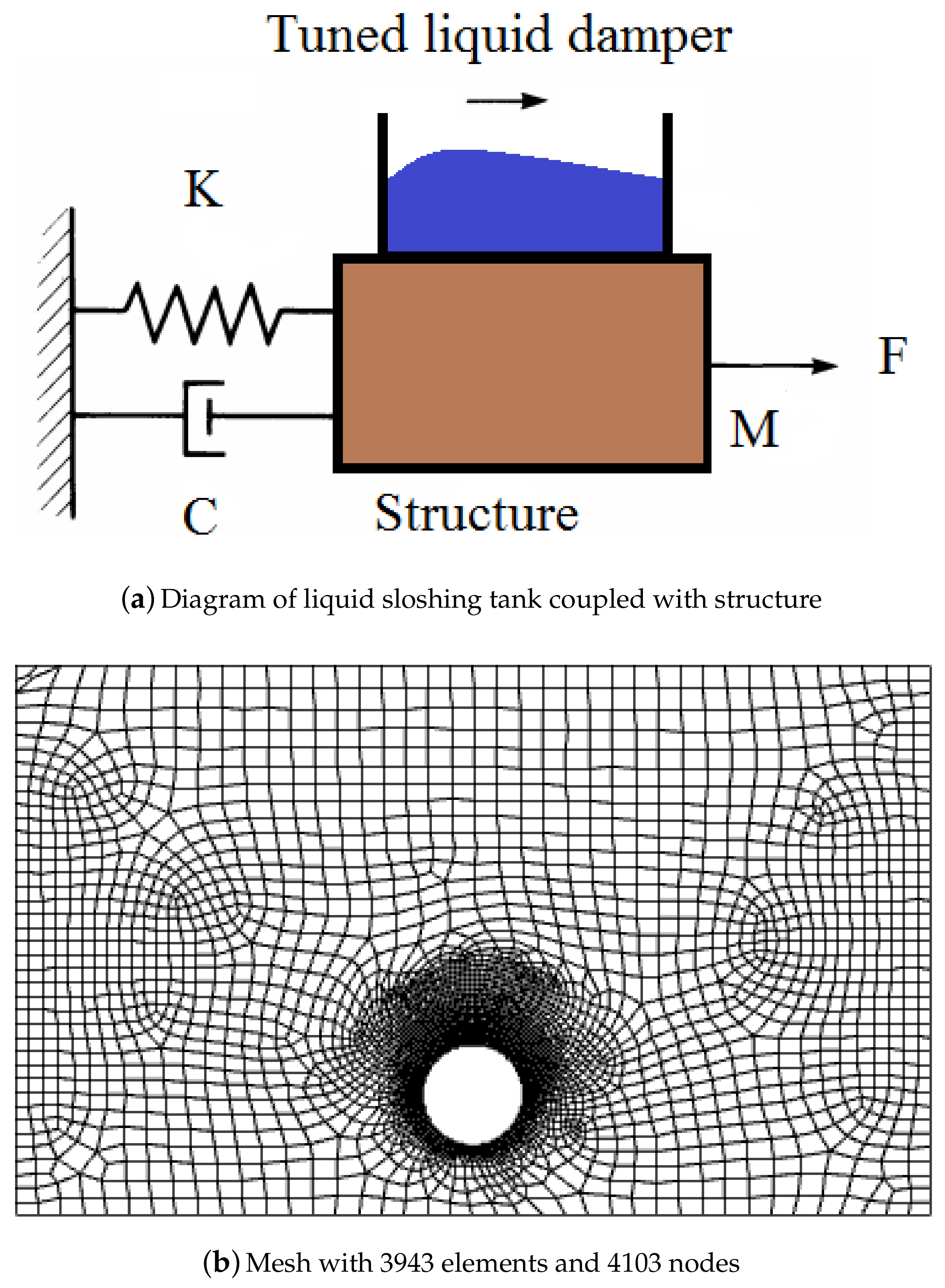
Consider a partially filled tank in 2D rectangular shape as shown in Figure 1b with the maximum height of 300 mm and the length of 500 mm, respectively. For the basic case (without baffles), the filling ratio is considered to be 110 mm. The fluid density ($\rho$) is considered constant in all simulations. All numerical studies done in this research are summarized in

Table 1. Simulations executed in this paper.

Parameters	Group of Setups
Fill level	6 cm, 11 cm, 20 cm
Distance from left	10 cm, 25 cm
Gap	1 cm, 2 cm, 3 cm, 5 cm, 10 cm

. For the incompressible fluid, the governing equations are

$$\frac{\partial \langle V_i\rangle }{\partial x_i}=0,$$

(1)

which is continuity equation adopted by $\rho =const$ in $\frac{\partial \rho }{\partial t}+\nabla ·\left(\rho \mathbf{u}\right)=\mathbf{0}$ and

$$\frac{\partial \langle V_i\rangle }{\partial t}+\langle V_j\rangle \frac{\partial \langle V_i\rangle }{\partial x_j}=-\frac{1}{\rho }\frac{\partial \langle P\rangle }{\partial x_i}+\nu \frac{{\partial }^2\langle V_i\rangle }{\partial x_j\partial x_j}+\frac{1}{\rho }\frac{\partial \tau \left(V_i,V_j\right)}{\partial x_j}+\mathbf{f},$$

(2)

which is the momentum equation adopted by $\mathsf{\Phi }\equiv \langle \mathsf{\Phi }\rangle +\varphi$ (for variables, Cartesian velocity components $V_i$ and pressure (P)) in $\rho \frac{\mathrm{D}\mathit{u}}{\mathrm{D}t}=-\nabla \mathbf{p}+\mu \Delta \mathbf{u}+\rho \mathbf{f}$. In Equation (2), the generalized central second moment $\tau (V_i,V_j)$ is the sub-grid stresses tensor related to strain-rate tensor ($\langle S_{ij}\rangle =\frac{1}{2}\left(\frac{\partial \langle V_i\rangle }{\partial x_j}+\frac{\partial \langle V_j\rangle }{\partial x_i}\right)$,) by one-point Boussinesq closure:

$$\frac{{\tau }_{ij}(V_i,V_j)}{\rho }=2\nu \langle S_{ij}\rangle -\frac{2}{3}k{\delta }_{ij},$$

(3)

where ${\delta }_{ij}$ is the Kronecker delta, and $\nu$ is the turbulent viscosity (eddy)

$$\nu =\frac{k}{\omega },$$

(4)

($nu=C_{\mu }\frac{k^2}{ϵ}$ if k-$ϵ$ model is used for the turbulence) and turbulence kinetic energy (k) is found from

$$\frac{Dk}{Dt}={\tau }_{ij}\frac{\partial \langle V_i\rangle }{\partial x_j}-{\beta }^{*}k\omega +\frac{\partial }{\partial x_j}\left[\left(\nu +\nu {\sigma }_k\frac{f_{\omega }}{f_k}\right)\frac{\partial k}{\partial x_j}\right],$$

(5)

$$\frac{D\omega }{Dt}=\frac{\alpha }{\nu }{\tau }_{ij}\frac{\partial \langle V_i\rangle }{\partial x_j}-\left(\alpha {\beta }^{*}-\frac{\alpha {\beta }^{*}}{f_{\omega }}+\frac{\beta }{f_{\omega }}\right){\omega }^2+\frac{\partial }{\partial x_j}\left[\left(\nu +\nu {\sigma }_{\omega }\frac{f_{\omega }}{f_k}\right)\frac{\partial \omega }{\partial x_j}\right].$$

(6)

The coefficients are the same as [74,83]. The $k^{3/2}/ϵ$ and Kolmogorov length scale ${\left(\frac{{\left({\nu }_t+\nu \right)}^3}{ϵ}\right)}^{1/4}$ are two measures of the grid size.

The method of the volume of fluid is used to model the free surface of the fluid [34,39]. The method computes the phase fraction $\alpha$ ($\alpha =1$ means pure liquid and $\alpha =0$ means pure gas since $\sum {\alpha }_i=1$) through the domain by solving the material derivative of $\alpha$ equals zero as

$$\frac{\partial \langle {\alpha }_i\rangle }{\partial t}+\langle V_j\rangle \frac{\partial \langle {\alpha }_i\rangle }{\partial x_j}=0.$$

(7)

The surface tension source term in Equation (2) ($\mathbf{q}$ by continuum surface force model) is found from

$$\mathbf{f}=\sum _{\mathbf{i}<\mathbf{j}}{\sigma }_{\mathbf{ij}}\frac{{\alpha }_{\mathbf{i}}{\rho }_{\mathbf{i}}{\kappa }_{\mathbf{j}}\nabla {\alpha }_{\mathbf{j}}+{\alpha }_{\mathbf{j}}{\rho }_{\mathbf{j}}{\kappa }_{\mathbf{i}}\nabla {\alpha }_{\mathbf{i}}}{\frac{\mathbf{1}}{\mathbf{2}}({\rho }_{\mathbf{i}}+{\rho }_{\mathbf{j}})},$$

(8)

where surface tension is $\sigma =0.076$ N/m and $\kappa$ is defined in terms of the divergence of the surface normal ($\kappa =\nabla ·n=\nabla ·\nabla \alpha$).

The coupling equation between the fluid and solid shown in Figure 1b is

$$m\ddot{x_s}+c\dot{x_s}+k{x}_s\equiv \frac{\rho gW}{2}\left(h_{x=L}^2-h_{x=0}^2\right).$$

(9)

The flow regime around pipes is detected based on some parameters such as bulk fluid turbulence intensity and aspect ratio. The most important parameter is the Reynolds number,

$$Re\equiv \frac{{\overline{V}}_{\infty }D}{\nu },$$

(10)

where D is the pipe diameter, ${\overline{V}}_{\infty }$ is the time-averaged velocity, and $\nu$ is the effective fluid kinematic viscosity (see

Table 2. Reynolds number and the flow regime around pipes.

Flow Regimes
fully laminar	$Re$ < 180–200
transition in the wake	$Re$ < 350–400
transition in the free shear-layer	$Re<1.0\times {10}^5–2.0\times {10}^5$
transition in the boundary-layer	$Re<2\times {10}^5–5.0\times {10}^6$
fully turbulent boundary-layer	$Re>5\times {10}^6$

). Based on the data provided for set-up, the Reynolds number of the whole tank is in the transition in the boundary-layer flow regime while the Reynolds number of the pipe is in the transition in the free shear-layer flow regime around pipes.

The kinematic (no mass flux across the free surface)

$$\frac{\partial \eta }{\partial t}+\langle V_j\rangle .\frac{\partial \eta }{\partial x_j}=0$$

(11)

and dynamic (dynamic equilibrium of free surface)

$$\Delta P=\sigma \times \frac{\partial V_1}{\partial x_2}$$

(12)

are free surface boundary conditions and wall boundary conditions are no-slip velocity,

$$\mathbf{u}·\mathbf{n}=0,$$

(13)

where $\mathbf{n}$ is the unit normal vectors to the walls.

3. Results and Discussion

3.1. Validation and Grid Independence

Pressure implicit method with splitting of operators [112] is used for the solution of the system of Partial Differential Equations (PDEs) appearing in Equations (1), (2), (5)–(7) and (9). The three-step method (predictor–corrector–regularization), first by a guessed pressure ($\nabla p$), finds turbulent velocity field via iterative resolution techniques

$$a_P{\mathbf{u}}_P=-\sum _N{a}_N{\mathbf{u}}_{\mathbf{N}}+{\mathsf{\Phi }}_{previous}\left({\mathbf{u}}_{previous}\right)-\nabla p=\mathsf{\Phi }\left(\mathbf{u}\right)-\nabla p$$

(14)

and then corrects pressure, and finds corresponding velocity components (satisfy $\nabla ·\mathbf{u}=0$) with the Poisson equation:

$$\nabla ·\left(\frac{\nabla p}{a_P}\right)=\nabla ·\left(\frac{\mathsf{\Phi }\left(\mathbf{u}\right)}{a_P}\right)=\sum _{f}S\times {\left(\frac{\mathsf{\Phi }\left(\mathbf{u}\right)}{a_P}\right)}_f.$$

(15)

Finally, in the regularization step, by putting the difference of the corrected and guessed pressure values in the momentum equation, correction of the velocity can be determined.

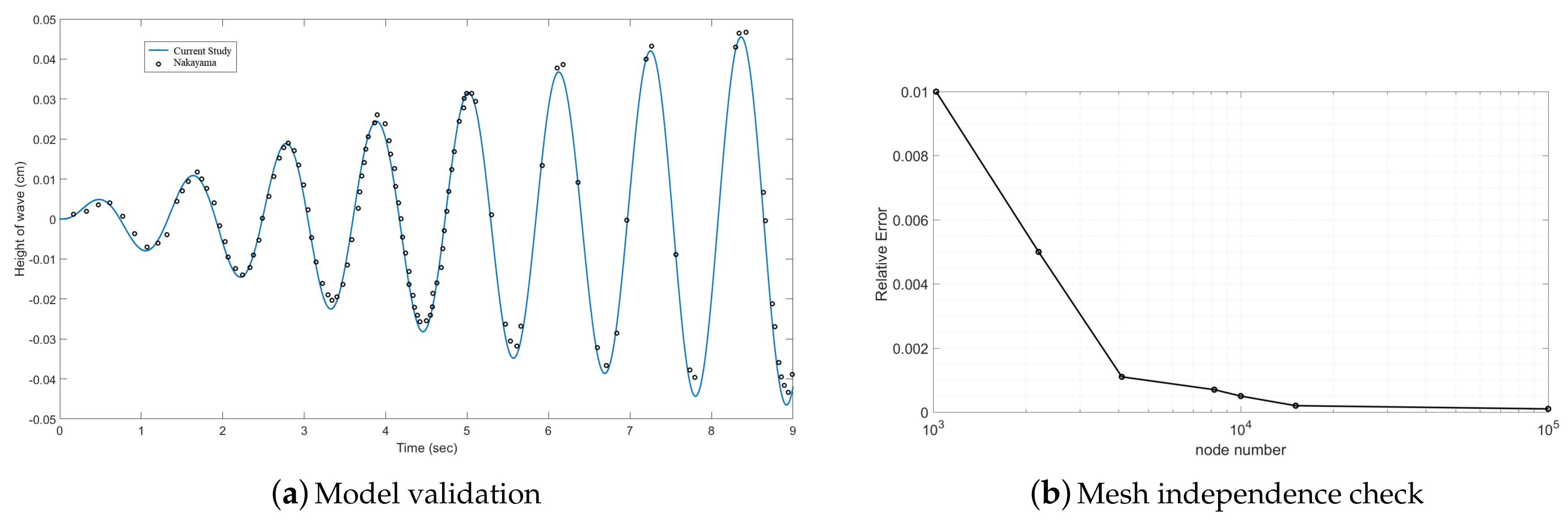
The problem shown in Figure 1b with parameters of

Table 3. Structure parameters.

Parameter	Value
Mass	18.9 kg
Natural frequency	1.09 1/s
Damping ratio	0.0019

is solved by various mesh sizes. The approach outlined above would be true if it has small error for the given mesh and one can make sure that the solution is also independent of the mesh resolution. The convergence based on average of the Root Mean Square (RMS) Error values over the domain compared with ${10}^5$ nodes was performed. The ${10}^5$ nodes solution is used as the smallest mesh that gives the mesh independent solution. The results are summarized in Figure 2a. Because the solution is not changing significantly with the refinement of mesh from ${10}^4$ nodes to ${10}^5$ nodes, we have achieved a mesh independent solution. You need to refine the mesh more, and repeat the process until you have a solution that is independent of the mesh. You should always do this (to reduce your simulation run time).

The vessel motion is $X_s$, which is defined as

$$X_s=0.002sin(5.5t)$$

(16)

in [35]. The outcomes appeared in Figure 2a shows that the numerical simulation here has a good agreement with the Finite Element Method (FEM) benchmark results. The code will develop quickly with high precision when Courant number is equivalent to 0.5, speaking to a generally extensive time step. Figure 2b is the grid accuracy check of work. A reasonable accuracy can be seen between 8 K work and 10 K work in the calculation of structure location under the same conditions, while the contrast between 10 K work and 12 K work can be disregarded. With respect to utilization of calculation assets, a 10 K element number with $Co=0.5$ is used for other cases. In this manner, all recreations worked and there is an element number of around 10 K. Convergence for a Steady State simulation satisfies the following three conditions: Residual RMS Error values have reduced to an acceptable value (typically ${10}^{-4}$), monitor points for our values of interest have reached a steady solution, and the domain has imbalances of less than one percent. Here, the converging criteria for fierce continuity equation is ${10}^{-7}$, for momentum equation is ${10}^{-7}$, and for turbulence equations (dissipation and energy rates) are ${10}^{-5}$. In turbulent flows, there is a considerable challenge in error control, especially of the near-wall boundary condition. As the wall-functions are used in the near-wall boundary layer, the size of the near-wall cell is limited [113]. The low Reynolds model causes a very large number of nodes at the near wall boundary layer. Other than spatial error, in transient turbulent flow calculations, the temporal errors appeared. The temporal error of each step is proportional to $\Delta t^2$ other than a Courant–Friedrick limit (CFL) used for numerical stability for the time advancement [114].

3.2. Effect of Gap with the Bottom Wall

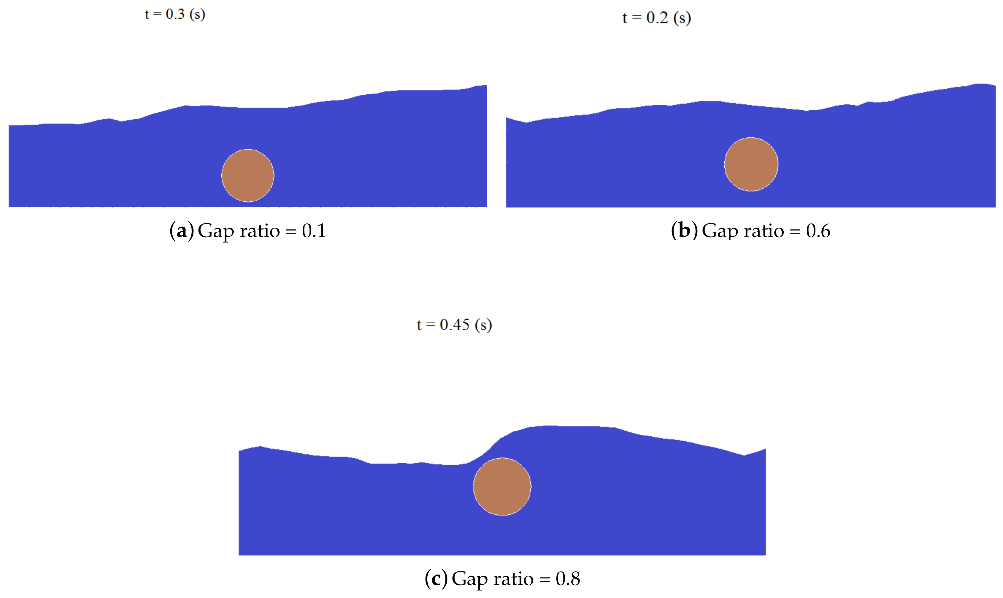
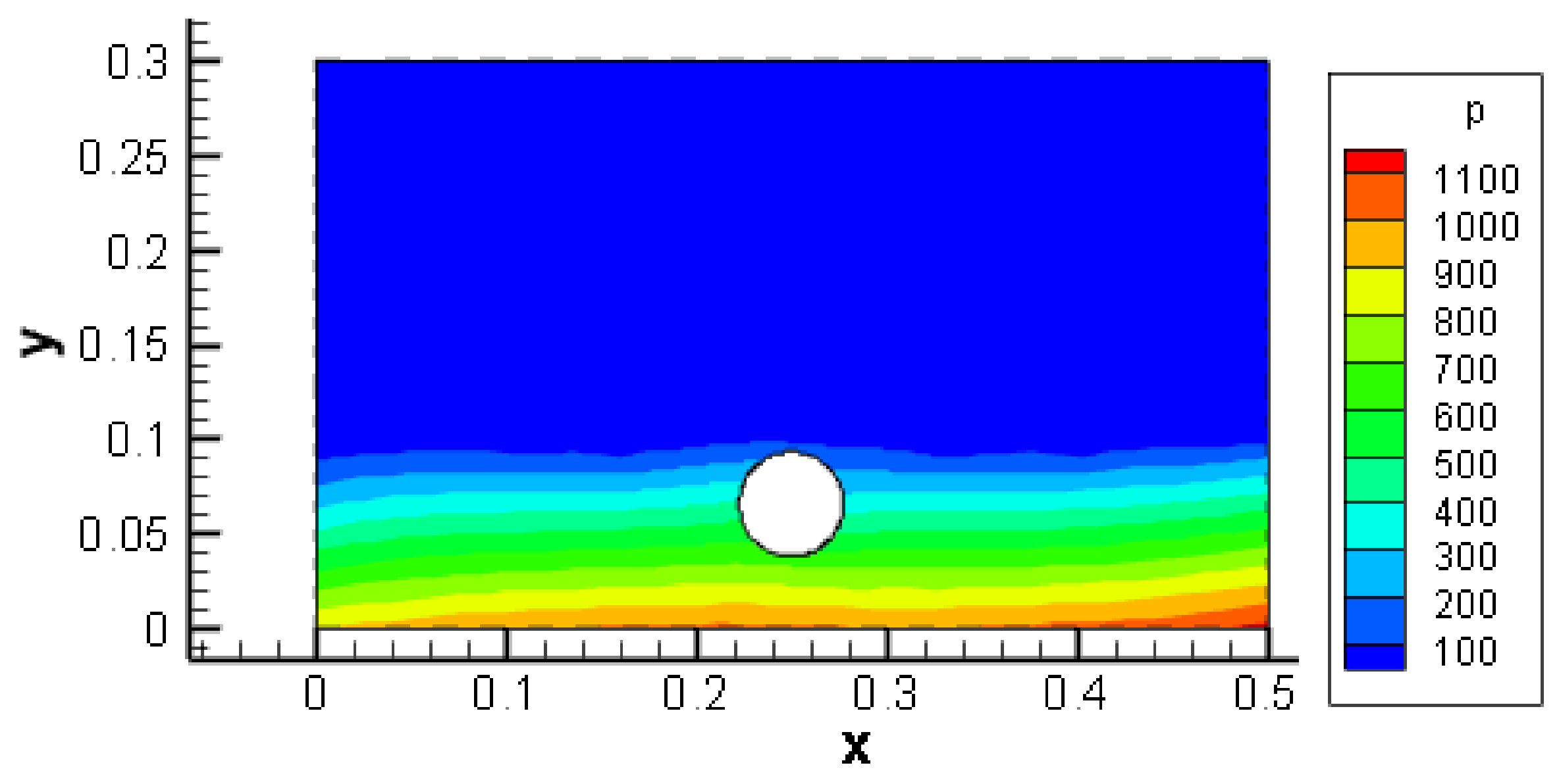
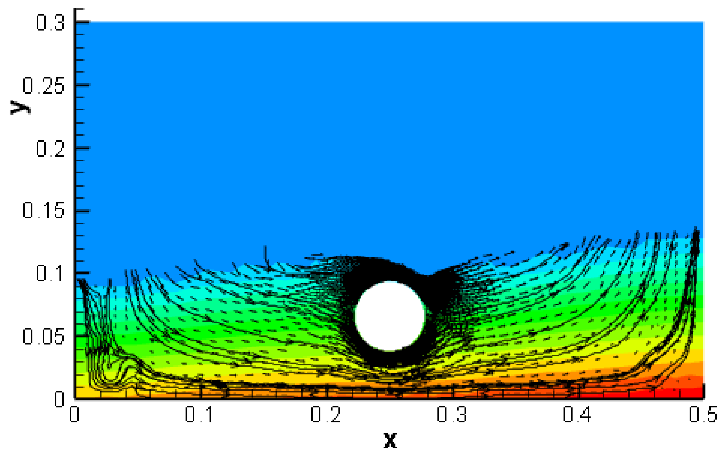
Numerical recreations are performed for three unique places of the ring perplex with reference to the free surface. Adequacy in controlling the free surface variety under a remotely forced horizontal excitation is attempted. Free surface elevation of the fluid at various distances from the side wall is presented in Figure 3. Figure 3a presented the fluid level at t = 0.3 s for Gap ratio equals to 0.1 which the free surface doesn’t affect properly by baffle. Figure 3b presented the fluid level at t = 0.45 s for Gap ratio equal to 0.6. Figure 3c presented the fluid level at t = 0.2 s for Gap ratio equal to 0.8 as shown in the approach of baffle to free surface causing higher wave breaking. Based on the analysis of Dodge et al. [23], which showed that the interface shape is the most important parameter, we started here with the effect of gap with the bottom wall. Consider a cylindrical baffle that used in the simulation as shown in Figure 4, with fill level = 37%. The liquid volumes in all cases are equal. Figure 4 shows the pressure distribution for filling level of 11 cm and 6.6 cm distance of 3.85 cm from the bottom at a time of 0.1 s, which illustrates the effect of initial acceleration on the curvature of interface. Fluid flow advection mainly happens between baffle and the bottom wall.

Pressure and velocity in liquid for filling level = 37% and $0.6\times h_f$ distance from bottom at $t=1\times \left(s\right)$ appear in Figure 5. Velocity near the cylinder in the fluid stage is higher than the other points. As is shown, the existence of the baffle causes fluid flow stratification. Due to the tuned liquid damper, the zone of fluid wet divider is bigger; accordingly, it sets aside more opportunity for the viscous effect to be exchanged to the bulk fluid.

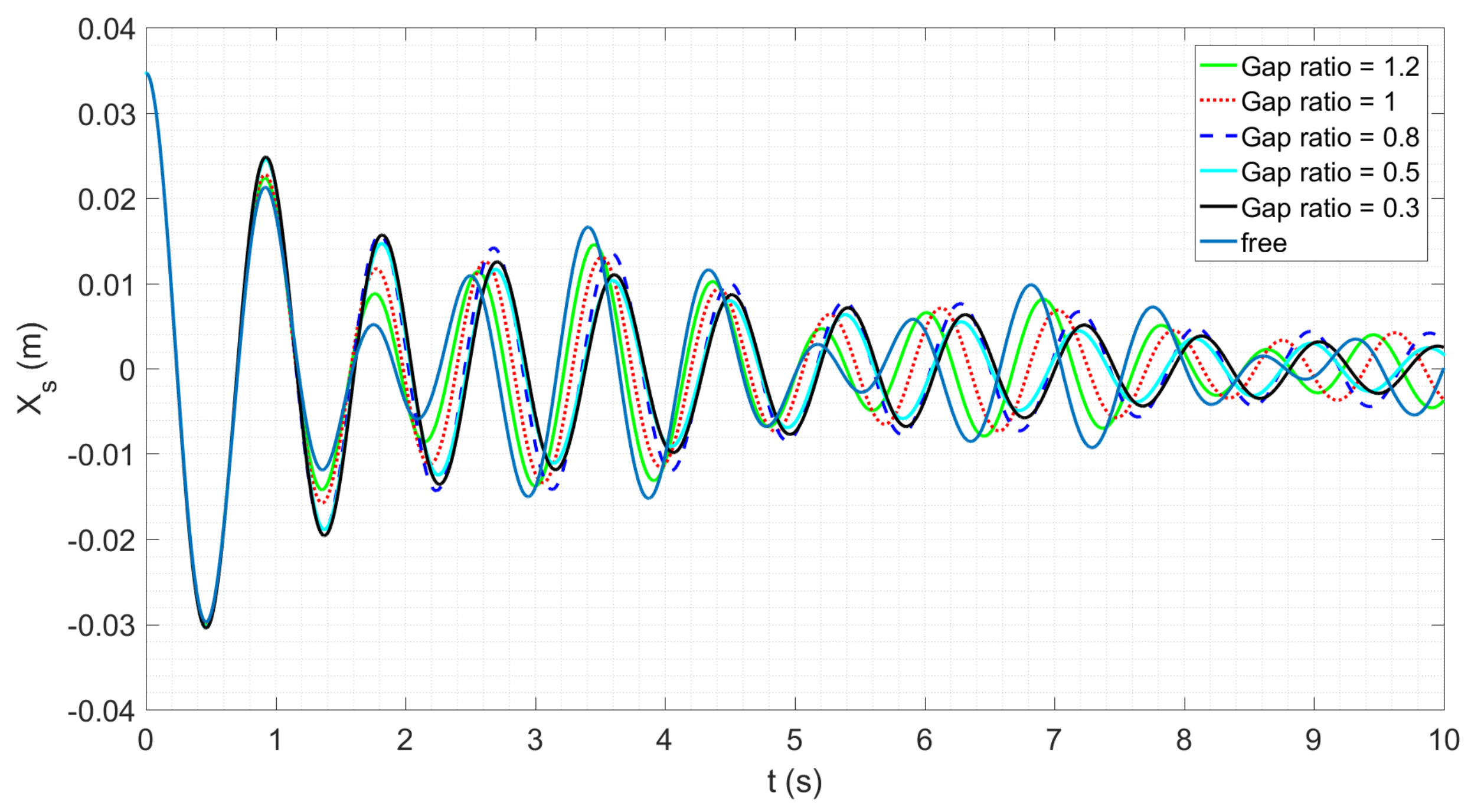
Figure 6 shows the structure position under different gap distances. As is shown, adding the baffle increases the tuned liquid system damping.

By using the tool of dimensional analysis, we can classify the regime of fluid–solid interactions. By defining a dimensional velocity by dividing $U_s$ by $U_f$, one can define the dimensional number. Reduced velocity number, $U_R$, is a dimensionless number that shows that the relative velocity of fluid to solid is defined as

$$U_R=\frac{sqrt(g\times h_f)}{x_0\times {\omega }_s},$$

(17)

where $h_f$ in this case stands for fluid height, g is the gravity coefficient, $x_0$ is the initial location of structure from static equilibrium point, and $w_s$ is the liquid angular velocity. As the baffle is considered as a rigid body, Mass number (relative density), Cauchy number (fluid pressure to Young modulus) will not affect the system, while the Reynolds number (viscosity effect around the cylinder) and Fraud number (gravity pressure effect) are important. The added mass is constant in all $U_R$, the added damping is $\propto U_R$, and the added stiffness is $\propto U_R^2$. As here the $T_f\approx T_s$ or $U_R\approx 1$, the fluid motion $\ddot{p}=-{\omega }_f^{2}p$ and solid motion $\ddot{x_s}=-{\omega }_s^2{x}_s$ are coupled via dynamic condition ${\rho }_f\times {(x_s\times {\omega }_s)}^2\times h_f\times W\approx k_s\times x_s$.

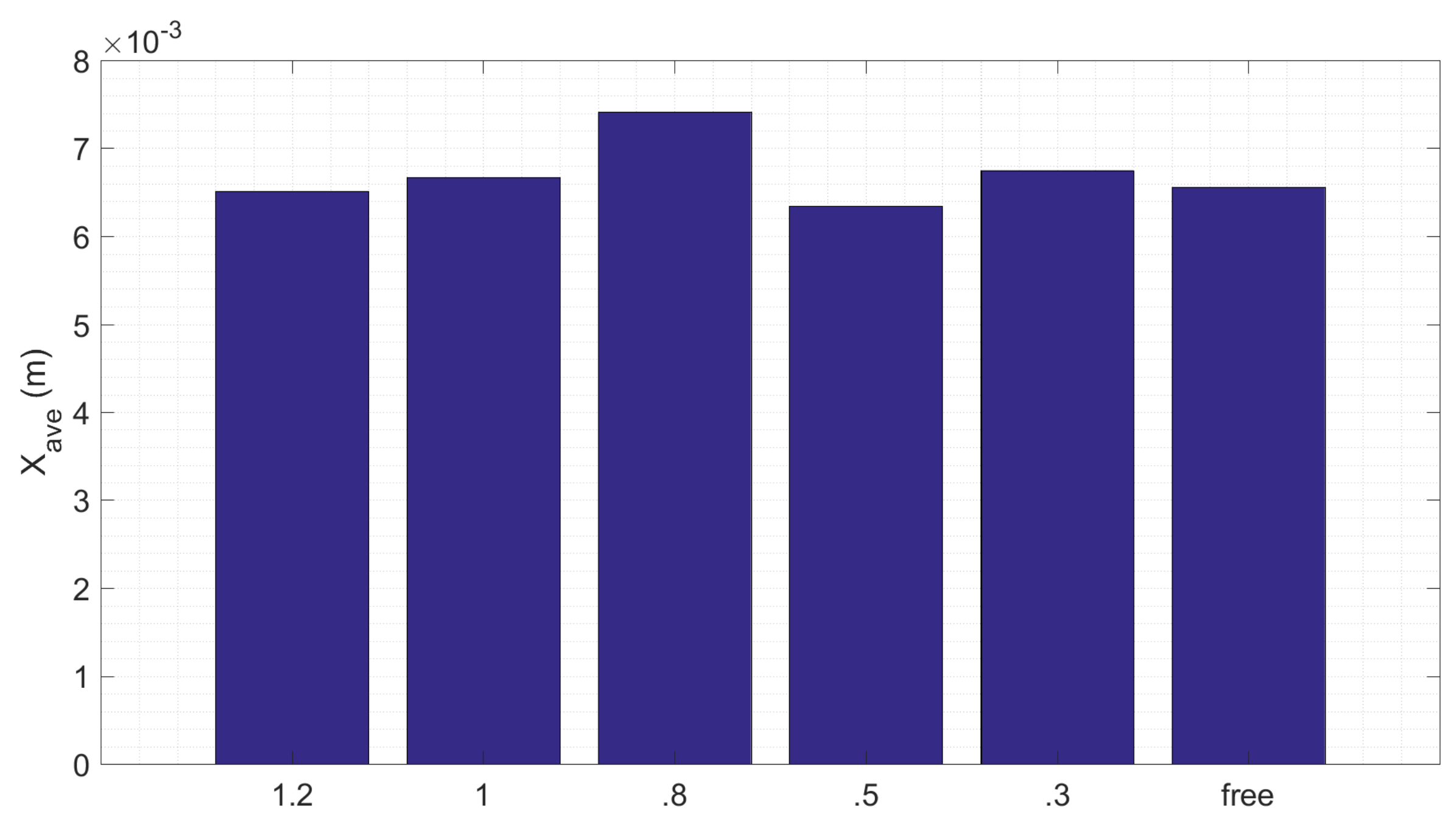
Average distortion versus gap distance ratios are shown in Figure 7. Although all the cases shown in Figure 6 have a lower value of $X_s$ than the free vibration of the structure, the total behavior is investigated in Figure 7. As is shown, the average of norm of structure position in case of $h_c=0.8h_f$ is higher than the free vibration of structure because of the transient overshoot of this case in the first period of vibration. In addition, the best cases happen in $h_c=0.5h_f$, which can be considered as the optimal location. When the baffle is at $h_c=0.5h_f$, the advection has a wide range, and the average magnitude of velocity is higher. Although the maximum displacement of the tank solid is different in these two configurations, the velocity field in the middle and bottom parts of the tank is similar.

3.3. Effect of Filling Level

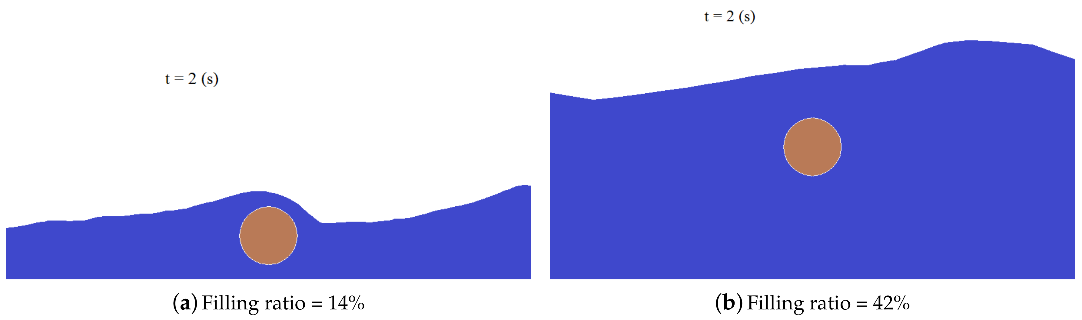
The effect of filling ratio is shown in Figure 8. The solid displacement versus fill level ought to have a pattern as the dashed line in the tank without a perplex. Normally, the increase of filling ratio helps increment the fluid frequency, advance dissipation and bring damping up in the tank. Furthermore, the sloshing motion apportioning model states that the dissipation from baffle to tank is comprised of three regions: the damping of the top breaking wave, the dissipation for exposing wave on the sides and the dissipation from the flow in the bottom of the cylinder. For the current situation, dissipation exchanged from the fluid wet boundary affects the adjacent fluid. Subsequently, the wet region near the baffle and thickness of the boundary layer of fluid close baffle, which compare to the capacity of all boundaries of the vessel that exchange momentum by fluid, impact dissipation incredibly. On account of the presence of cylindrical baffle near the surface, when fill level is near the wall of the cylinder, fluid will move up to the top boundary of the cylinder by surface wave; along these lines, dissipation exchanged to the fluid stage. In this manner, the increase in dissipation will be smaller in the event that it is working. Thus, we get a sharp decrease as fill level increases. The progress point is somewhat higher than 40%, which can submerge the base baffle in an ordinary system, at around 50%. For the current paper where the $D=\frac{h_f}{2}$ at the point when fill level is 18%, the fluid is enough to fill the space between the cylinder and the bottom wall, and fluid that filled later will show up at the center of the tank, an area that isn’t viable for blocking the fluid between two regions. In this way, for levels somewhat over 18%, interfaces are comparatively close dividers, as shown in Figure 9, so the damping ratio is increased. In addition, when fill level is low, 30% for instance, fluid predominantly exists under the cylinder base flow and isn’t sufficient to cover the divider between two zones. At the point when the fill level is over 70%, the gas momentum is huge in the upper segment over the cylinder; in this way, the impact of baffle is feeble. Consequently, the baffles can moderate momentum ascension for fill levels in the cylinder and the bottom, which is useful in light of the fact that the liquid in the rigid tank normally lessens from full to purge during the mission. Average distortion versus gap distance ratios is shown in Figure 8. Although all the cases shown in Figure 9 have lower values of $X_s$ than the free vibration of structure, the total behavior is investigated in Figure 8. Free surface elevation of the fluid at various filling levels is shown in Figure 10 for filling ratio of 14% in Figure 10a and for filling ratio of 42% in Figure 10b, respectively, for time equal to 2 sonds. The free surface is not smooth here as the wave breaking happens through the sloshing. As is shown, lower filling ratio causes higher wave breaking and thus lower displacement for the structure, as shown in Figure 9. In addition, the difference between 11 cm and 7 cm levels is sensitive to the forces in the vehicle.

3.4. Distance from the Side Wall

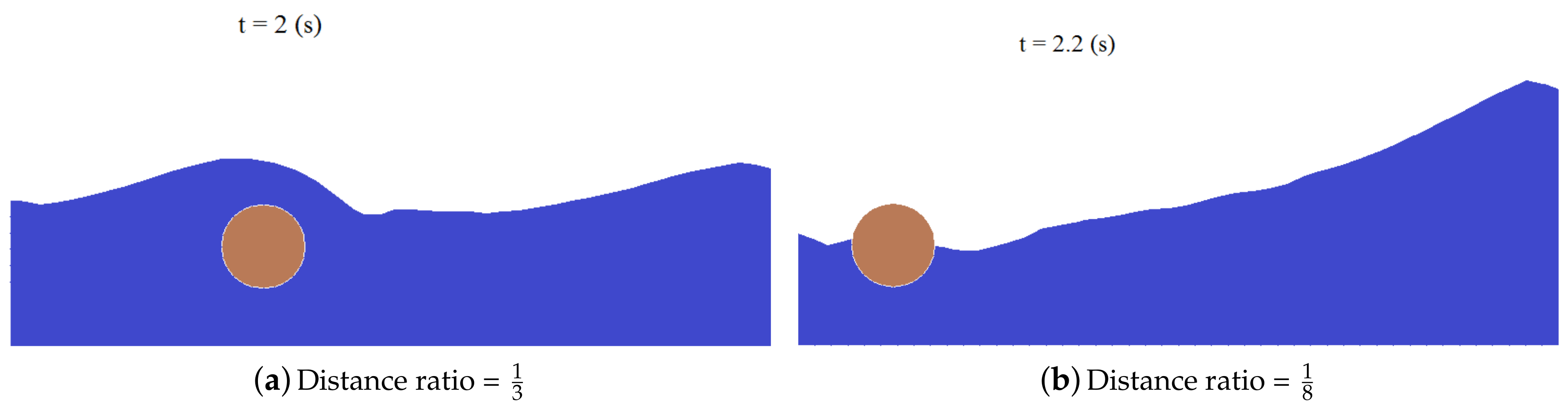
Control of slosh powers and free surface wave stature affected by horizontal excitation is absolutely alluring. Albeit a few dynamic and aloof techniques have been proposed in the open writing, utilizing inside puzzles is the most straightforward of every such arrangement. For a straightforward stockpiling tank, a position with reference to the free surface, width and thickness of the bewilder is a basic plan included. Simulations are performed for tanks with different baffle distances from the left wall in Figure 11. During the simulation, fluid interface climbs up to the edge of tanks at the beginning, then covers baffle as much as it can by surface tension, and then becomes damped for the rest of the simulation. The effect of distance from the side wall on liquid sloshing could be considerable when the tank is subjected to horizontal excitation. Both low and extensive separations between wall and baffle can moderate the fluid motion, and the decrease of solid motion ascending against distance is shown in Figure 11 with fill level of 50%. This is on account of the fact that, at zero distance, which isn’t exceptional in moderating sloshing, the liquid changes dramatically, and thus the fluid vortexes as well. According to the normal VOF technique, fluid volumes with close interfaces have decimal qualities. The adjustment in fluid volumes results in development of an interface. During the damping procedure in the first initial second, interface in the baffled tank encounters quick acceleration. Be that as it may, as separation builds, the vacillation is essentially facilitated. We can see little changes in the distance ratio = $\frac{1}{3}$ case; however, for distance ratio = $\frac{1}{8}$, the fluid volume is just about consistent near 1.

As distance increases, the contribution of reducing sloshing waves changes from diffusion to breaking waves as the wet area increases. However, in cases of distance ratios $\frac{1}{8}$ and $\frac{1}{3}$, the sloshing phenomenon is weakened by baffles, but the liquid near the wall is too thin to weaken the wave momentum effectively as the liquid is fluctuating.

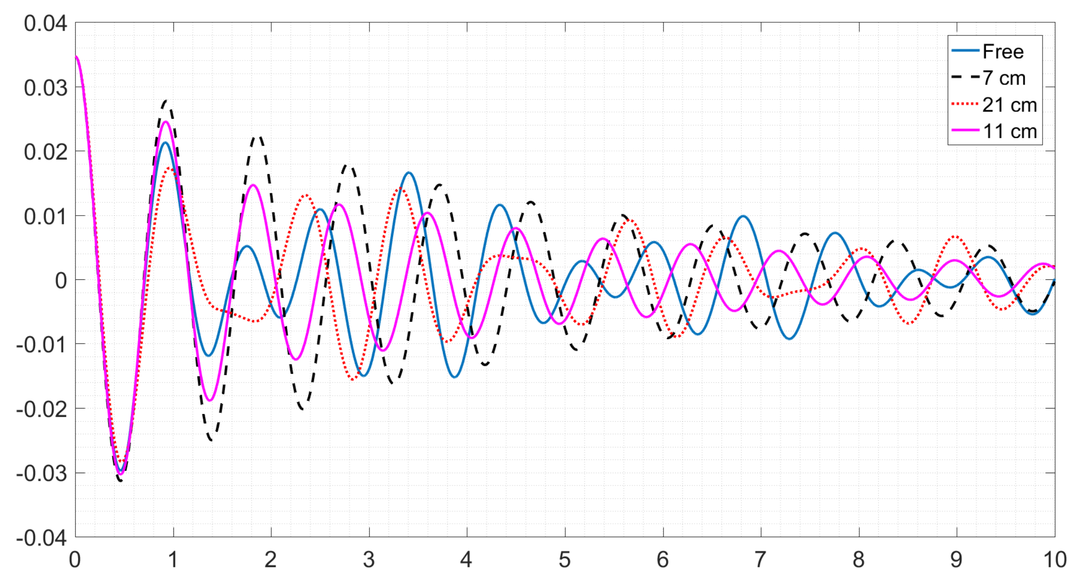
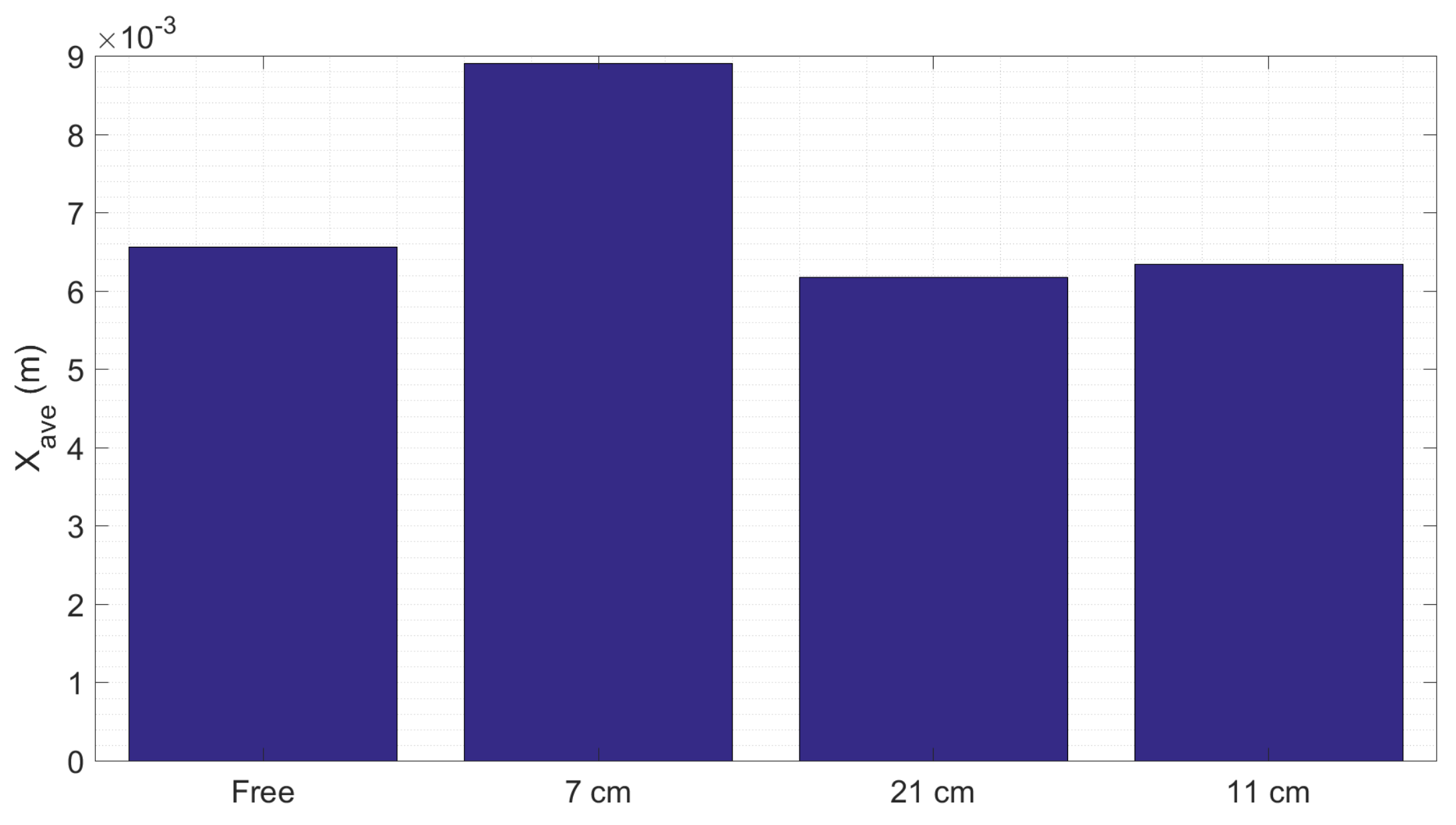
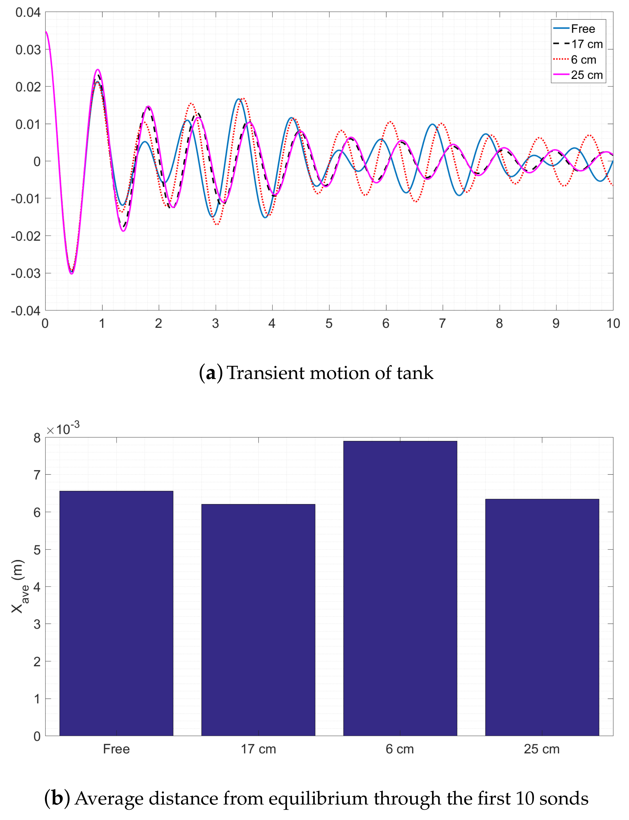
The comparison of solid distribution and velocity field between distance ratio is $\frac{1}{8}$ and $\frac{1}{3}$ is shown in Figure 11. Thus, we get the profiles as shown in Figure 12. As is shown in Figure 12a, a periodical force is applied to the tank wall. The differences in 17 cm and 21 cm distances are quite small such that one that cannot be correctly predicted will cause the failure of the mission. As is shown in Figure 12b, a large distance from the wall is preferred.

4. Conclusions

In this paper, a parameter study on the optimization of baffle on vibration suppression of a partially filled rectangular rigid tank coupled by structure has been performed. The coupled system is released from an initial displacement without a velocity. Navier–Stokes governing equations coupled by the equation of volume of fluid and a single degree of freedom structure are solved. As is shown, higher performance can be easily achieved by considering effective parameters. Specific findings from the present numerical simulations can be outlined as follows:

• The near wall zone plays an important role in dampening the fluid momentum in the tank.
• The baffle located close to the free surface is effective in control of surface fluctuations, as well as concomitant force and pressure.
• The filling ratio affects the wet wall fraction and sloshing frequency.
• The existence of distances from the wall influences the wet wall area (surface tension effect), and liquid can climb up to the baffle if the baffle is near the surface.
• As the sloshing in the tank is steady, baffles can do little with wave breaking and have no influence on the behavior of liquid.
• The liquid thickness has more importance in slosh damping than wet area.
• The parameter studied here based on importance are the distances, filling ratio, and gaps of the baffle
• Based on a detailed study of transient structure motion coupled with sloshing dynamics, and by optimizing the parameters of baffle, optimal baffle location was achieved.

References

- Nasiri, H.; Abdollahzadeh Jamalabadi, M.Y.; Sadeghi, R.; Nguyen, T.K.; Safdari Shadloo, M. A smoothed particle hydrodynamics approach for numerical simulation ofnano-fluid flows: Application to forced convection heat transfer over a horizontal cylinder. J. Therm. Anal. Calorim. 2018, 1–19. [Google Scholar] [CrossRef]
- Jamalabadi, M.Y.A.; Daqiqshirazi, M.; Nasiri, H.; Safaei, M.R.; Nguyen, T.K. Modeling and analysis ofbiomagnetic blood Carreau fluid flow through astenosis artery with magnetic heat transfer: A transient study. PLoS ONE 2018, 484, e0192138. [Google Scholar]
- Abdollahzadeh Jamalabadi, M.Y.; Safaei, M.R.; Alrashed, A.A.A.A.; Nguyen, T.K.; Filho, E.P.B. Entropy generation in thermalradiative loading of structures with distinct heaters. Entropy 2017, 19, 506. [Google Scholar] [CrossRef]
- Abdollahzadeh Jamalabadi, M.Y.; Bidokhti, A.A.A.; Rah, H.K.; Vaezi, S.; Hooshmand, P. Numerical investigation of oxygenated anddeoxygenated blood flow through a taperedstenosed arteries in magnetic field. PLoS ONE 2016, 12, e0167393. [Google Scholar]
- Abdollahzadeh Jamalabadi, M.Y. Microrobots propulsion system design for drug delivery. J. Chem. Pharm. Res. 2016, 8, 448–496. [Google Scholar]
- Abdollahzadeh Jamalabadi, M.Y.; Keikha, A.J. Fluid–solid interaction modeling ofcerebrospinal fluid absorption inarachnoid villi. J. Chem. Pharm. Res. 2016, 8, 428–442. [Google Scholar]
- Sadeghi, R.; Shadloo, M.S.; Hopp-Hirschler, M.; Hadjadj, A.; Nieken, U. Three-dimensional lattice Boltzmann simulations of high density ratio two-phase flows in porous media. Comput. Math. Appl. 2018, 75, 2445–2465. [Google Scholar] [CrossRef]
- Shadloo, M.S.; Weiss, R.; Yildiz, M.; Dalrymple, R.A. Numerical Simulations of the Breaking and Non-breaking Long Waves. Int. J. Offshore Polar Eng. 2015, 25, 1–7. [Google Scholar]
- Shadloo, M.S.; Rahmat, A.; Yildiz, M. A Smoothed Particle Hydrodynamics Study on theElectrohydrodynamic Deformation of a Droplet Suspended in a Neutrally Buoyant Newtonian Fluid. Comput. Mech. 2013, 52, 693–707. [Google Scholar] [CrossRef]
- Sadeghi, R.; Shadloo, M.S. Three-dimensional Numerical Investigation of Film Boiling by Lattice Boltzmann Method. Numer. Heat Transf. Part A Appl. 2017, 71, 374–385. [Google Scholar] [CrossRef]
- Sadeghi, R.; Shadloo, M.S.; Hooman, K. Numerical Investigation of Natural Convection Film Boiling Around Elliptical Tubes. Numer. Heat Transf. Part A Appl. 2016, 70, 707–722. [Google Scholar] [CrossRef]
- Fatehi, R.; Shadloo, M.S.; Manzari, M.T. Numerical Investigation of Two-Phase Secondary Kelvin-Helmholtz Instability. J. Mech. Eng. Sci. 2014, 228, 1913–1924. [Google Scholar] [CrossRef]
- Shadloo, M.S.; Yildiz, M. Numericalmodelling of Kelvin-Helmholtz Instability Using Smoothed Particle Hydrodynamics Method. Int. J. Numer. Methods Eng. 2011, 87, 988–1006. [Google Scholar] [CrossRef]
- Shadloo, M.S.; Oger, G.; le Touze, D. Smoothed Particle Hydrodynamics Method for Fluid Flows, Towards Industrial Applications: Motivations, Current state, and Challenges. Comput. Fluids 2016, 136, 11–34. [Google Scholar] [CrossRef]
- Rahmat, A.; Tofighi, N.; Shadloo, M.S.; Yildiz, M. Numerical Simulation of Wall Bounded and Electrically Excited Rayleigh Taylor Instability Using Incompressible Smoothed Particle Hydrodynamics. Colloids Surf. A 2014, 460, 60–70. [Google Scholar] [CrossRef]
- Lebon, B.; Nguyen, M.Q.; Peixinho, J.; Shadloo, M.S.; Hadjadj, A. A new mechanism for the periodic bursting of therecirculation region of the flow through a sudden expansion in a circular pipe. Phys. Fluids 2018, 30, 031701. [Google Scholar] [CrossRef]
- Nguyen, M.Q.; Lebon, B.; Shadloo, M.S.; Peixinho, J.; Hadjadj, A. New features of transition to turbulence in a sudden expansion pipe flow. arXiv, 1807; arXiv:1807.10665. [Google Scholar]
- Sumner, I.; Lacovic, R.; Stofan, A. Experimental Investigation of Liquid Sloshing in a Scale-Model Centaur Liquid-Hydrogen Tank; National Aeronautics and Space Administration: Washington, DC, USA, 1966. [Google Scholar]
- Panzarella, C.; Kassemi, M. On the validity of purely thermodynamic descriptions of two-phase cryogenic fluid storage. J. FluidMech. 2003, 484, 41–68. [Google Scholar] [CrossRef]
- Yoon, S.-H.; Park, K.-J. Effect of baffles on sloshing mitigation in liquid storage tanks. Adv. Sci. Technol. Lett. 2015, 108, 1–5. [Google Scholar]
- Hasheminejad, S.; Mohammadi, M.M. Effect of anti-slosh baffles on free liquid oscillations in partially filled horizontal circular tanks. Ocean Eng. 2011, 38, 49–62. [Google Scholar] [CrossRef]
- Hasheminejad, S.M.; Aghabeigi, M. Sloshing characteristics in half-full horizontal elliptical tanks with vertical baffles. Appl. Math. Model. 2012, 36, 57–71. [Google Scholar] [CrossRef]
- Dodge, F.T. The New “Dynamic Behavior of Liquids in Moving Containers”; Southwest Research Instution: San Antonio, TX, USA, 2000. [Google Scholar]
- Kannape, M.; Przekwa, A.; Singhal, A.; Costes, N. Liquid oxygen sloshing in space shuttle external tank. In Proceedings of the 23rd Joint Propulsion Conference, San Diego, CA, USA, 24–27 June 1987; p. 2019. [Google Scholar]
- Dogde, F. The New dynamic Behavior of Liquids in Moving Containers; Southwest Reserach Inst.: San Antonio, TX, USA, 2000. [Google Scholar]
- Adam, P.; Leachman, J. Design of areconfigurable liquid hydrogen fuel tank for use in the genii unmanned aerial vehicle. AIP Conf. Proc. 2014, 1573, 1299–1304. [Google Scholar]
- Strauch, H.; Luig, K.; Bennani, S. Model based design environment for launcher upper stagegnc development. In Proceedings of the Workshop on Simulation for European Space Programmes SESP, Noordwijk, The Netherlands, 6–8 November 2014. [Google Scholar]
- Behruzi, P.; Konopka, M.; de Rose, F.; Schwartz, G. Cryogenic slosh modeling inlng ship tanks and spacecrafts. In Proceedings of the Twenty-Fourth International Ocean and Polar Engineering Conference, Busan, Korea, 15–20 June 2014. [Google Scholar]
- Grayson, G.; Lopez, A.; Chandler, F.; Hastings, L.; Tucker, S. Cryogenic tank modeling for thesaturn as-203 experiment. In Proceedings of the 42nd AIAA/ASME/SAE/ASEE Joint Propulsion Conference & Exhibit, Sacramento, CA, USA, 9–12 July 2006; p. 5258. [Google Scholar]
- Seo, M.; Jeong, S. Analysis of self-pressurization phenomenon of cryogenic fluid storage tank with thermal diffusion model. Cryogenics 2010, 50, 549–555. [Google Scholar] [CrossRef]
- Ma, Y.; Li, Y.; Zhu, K.; Wang, Y.; Wang, L.; Tan, H. Investigation on no-vent filling process of liquid hydrogen tank undermicrogravity condition. Int. J. Hydrogen Energy 2017, 42, 8264–8277. [Google Scholar] [CrossRef]
- Frandsen, J.B. Sloshing motions in excited tanks. J. Comput. Phys. 2004, 196, 53–87. [Google Scholar] [CrossRef]
- Chintalapati, S.; Kirk, D. Parametric study of a propellant tank slosh baffle. In Proceedings of the 44th AIAA/ASME/SAE/ASEE Joint Propulsion Conference & Exhibit, Hartford, CT, USA, 21–23 July 2008; p. 4750. [Google Scholar]
- Hirt, C.; Nichols, B.D. Volume of fluid (vof) method for the dynamics of free boundaries. J. Comput. Phys. 1981, 39, 201–225. [Google Scholar] [CrossRef]
- Nakayama, T.; Washizu, K. Boundary element analysis of nonlinear sloshing problems. In Developments in Boundary Element Method-3; Elsevier Applied Science Publishers: New York, NY, USA, 1984. [Google Scholar]
- Fries, N.; Behruzi, P.; Arndt, T.; Winter, M.; Netter, G.; Renner, U. Modelling of fluid motion in spacecraft propellant tanks-sloshing. In Proceedings of the Space Propulsion Conference, Bordedaux, France, 7–10 May 2012. [Google Scholar]
- Behruzi, P.; Rose, F.; Cirillo, F. Coupling sloshing, gnc and rigid body motions during ballistic flight phases. In Proceedings of the AIAA Joint Propulsion Conference (AIAA 2016-4586), Salt Lake City, UT, USA, 25–27 July 2016. [Google Scholar]
- Gerstmann, J.; Konopka, M. Cryo-laboratory for test and development of propellant management technologies. In Proceedings of the 2nd International Spacecraft Propulsion Conference (SP2015_3124996), Kyoto, Japan, 14–18 September 2015. [Google Scholar]
- Kartuzova, O.; Kassemi, M. Modeling interfacial turbulent heat transfer duringventless pressurization of a large scale cryogenic storage tank inmicrogravity. In Proceedings of the 47 th AIAA/ASME/SAE/ASEE Joint Propulsion Conference & Exhibit, San Diego, CA, USA, 31 July–3 August 2011; p. 6037. [Google Scholar]
- Kurul, N.; Podowski, M.Z. Multidimensional effects in forced convectionsubcooled boiling. In Proceedings of the Ninth International Heat Transfer Conference, Jerusalem, Israel, 19–24 August 1990; Hemisphere Publishing: New York, NY, USA, 1990; Volume 2, pp. 19–24. [Google Scholar]
- Apkarian, P.; Dao, N.; Noll, D. Parametric robust structured control design. IEEE Trans. Autom. Control 2015, 60, 1857–1869. [Google Scholar] [CrossRef]
- Konopka, M.; De Rose, F.; Arndt, T.; Gerstmann, J. Large-scale tank active sloshing damping simulation and experiment. In Proceedings of the 3rd International Spacecraft Propulsion Conference (SP2016_3124606), Rome, Italy, 2–6 May 2016. [Google Scholar]
- Zhou, K.; Doyle, J. Essentials of Robust Control; Prentice-Hall: Upper Saddle River, NJ, USA, 1998. [Google Scholar]
- Hecker, S.; Varga, A. Generalized lft-based representation of parametric uncertain models. Eur. J. Control 2004, 10, 326–337. [Google Scholar] [CrossRef]
- Falcoz, A.; Pittet, C.; Bennani, S.; Guignard, A.; Bayart, C.; Frapard, B. Systematic design methods of robust and structured controllers for satellites. CEAS Space J. 2015, 7, 319–334. [Google Scholar] [CrossRef]
- Achenbach, E. Influence of Surface Roughness on the Cross-Flow Around a Circular Cylinder. J. Fluid Mech. 1971, 46, 321–335. [Google Scholar] [CrossRef]
- Basara, B.; Krajnović, S.; Girimaji, S.; Pavlovic, Z. Near-Wall Formulation of the Partially Averaged Navier–Stokes Turbulence Model. Am. Inst. Aeronaut. Astronaut. J. 2011, 49, 2627–2636. [Google Scholar] [CrossRef]
- Bloor, M.S. The Transition to Turbulence in the Wake of a Circular Cylinder. J. Fluid Mech. 1964, 19, 290–304. [Google Scholar] [CrossRef]
- Chaouat, B.; Schiestel, R. A New Partially Integrated Transport Model forSubgrid-Scale Stresses and Dissipation Rate for Turbulent Developing Flows. Phys. Fluids 2005, 17, 065106. [Google Scholar] [CrossRef]
- Fage, A.; Warsap, J.H. The Effects of Turbulence and Surface Roughness on the Drag of a Circular Cylinder. Aeronaut. Res. Comm. 1929, 39, 335–342. [Google Scholar]
- Fasel, H.F.; Seidel, J.; Wernz, S. A Methodology for Simulations for Complex Turbulent Flows. J. Fluids Eng. 2002, 124, 933–942. [Google Scholar] [CrossRef]
- Gatski, T.B.; Speziale, C.G. On Explicit Algebraic Stress Models for Complex Turbulent Flows. J. Fluid Mech. 1993, 254, 59–78. [Google Scholar] [CrossRef]
- Gerich, D.; Eckelmann, H. Influence of End Plates and Free Ends on the Shedding Frequency of Circular Cylinders. J. Fluid Mech. 1982, 122, 109–121. [Google Scholar] [CrossRef]
- Germano, M. Turbulence: The Filtering Approach. J. Fluid Mech. 1992, 238, 325–336. [Google Scholar] [CrossRef]
- Girimaji, S.S. Fully Explicit and Self-Consistent Algebraic Reynolds Stress Model. Theor. Comput. Fluid Dyn. 1996, 8, 387–402. [Google Scholar] [CrossRef]
- Reyes, D.A.; Cooper, J.M.; Girimaji, S.S. Characterizing Velocity Fluctuations in Partially Resolved Turbulence Simulations. Phys. Fluids 2014, 26, 085106. [Google Scholar] [CrossRef]
- Girimaji, S.S. Pressure-Strain Correlation Modelling of Complex Turbulent Flows. J. Fluid Mech. 2000, 422, 91–123. [Google Scholar] [CrossRef]
- Girimaji, S.S. Lower-Dimensional Manifold (Algebraic) Representation of Reynolds Stress Closure Equations. Theor. Comput. Fluid Dyn. 2001, 14, 259–281. [Google Scholar] [CrossRef]
- Girimaji, S. Partially-Averaged Navier–Stokes Model for Turbulence: A Reynolds-AveragedNavier–Stokes to Direct Numerical Simulation Bridging Method. J. Appl. Mech. 2005, 73, 413–421. [Google Scholar] [CrossRef]
- Girimaji, S.S.; Abdol-Hamid, K.S. Partially-Averaged Navier Stokes Model for Turbulence: Implementation and Validation. In Proceedings of the 43rd American Institute of Aeronautics and Astronautics (AIAA) Aerospace Sciences Meeting and Exhibit, Reno, NV, USA, 10–13 January 2005. [Google Scholar]
- Girimaji, S.S.; Jeong, E.; Srinivasan, R. Partially Averaged Navier–Stokes Method for Turbulence: Fixed Point Analysis and Comparison With Unsteady Partially Averaged Navier–Stokes. J. Appl. Mech. 2005, 73, 422–429. [Google Scholar] [CrossRef]
- Güven, O.; Farrel, C.; Patel, V.C. Surface-Roughness Effects on the Mean Flow Past Circular Cylinder. J. Fluid Mech. 1980, 98, 673–701. [Google Scholar] [CrossRef]
- Huang, Y.-N.; Rajagopal, K.R. On a Generalized Nonlinear k-ϵ Model for Turbulence that Models Relaxation Effects. Theor. Comput. Fluid Dyn. 1996, 8, 275–288. [Google Scholar]
- Hussain, A.K.M.F.; Reynolds, W.C. The Mechanics of an Organized Wave in Turbulent Shear Flow. J. Fluid Mech. 1970, 41, 241–258. [Google Scholar] [CrossRef]
- Kok, J.C. A Stochastic Backscatter Model for Grey-Area Mitigation in Detached Eddy Simulations. Flow Turbul. Combust. 2017, 99, 119–150. [Google Scholar] [CrossRef]
- Pereira, F.S.; Vaz, G.; Eça, L. An Assessment of Scale-Resolving Simulation Models for the Flow Around a Circular Cylinder. Turbul. Heat Mass Transf. (THMT) 2015, 8. [Google Scholar]
- Kok, J.C.; Dol, H.S.; Oskam, B.; der Ven, H.V. Extra-Large Eddy Simulation of Massively Separated Flows. In Proceedings of the 42nd American Institute of Aeronautics and Astronautics (AIAA) Aerospace Sciences Meeting and Exhibit, Reno, NV, USA, 5–8 January 2004. [Google Scholar]
- Muschinski, A. A Similarity Theory of Locally Homogeneous and Isotropic Turbulence Generated by aSmagorinsky-Type LES. J. Fluid Mech. 1996, 325, 239–260. [Google Scholar] [CrossRef]
- Mishra, A.A.; Girimaji, S.S. Intercomponent Energy Transfer inIncompressible Homogeneous Turbulence: Multi-Point Physics and Amenability to One-Point Closures. J. Fluid Mech. 2013, 731, 639–681. [Google Scholar] [CrossRef]
- Koopmann, G.H. The Vortex Wake of Vibrating Cylinders at Low Reynolds Numbers. J. Fluid Mech. 1967, 28, 501–512. [Google Scholar] [CrossRef]
- Lehmkuhl, O.; Rodriguez, I.; Borrel, R.; Oliva, A. Low-Frequency Unsteadiness in the Vortex Formation of a Circular Cylinder. Phys. Fluids 2013, 25, 085109. [Google Scholar] [CrossRef] [Green Version]
- Lakshmipathy, S.; Girimaji, S.S. Partially-AveragedNavier–Stokes Method for Turbulent Flows: k-ω Model Implementation. In Proceedings of the 44th American Institute of Aeronautics and Astronautics (AIAA) Aerospace Sciences Meeting and Exhibit, Reno, NV, USA, 9–12 January 2006. [Google Scholar]
- Schiestel, R. Multiple-Time-Scale Modeling of Turbulent Flows in One-Point Closures. Phys. Fluids 1987, 30, 722–731. [Google Scholar] [CrossRef]
- Wilcox, D.C. Reassessment of the Scale-Determining Equation for Advanced Turbulence Models. Am. Inst. Aeronaut. Astronaut. J. 1988, 26, 1299–1310. [Google Scholar] [CrossRef]
- Schiestel, R.; Dejoan, A. Towards a New Partially Integrated Transport Model for Coarse Grid and Unsteady Flow Simulation. Theor. Comput. Fluid Dyn. 2005, 18, 443–468. [Google Scholar] [CrossRef]
- Pope, S.B. A More General Effective-Viscosity Hypothesis. J. Fluid Mech. 1975, 72, 331–340. [Google Scholar] [CrossRef]
- Shur, M.L.; Spalart, P.R.; Strelets, M.Kh.; Travin, A.K. A HybridRANS-LES Approach with Delayed-DES and Wall-Modelled LES Capabilities. Int. J. Heat Fluid Flow 2008, 29, 1639–1649. [Google Scholar] [CrossRef]
- Spalart, P.R.; Jou, W.-H.; Strelets, M.; Allmaras, S. Comments on the Feasibility of LES for Wings and on the HybridRANS/LES Approach. In Proceedings of the 1st Air Force Office of Scientific Research (AFOSR) International Conference onDNS/LES-Advances inDNS/LES, Ruston, LA, USA, 4–8 August 1997. [Google Scholar]
- Speziale, C. Computing Non-Equilibrium Turbulent Flow with Time-Dependent RANS and VLES. In Proceedings of the 15th International Conference on Numerical Methods in Fluid Dynamics, Monterey, CA, USA, 24–28 June 1996. [Google Scholar]
- Mishra, A.A.; Girimaji, S.S. Pressure-Strain Correlation Modeling: Towards Achieving Consistency with Rapid Distortion Theory. Flow Turbul. Combust. 2010, 85, 593–619. [Google Scholar] [CrossRef]
- Mishra, A.A.; Girimaji, S.S. Toward Approximating Non-Local Dynamics in Single-Point Pressure-Strain Correlation Closures. J. Fluid Mech. 2017, 811, 168–188. [Google Scholar] [CrossRef]
- Speziale, C.G.; Sarkar, S.; Gatski, T.B. Modelling the Pressure Strain-Rate Correlation of Turbulence: An Invariant Dynamical Systems Approach. J. Fluid Mech. 1991, 227, 245–272. [Google Scholar] [CrossRef]
- Menter, F.R.; Kuntz, M.; Langtry, R. Ten Years of Industrial Experience with the SST Turbulence Model. In Turbulence, Heat and Mass Transfer, 4th ed.; Hanjalić, K., Nagano, Y., Tummers, M., Eds.; Begell House, Inc.: Antalya, Turkey, 2003. [Google Scholar]
- Launder, B.E.; Reece, G.J.; Rodi, W. Progress in the Development of a Reynolds-Stress Turbulence Closure. J. Fluid Mech. 1975, 68, 537–566. [Google Scholar] [CrossRef]
- Rodi, W. A New Algebraic Relation for Calculating the Reynolds Stresses. Z. Angew. Math. Mech. (ZAMM) 1976, 56, 219–221. [Google Scholar]
- Lin, J.-C.; Vorobieff, P.; Rockwell, D. Three-Dimensional Patterns ofStreamwise Vorticity in the Near-Wake of a Cylinder. J. Fluids Struct. 1995, 9, 231–234. [Google Scholar] [CrossRef]
- Prasad, A.; Williamson, C.H.K. Three-Dimensional Effects in Turbulent Bluff-Body Wake. J. Fluid Mech. 1997, 343, 235–265. [Google Scholar] [CrossRef]
- Mansy, H.; Yang, P.-M.; Williams, D.R. Quantitative Measurements of Three-Dimensional Structures in the Wake of a Circular Cylinder. J. Fluid Mech. 1994, 270, 277–296. [Google Scholar] [CrossRef]
- Roshko, A. On the Development of Turbulent Wake from Vortex Streets; Tech. Rep. 1191; National Advisory Committee for Aeronautics: Washington, DC, USA, 1954. [Google Scholar]
- Sadeh, W.Z.; Saharon, D.B. Turbulence Effect on Crossflow Around a Circular Cylinder at Subcritical Reynolds Numbers; NASA Contractor Report 3622; National Aeronautics and Space Administration (NASA): Washington, DC, USA, 1982. [Google Scholar]
- West, G.S.; Apelt, C.J. The Effects of Tunnel Blockage and Aspect Ratio on the Mean Flow Past a Circular Cylinder with Reynolds Numbers Between 104 and105. J. Fluid Mech. 1982, 114, 361–377. [Google Scholar] [CrossRef]
- Norberg, C. An Experimental Investigation of the Flow Around a Circular Cylinder: Influence of Aspect Ratio. J. Fluid Mech. 1994, 258, 287–319. [Google Scholar] [CrossRef]
- Szepessy, S.; Bearman, P.W. Aspect Ratio and End Plate Effects on Vortex Shedding From a Circular Cylinder. J. Fluid Mech. 1992, 234, 191–217. [Google Scholar] [CrossRef]
- Norberg, C. LDV-Measurements in the Near Wake of a Circular Cylinder. Advances in Understanding of Bluff Body Wakes and Vortex-Induced Vibration; Washington, DC, USA, 1998. Available online: http://www.ht.energy.lth.se/fileadmin/ht/Norberg-FEDSM98-5202.pdf (accessed on 9 October 2018).
- Norberg, C. Pressure Distributions around a Circular Cylinder in Cross-Flow. In Proceedings of the Symposium on Bluff Body Wakes and Vortex-Induced Vibrations (BBVIV3), Port Arthur, Australia, 17–20 December 2002. [Google Scholar]
- Norberg, C. Fluctuating Lift on a Circular Cylinder: Review and New Measurements. J. Fluids Struct. 2003, 17, 59–96. [Google Scholar] [CrossRef]
- Norberg, C.; Sundén, B. Turbulence and Reynolds Number Effects on the Flow and Fluid Forces on a Single Cylinder in Cross Flow. J. Fluids Struct. 1987, 1, 337–357. [Google Scholar] [CrossRef]
- Parnaudeau, P.; Carlier, J.; Heitz, D.; Lamballais, E. Experimental and Numerical Studies of the Flow over a Circular Cylinder at Reynolds Number 3900. Phys. Fluids 2008, 20, 085101. [Google Scholar] [CrossRef]
- Pereira, F.S.; Vaz, G.; Eça, L.; Girimaji, S.S. Simulation of the Flow Around a Circular Cylinder at Re = 3900 with Partially-Averaged Navier–Stokes Equations. Int. J. Heat Fluid Flow 2017, 69, 234–246. [Google Scholar] [CrossRef]
- Prasad, A.; Williamson, C.H.K. The Instability of the Shear Layer Separating from a Bluff Body. J. Fluid Mech. 1997, 333, 375–402. [Google Scholar] [CrossRef]
- Unal, M.F.; Rockwell, D. On Vortex Shedding from a Cylinder. Part 1. The Initial Instability. J. Fluid Mech. 1988, 190, 419–512. [Google Scholar] [CrossRef]
- Rajagopalan, S.; Antonia, R.A. Flow Around a Circular Cylinder-Structure of the Near Wake Shear Layer. Exp. Fluids 2005, 38, 393–402. [Google Scholar] [CrossRef]
- Williamson, C.H.K. Vortex Dynamics in the Cylinder Wake. Annu. Rev. Fluid Mech. 1996, 28, 477–539. [Google Scholar] [CrossRef]
- Zdravkovich, M.M. Flow Around Circular Cylinder Volume 1: Fundamentals; Oxford Science Publications: Oxford, UK, 1997. [Google Scholar]
- Rayleigh, L. Investigation of the Character of the Equilibrium of anIncompressible Heavy Fluid of Variable Density. Lond. Math. Soc. 1883, 14, 170–177. [Google Scholar]
- Rivlin, R.S. The Relation Between the Flow of Non-Newtonian Fluids and Turbulence Newtonian Fluids. Q. Appl. Math. 1957, 15, 212–215. [Google Scholar] [CrossRef]
- Tokumaru, P.T.; Dimotakis, P.E. Rotary Oscillation Control of a Cylinder Wake. J. Fluid Mech. 1991, 224, 77–90. [Google Scholar] [CrossRef]
- Zacharioudaki, M.; Kouris, C.; Dimakopoulos, Y.; Tsamopoulos, J. A direct comparison between volume and surface tracking methods with a boundary-fitted coordinate transformation and third-orderupwinding. J. Comput. Phys. 2007, 227, 1428–1469. [Google Scholar] [CrossRef]
- Fraggedakis, D.; Kouris, C.; Dimakopoulos, Y.; Tsamopoulos, J. Flow of twoimmiscible fluids in a periodically constricted tube: Transitions to stratified, segmented, churn, spray or segregated flow. Phys. Fluids 2015, 27, 082102. [Google Scholar] [CrossRef]
- Leschziner, M.A.; Drikakis, D. Turbulence and turbulent flow computation in aeronautics. Aeronaut. J. 2002, 106, 349–384. [Google Scholar]
- Shapiro, E.; Drikakis, D. Artificial compressibility, characteristics-based schemes for variable density, incompressible, multi-species flows. Part I. Derivation of different formulations and constant density limit. J. Comput. Phys. 2005, 210, 584–607. [Google Scholar] [CrossRef] [Green Version]
- Issa, R.I. Solution of the implicitlydiscretized fluid flow equations by operator splitting. J. Comput. Phys. 1986, 62, 40–65. [Google Scholar] [CrossRef]
- Meldi, M.; Poux, A. A reduced order model based onKalman filtering for sequential data assimilation of turbulent flows. J. Fluids Struct. 2017, 347, 207–234. [Google Scholar]
- Hill, S.; Deising, D.; Acher, T.; Klein, H.; Bothe, D.; Marschall, H. Boundedness-preserving implicit correction of mesh-induced errors for VOF based heat and mass transfer. J. Fluids Struct. 2017, 352, 285–300. [Google Scholar] [CrossRef]
Figure 1.
Computational domain and mesh example.
Figure 2.
Validation of simulation.
Figure 3.
Free surface elevation of the fluid at various distance from the side wall.
Figure 4.
Pressure distribution of fill level = 37% and distance from the bottom at .