Modeling Fish Movement Trajectories in Relation to Hydraulic Response Relationships in an Experimental Fishway

1
Engineering Research Center of Eco-environment in Three Gorges Reservoir Region, Ministry of Education, China Three Gorges University, Yichang 443002, China
2
College of transportation, Nantong University, Nantong 226019, China
3
State Key Laboratory of Simulation and Regulation of Water Cycle in River Basin, China Institute of Water Resources and Hydropower Research, Beijing 100038, China
4
College of Water Conservancy and Hydropower Engineering, Hohai University, Nanjing 210098, China
*
Author to whom correspondence should be addressed.
Water 2018, 10(11), 1511; https://doi.org/10.3390/w10111511
Submission received: 20 August 2018
/
Revised: 9 October 2018
/
Accepted: 23 October 2018
/
Published: 25 October 2018
(This article belongs to the Section Water Quality and Contamination)
Abstract
:This study developed an IBM (individual-based model) to model fish movement trajectories integrating hydraulic stimulus variables (turbulent kinetic energy (TKE), velocity (V) and strain rate (SR)) to which fish responded, and the rules for individual fish movement. The fish movement trajectories of the target fish, silver carp (Hypophthalmichthys molitrix), were applied to model fish trajectories in a 1% vertical slot fishway at a discharge of 13.5 L/s. Agreement between measured and simulated trajectories implied the plausibility of the movement rules, which illustrated that the fish movement trajectories model has the preliminary ability to track individual fish trajectories for this fishway.
1. Introduction
The construction and operation of dams have blocked the migration routes of fish and divided river ecosystems into discontinuous ones, resulting in dramatic declines in the abundance of freshwater fish, especially those that complete their migrations within river systems [1,2,3]. Installations of fishways play a major role in enabling anadromous fish migration, which has received extensive attention. Recently, many researchers have committed themselves to engaging in relevant research to more precisely quantitate the hydraulic structure of fishways [4,5,6], and others have studied fish swimming performance [7,8,9,10]. However, it is important to track the movement behavior of target fish considering the hydraulic conditions within a fishway [11,12,13], which remains a key factor in the design of mitigation technology. It seems that it was important for fish finding the conditions along the trajectories.
Many potential solutions have been applied to acquire fish movement behavior. Due to the high cost and long period of monitoring processes, numerical simulations based on the physical mechanisms of fish has become one of the important methods to judge fishway designs.
A variety of numerical simulation methods have been applied to understand fish movement processes [14,15,16]. These models simulate fish movement in relation to physical parameters (growth, population dynamic, patterns, etc.) and environmental parameters (flow velocity, dissolved oxygen, etc.). However, these models do not incorporate individual fish movement behavior with hydraulic parameters. The main challenge in modeling fish movement is linking these parameters. The hydraulic information of the fishway is regarded as a stimulus, which is the Eulerian framework, while the response of a fish to a stimulus is an individual-based framework, which can add individuals’ behavior and track their movement. One advantage of the individual-based framework is its relevance to internal states, such as environmental conditions or individual heterogeneity [17,18,19,20]. Therefore, an individual-based model (IBM) approach can be applied to model fish movement trajectories in the fishway. Goodwin et al. (2006) [21] developed a model called ELAM (Eulerian-Lagrangian-agent method) using an IBM approach to model fish movement paths at a hydropower dam forebay. Later, Gao et al. (2016) [12] established an Eulerian-Lagrange fish movement model of a fishway. However, the model only considered turbulent kinetic energy (TKE) as a hydraulic stimulus factor. Validation and calibration of a model principally depends on experimental data. Therefore, it is important to consider a more refined model.
Before using the IBM approach, one theory was based on the assumption that the response of fish in the experimental fishway was the same [12]. That means the physiological indices were constant, even then the physiological indices may change after a response has been made. If so, the above assumption implied that a fish swam with similar/ average velocity in all the pools in the model.
Black carp (Mylopharyngodon piceus), grass carp (Ctenopharyngodon idella), silver carp (Hypophthalmichthys molitrix) and bighead carp (Hypophthalmichthys nobilis), herein called Asian carps, are the most commercially important freshwater fish species in China, especially in the Yangtze River basin. Asian carps are typical potamodromous fish and have typical migratory activities in spawning and nursery periods [8]. Most research has focused on the swimming performance of carps [8], and little is known about how the fish respond to hydraulic stimulus variables in fishways. The commonly used hydraulic parameters include flow velocity and turbulence [22,23]. It has been well recognized that the slots of fishways change the spatial distribution of the flow, which affects fish migration by turbulent flow patterns [24,25,26]. Turbulent kinetic energy (TKE), turbulent dissipation rate (TDR), strain rate (SR) and velocity (V) are known to be closely related to fish swimming abilities and affect passage performance [12,23,27,28,29]. Considerations of the above hydraulic variables are important indicators of fish movement. It is important to consider how the fish respond to the multiple hydraulic variables on fish movement in fish trajectories modeling.
The objectives of this paper were:
- (1)
- To acquire the silver carp’s hydraulic stimulus scopes based on dedicated laboratory experiments;
- (2)
- To develop a fish movement trajectories model considering of multiple hydraulic stimuli.
2. Materials and Methods
2.1. Experiments
Laboratory experiments were performed in an experimental fishway at the Hydraulics and Environment Department of the Engineering Research Center of Eco-environment in Three Gorges Reservoir Region, Ministry of Education, in China.
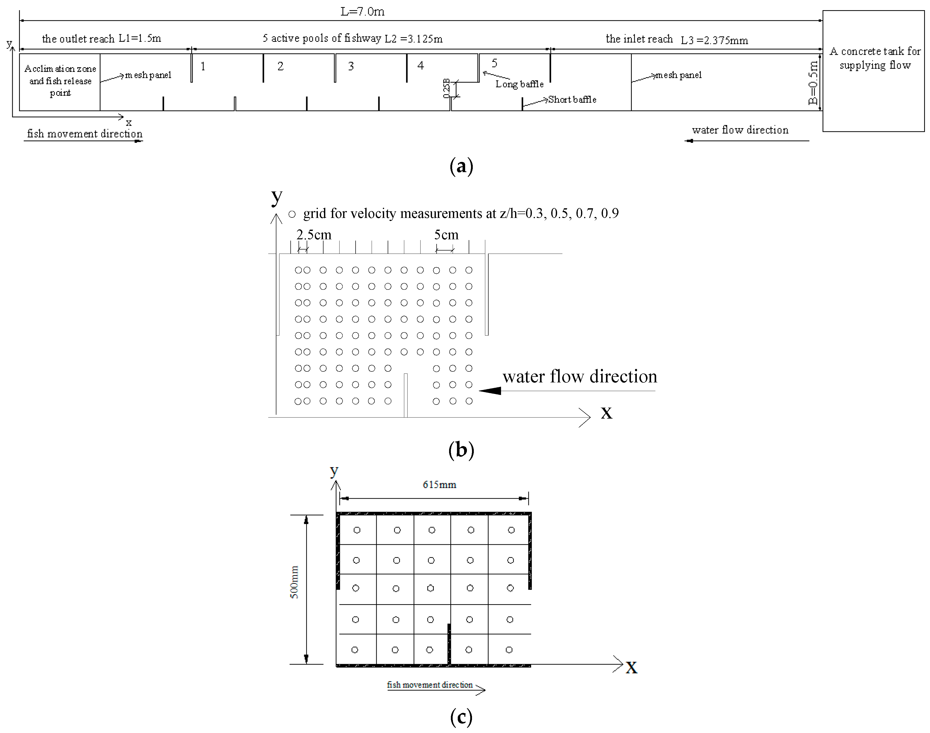
The geometry of the experimental fishway was 7 m (long) × 0.5 m (wide) × 0.7 m (high), externally strengthened by glass sidewalls, as shown in Figure 1a. The experimental fishway consisted of 5 active pools; the dimensions of each pool were 0.625 m (length) × 0.5 m (width) × 0.7 m (height). The fishway had long and short baffles positioned on one side of the sidewall. The inflow reach of the fishway was 2.375 m long, and a concrete tank that was 2.0 m (long) × 1.2 m (wide) × 1.5 m (high) located at the inflow reach of the fishway provided a smooth flow. An acclimation zone (0.7 m × 0.5 m × 0.7 m) was constructed 0.8 m downstream of the first pool. The water elevations in the vertical-slot fishway (VSF) were measured using a point gauge with ±0.1 mm accuracy. The slope of the fishway was 1%.
In the fishway, the domestic water supply was used in the experiments and recirculated through the laboratory pumping system (maximum capacity of 300 L/s). Temperature, pH, dissolved oxygen and dechlorination were recorded at the beginning and end of the experiments. VSF discharge was controlled by a water pump located at the upstream tank. The water surface levels were measured using a point gauge with ±0.1 mm accuracy. Three-dimensional instantaneous velocity components (x, y, z) in Pool 3 were measured with a SonTek 16 MHz Micro Acoustic Doppler Velocimeter (ADV, SonTek Inc., San Diego, USA) with a total of 102 points in each horizontal plane located 0.025–0.05 m apart to avoid touching the sidewalls with the probe, as shown in Figure 1b. The sampling frequency of the ADV was 50 Hz for a sampling period of 60 s for each point. The measurements were taken at different horizontal planes parallel to the flume bottom, namely, at 30%, 50%, 70% and 90% of the pool’s mean water depth, or z = 0.3 h, 0.5 h, 0.7 h and 0.9 h (where h is the pool mean water depth). Therefore, 408 points were measured in Pool 3. Filtering was used to remove samples with low correlation scores or signal-to-noise ratios. Instantaneous measures of velocity were filtered using the Goring and Nikora (2002) [30] phase-space threshold despiking as modified by Wahl (2002) [31].
All experimental silver carp (for a detailed description of silver carp, see Table 1) were supplied by Yidu hatchery (Yichang city, China). The fish were kept in a circular fish tank. To recover from the stress of transport, the fish were kept in the fish tank for at least 3 days before experiments started. To facilitate the positioning of the test fish, a reference grid containing 25 contiguous sequentially numbered cells (each 0.125 m × 0.1 m) were formed and used for fish behavior observation on the bottom of all of the pools (Figure 1c). When starting an experiment, the mesh panel in the outlet section was removed to obtain the fish’s voluntary movement. Each individual experiment lasted 1.5 h according to a preliminary experiment [29]. Experiments were conducted under the previously tested hydraulic conditions using one fish each time. The movement trajectories of fish were continuously recorded by a video recording system, which was mainly composed of one 25 fps digital video camera (DS-2CD3345-I, Hikvision Corporation, Hangzhou, China), video recorder (DS-7808N-K1/C, Hikvision Corporation) and computer. Logger Pro software (Vernier Software & Technology, Beaverton, OR, USA) was used to track the fish’s continuous positions, swimming velocity in the fishway and residence time spent by a fish at any location. After the test, the total body length and weight of each fish were measured.
2.2. Fish Response to Hydraulics
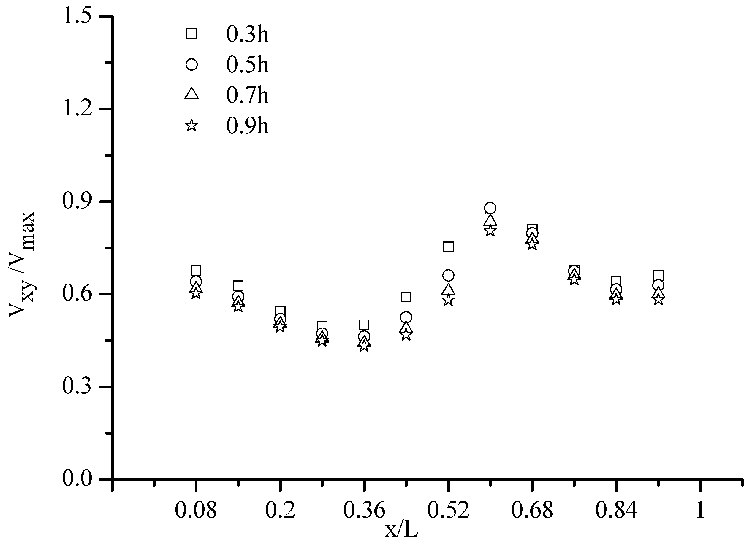
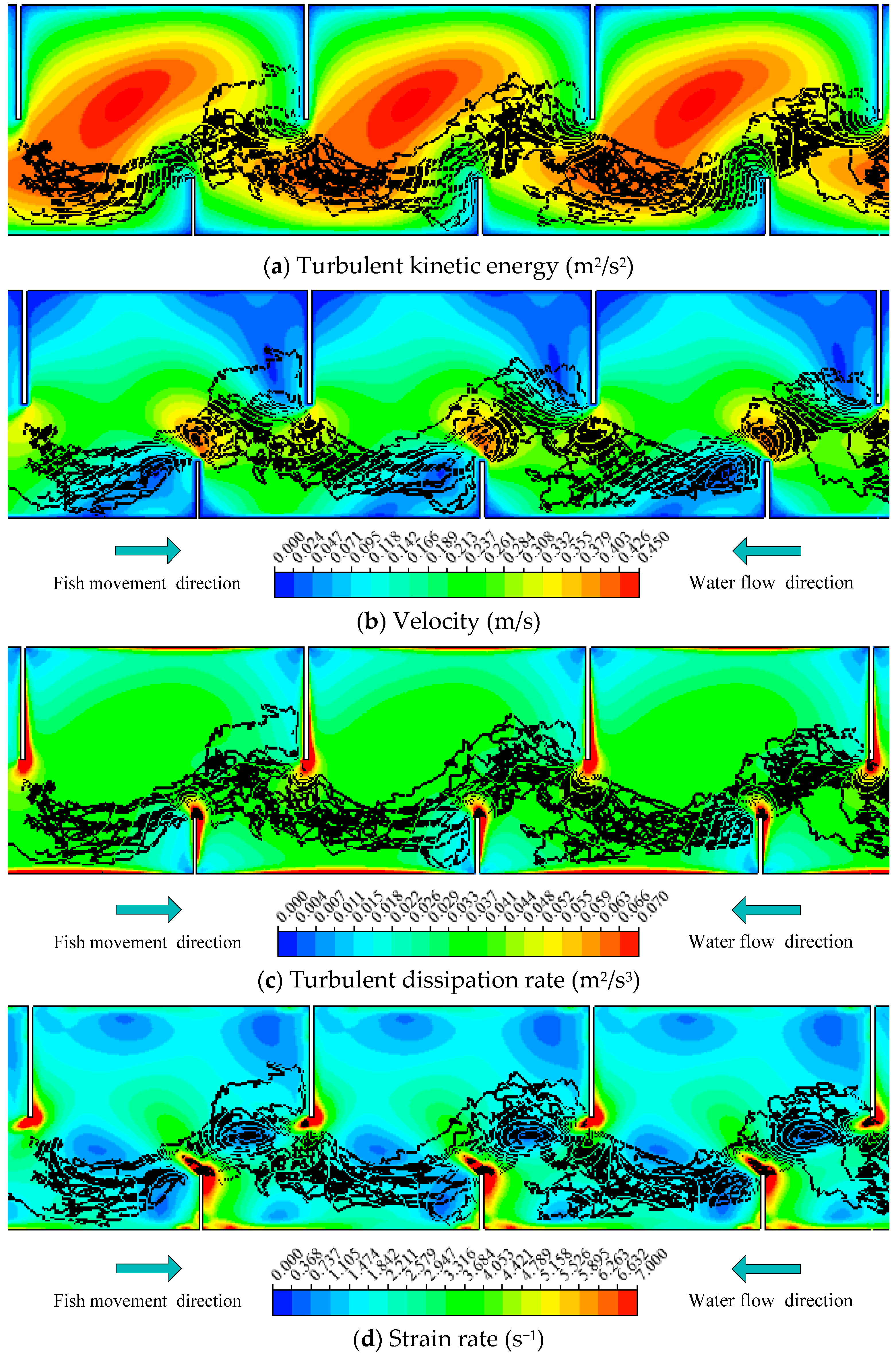
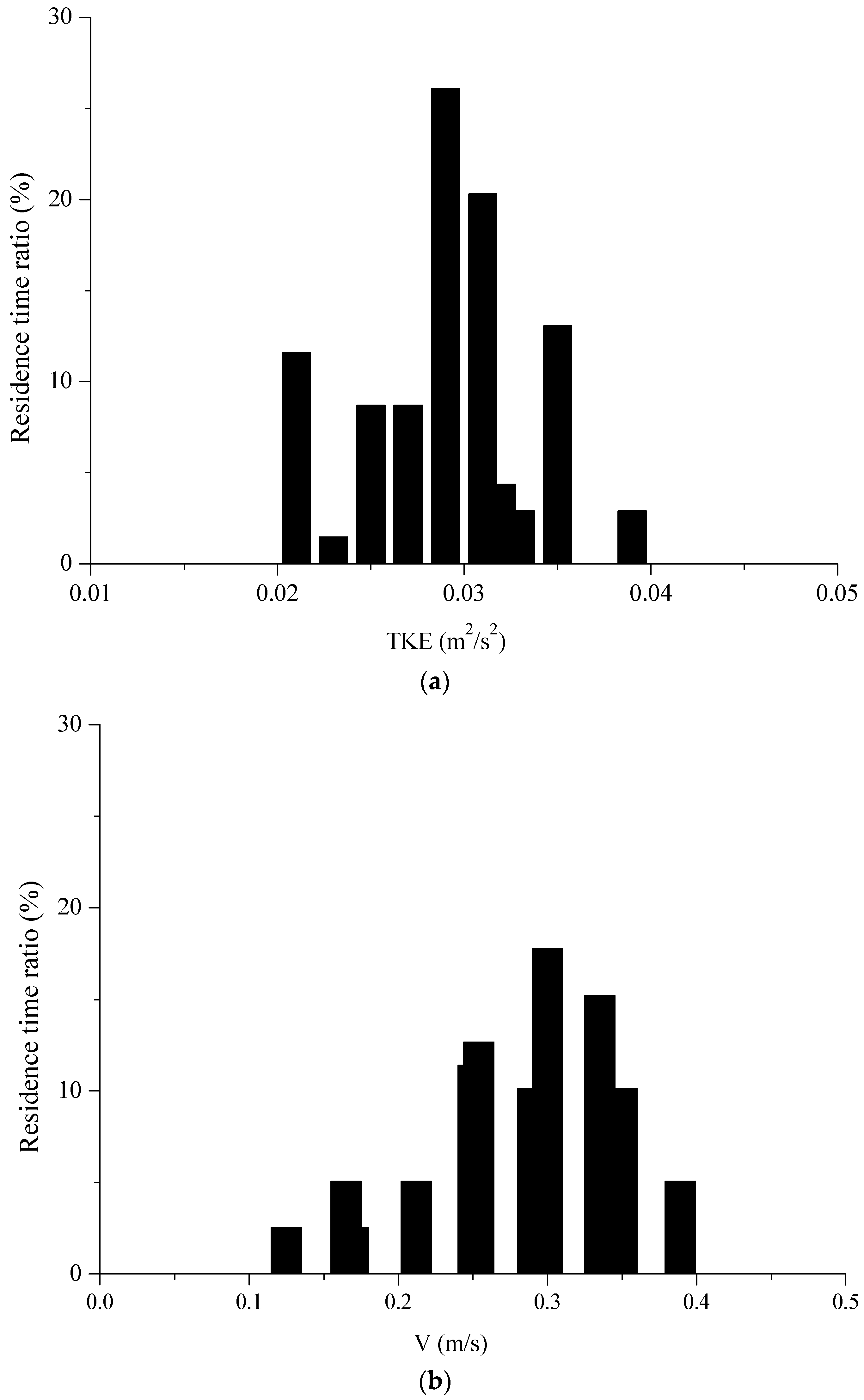
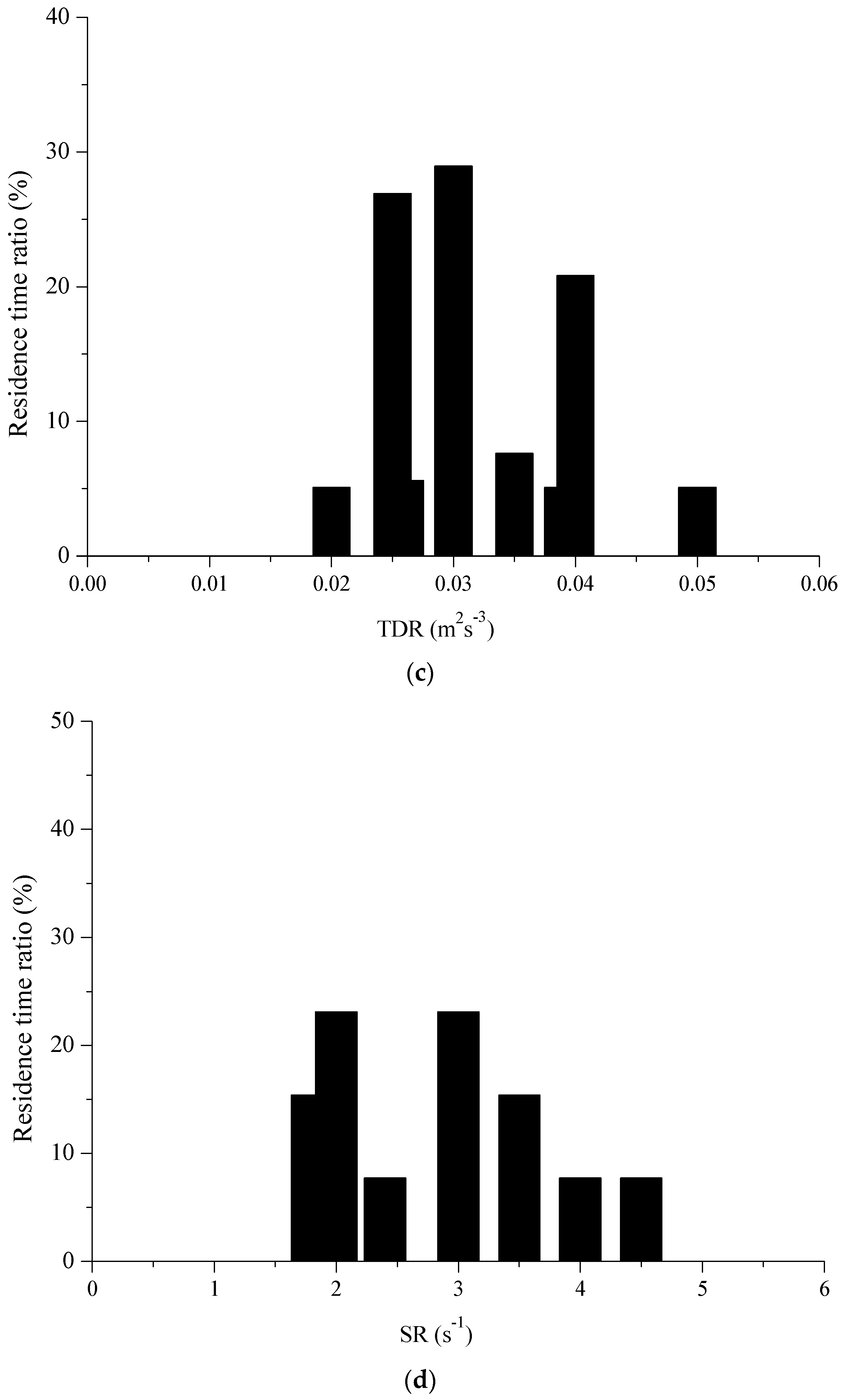
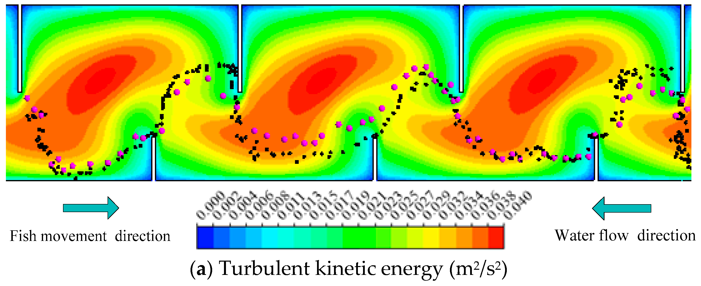
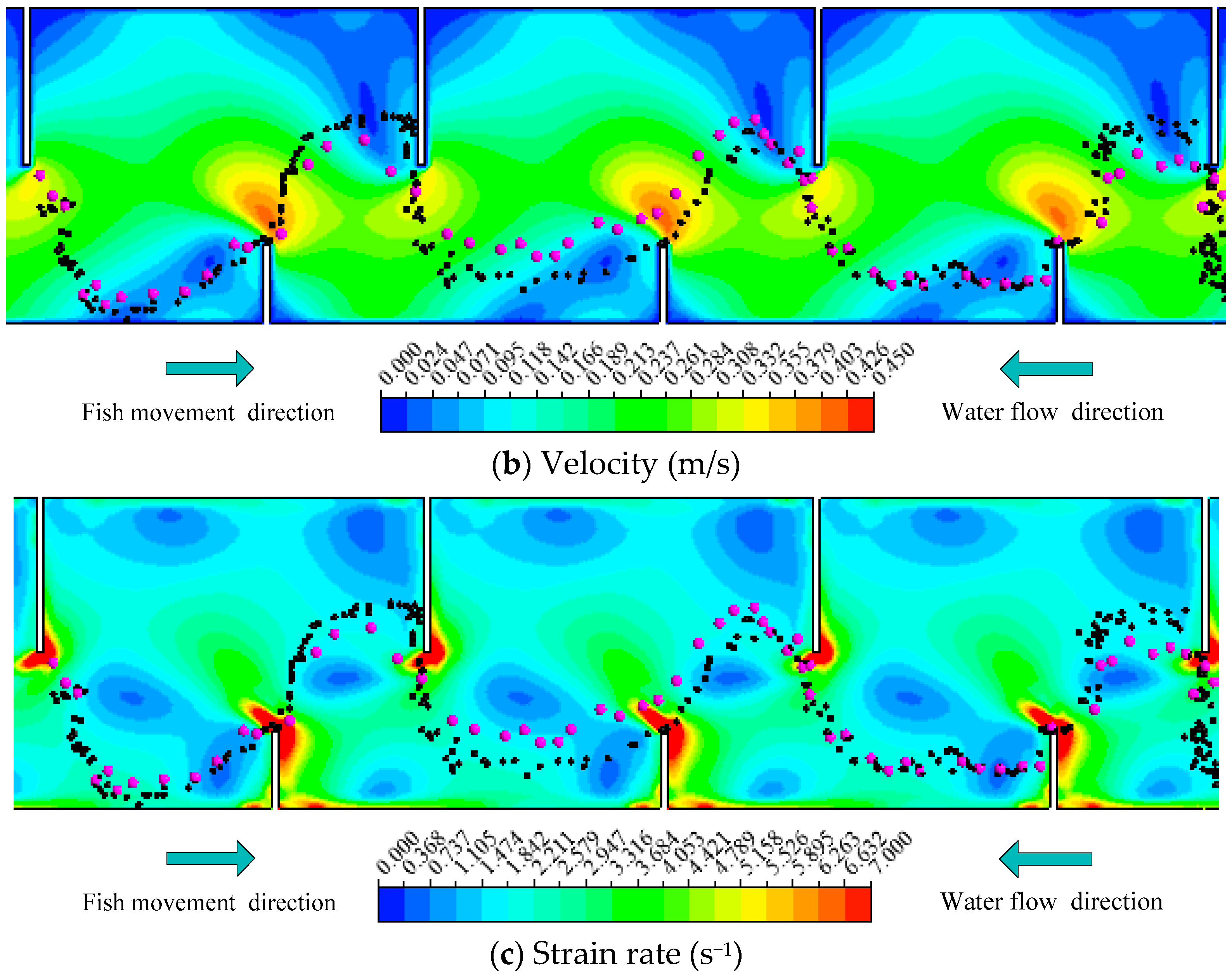
The dimensionless velocity in Pool 3 in four horizontal planes (z = 0.3 h, 0.5 h, 0.7 h and 0.9 h) is shown in Figure 2 with Q = 13.5 L/s, which have similarity in four horizontal planes. The fish movement trajectories, swimming velocity and residence times were tracked in the experimental fishway using the aforementioned method. The water depth was 0.3 m, and the recirculating discharge was set at 0.135 m3/s. In total, 30 individuals’ trajectories were obtained for fish that successfully passed from the first pool to the fifth one. The time (mean ± S.D.) for the fish to successfully pass through Pool 1 to Pool 5 was 19.61 ± 8.17 s for silver carp. The experimental fish trajectories in the VSF were combined with the hydraulic parameters shown in Figure 3. According to Figure 4, we concluded that the fish spent more time in the hydraulic stimulus range of TKE, V, TDR and SR, that were 0.02~0.035 m2/s2, 0.16~0.4 m/s, 0.023~0.042 m2/s3 and 1.8~4 s−1, respectively.
A good relationship between a hydraulic variable and the residence times indicated the hydraulic response of fish [23]. Therefore, Spearman’s correlation analysis was used to analyze the correlation between the residence time of individual fish and hydraulic parameters. From Figure 3a, the silver carps mainly used ranges of TKE between 0.02 and 0.035 m2/s2. The TKE and carps’ residence times were correlated (r = 0.507, p < 0.01). Among the other tested hydraulic parameters, a relationship between V and the residence time of carps was found (r = 0.440, p < 0.01). Accordingly, an association between the carps’ residence times and SR was found (r = −0.394, p < 0.01). By contrast, a very low relationship was found for TDR and the residence time of silver carp (r = −0.171, p < 0.01), although the fish remained in the areas with TED values from 0.023 to 0.042 m2/s3.
3. Fish Movement Trajectories Model
The fish movement was considered to be a two-step process: First, the fish evaluates all agents within the detection range of its sensory system, then, the fish responds to an agent by moving [32]. Although what a fish perceives is undoubtedly complex, it is believed that fish movement is mainly driven by a hydraulic stimulus [12,21]. The fish movement trajectories model was determined using a hydrodynamic model with an Eulerian framework and an individual-based fish movement-response model [33].
3.1. Hydrodynamic Model
The hydrodynamic model is composed of Reynolds-averaged Navier-Stokes (RANS) equations coupled with a standard RNG k-ε turbulence model. Recently, the hydraulic characteristics of fishways have been studied [4,12,26,34,35]. It is widely acknowledged that the flow field in a VSF can be approximated as a two-dimensional (2D) flow when the bed slope is small. Fish movements preferentially occurred close to the bottom of the VSF in the present study, suggesting that the fish trajectories varied largely in the horizontal plane. Therefore, we obtained the xy-plane hydraulic distribution of whole fishway from the hydrodynamic model. For brevity, the fish movement behavior was considered to be mainly affected by hydraulic parameters, which were provided as inputs to the fish model. On the basis of the experimental results presented in Section 2, the TKE, V and SR acted as hydraulic stimulus variables and the hydraulic stimulus ranges of these variables for the silver carp were applied to model fish movement in a fishway.
3.2. Fish Movement-Response Model
The individual-based fish movement-response model considers each individual fish, explores individual heterogeneity and tracks the movement position in a Lagrangian system [33]. In the model, the fish position was decided by the movement of the fish relative to the flow. The fish movement response depended on the hydraulic stimulus generated in the fishway without considering visual cues from, or tactile contact with, solid/wall structures.
3.2.1. Response Scopes
Commonly, a fish evaluates all hydraulic stimuli in the sensory area, which in a three-dimensional space can be partitioned into horizontal and vertical components, for the convenience of analysis and simulation, also named the sensory circle [12,21]. Here, we only need to consider the horizontal movement (2D sensory area) of the fish in a 2D flow field. The fish movement model mainly consisted of the response scope (sensory circle) and movement behavior. The radius of the sensory circle was defined as the sensory query distance (SQD) [21]. SQD represents the sensory range of the fishs’ lateral line mechanosensory system. SQD is a function of fish length, longer fish are able to detect hydraulic stimuli from greater distances [33]. However, the actual range depends on a number of factors including size and form of the disturbance source like hydraulic complexity and other factors [33]. We adopt the definition of SQD proposed by Goodwin et al. (2006) [21]:
where SQDb and SQDCFD are the biological and CFD-model sensory query distances, respectively. The biological sensory query distance is determined by means of the fish body length Lf, the operating range of the fish sensory system Da in a 1.0-s time increment, and the time increment . Goodwin et al. (2006) [21] stated that SQDCFD was larger than SQDb and SQD fluctuates randomly between 100% and 150% of SQDCFD by trial and error. It is generally thought that the “active space” (range) of the lateral line mechanosensory system (here a mechanical perception system of fish was only considered to simulate responses to flow in the model) is a function of fish length (1 to 2 body lengths Lf). It was reported that randomness was a fundamental feature of animal choices [36]. Gao et al. (2016) [12] indicated that the fish will make a response to an agent at a distance of about one fish body length with random fluctuations. We modified the SQD proposed by Gao et al. (2016) [12] according to the experimental data:
where Lf is the fish body length and RN is a random variable (0 < RN < 1) related to the fish body length Lf.
SQD = Lf·(1 + 0.75·RN)
3.2.2. Fish Movement Rules
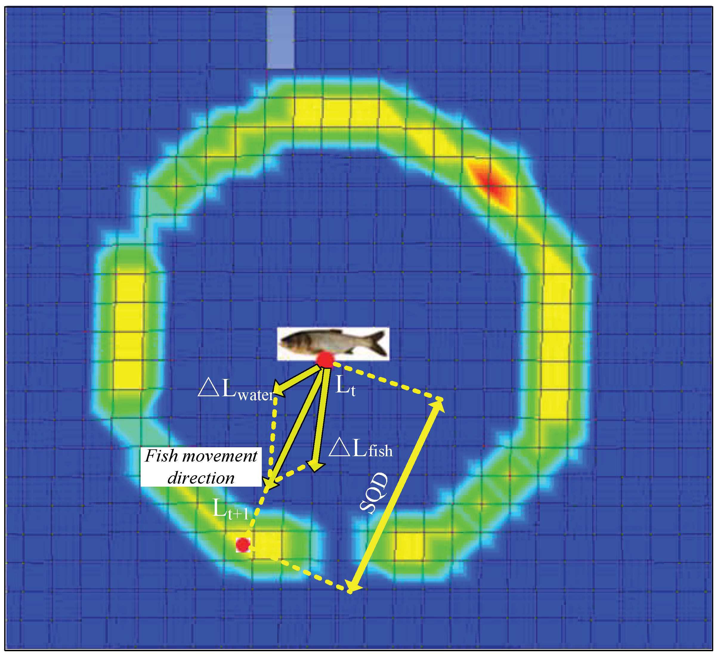
The movement rules determine how fish respond to external hydraulic changes and how they interacted with each other [37]. The refinement of the movement rules was based on experiments (Figure 3 and Figure 4). Taking the 3-dimensional hydrodynamic model as inputs and using the defined sensory circle, a Gaussian probability distribution was used to illustrate the response probability density functions [13]. A probability distribution, as seen in Equation (2), which is usually assumed to be Gaussian for mathematical convenience, can be used to illustrate behavior responses in the presence of different hydraulic stimuli. Figure 5 represents the sensory circle (response scopes) of the fish. The fish is located in the centre (red point) of this circle at a given moment. The individual always moves within the response scope, and the fish need to evaluate the hydraulic stimuli (here is comprehensive probability of hydraulic stimulus) at its location. The stimulus uses a cumulative model (Equation (5)). Fish will preferentially move into the mesh cells having the largest comprehensive probability within the response scope. When the largest comprehensive hydraulic stimuli are found simultaneously both upstream and downstream, the fish will always select the upstream mesh cell(s) considering the fish’s positive rheotaxis. Unless the fish cannot find any upstream stimuli, it will select a downstream one. In Figure 5, if fish found the hydraulic stimuli with largest comprehensive probability at the lower left (using a red point), the path from the center to the red point of lower left determines the direction of the fish movement. The distance between the two red points is SQD. Furthermore, when an individual fish was close to the boundary, a solid wall, the individual had to redirect its movement direction to avoid striking the wall.
where f(xi) (i = 1, 2, 3) is the probability of each hydraulic variable, xi is the actual hydraulic value, μs is the preference hydraulic value, F is comprehensive probability of hydraulic stimulus, Wi is the influence coefficient of each hydraulic factor, and the sum of W is 1.
In the present computational model, the model was constrained that the fish movement distance cannot exceed the SQD in each time step Δt. Bian [32] stated that when the fish determined the detection in its sensory system, then the fish responds to an agent by moving. That means the fish always move into the largest comprehensive hydraulic stimulus which is perceived within the sensory circle.
The movement distance L of an individual fish within the period of one time increment Δt can be expressed by the displacement vector, which is the resultant of the flow and fish swimming:
The displacement of water was defined as the water velocity vector and the time increment Δt. The water velocity vector at the fish position was interpolated from the hydrodynamic model grid. was the average swimming velocity of fish, was the water velocity where the fish have been in the response circle. It means that the fish swim with similar velocity in each of pool. Therefore, the resultant velocity was not representative of the actual efforts made by the fish and only relevant to the actual swimming velocity. In the future, we hope to establish a relationship between the physiological indices like bio-energetic costs of fish and the kinetic parameters like Lfish, Vfish in the fishway.
According to our experiment, the average ascending time of individual fish in each sensory circle was assumed to be approximately 0.3 s. The model parameters used are summarized in Table 2. To validate the movement rules of fish, the fish movement trajectories model was applied to the experimental fishway.
4. Results
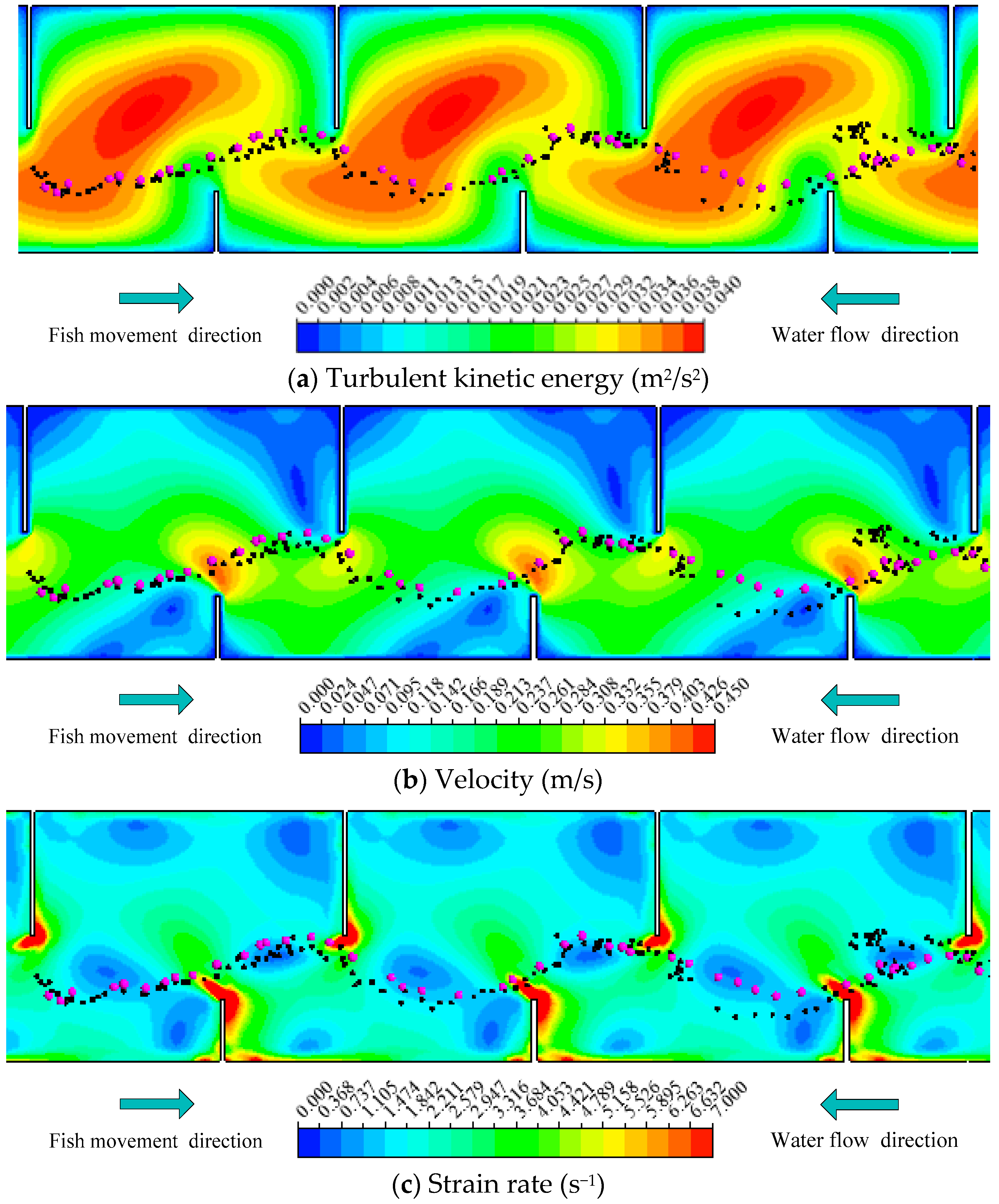
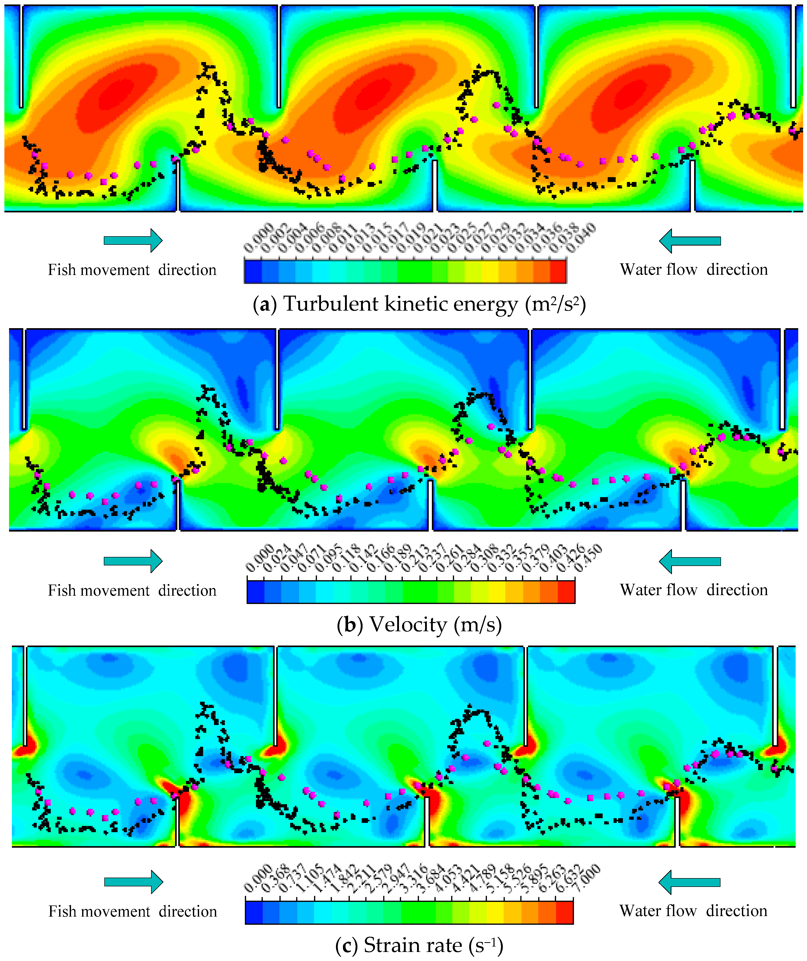
To assess the fish movement rules, the model was validated and calibrated with data from the experimental fishway (Figure 1). The choice of model parameters is summarized in Table 2 and will now be justified. The three representative measured fish trajectories, namely, Fish A (a carp 12.1 cm long), Fish B (a carp 11.7 cm long) and Fish C (a carp 12.2 cm long) are separately displayed using black points in Figure 6, Figure 7 and Figure 8. The rose red points represent the simulated fish movement trajectories. The simulated trajectories start at the fish release point. We just presented the trajectories in Pools 2–4, which are clearly showed in the video camera and have similar flow conditions. Fish A avoided the high TKE areas in the pools and moved along the lower part of the pools (Figure 6). Fish B chose a longer path (Figure 7) and persistently passed the pools through all the baffles. Fish C adopted the upper and lower staggered paths to ascend the pools (Figure 8), just like Fish B, but with a longer path. Moreover, although the mean flow field and turbulence level were nearly the same in Pools 2–4, the real measured fish trajectories presented different routes through the pools. These results suggest that the choice of fish through a pool was random (just like the random variable RN in Equation (3)). The comparison of all observed fish movement trajectories in the experimental VSF and simulated ones, which showed similar patterns with relatively little difference for all trajectories, lent plausibility to the fish movement rules.
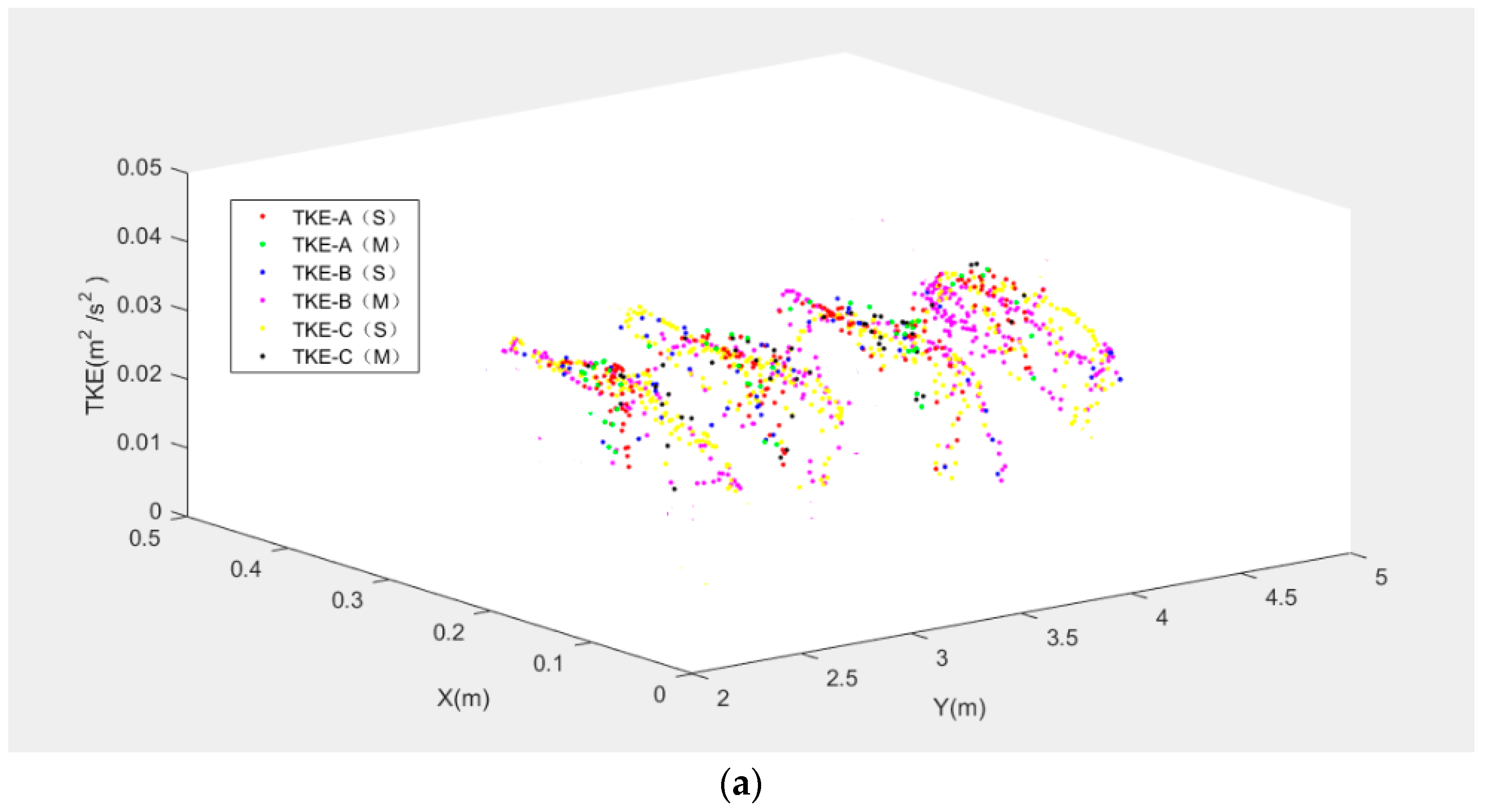
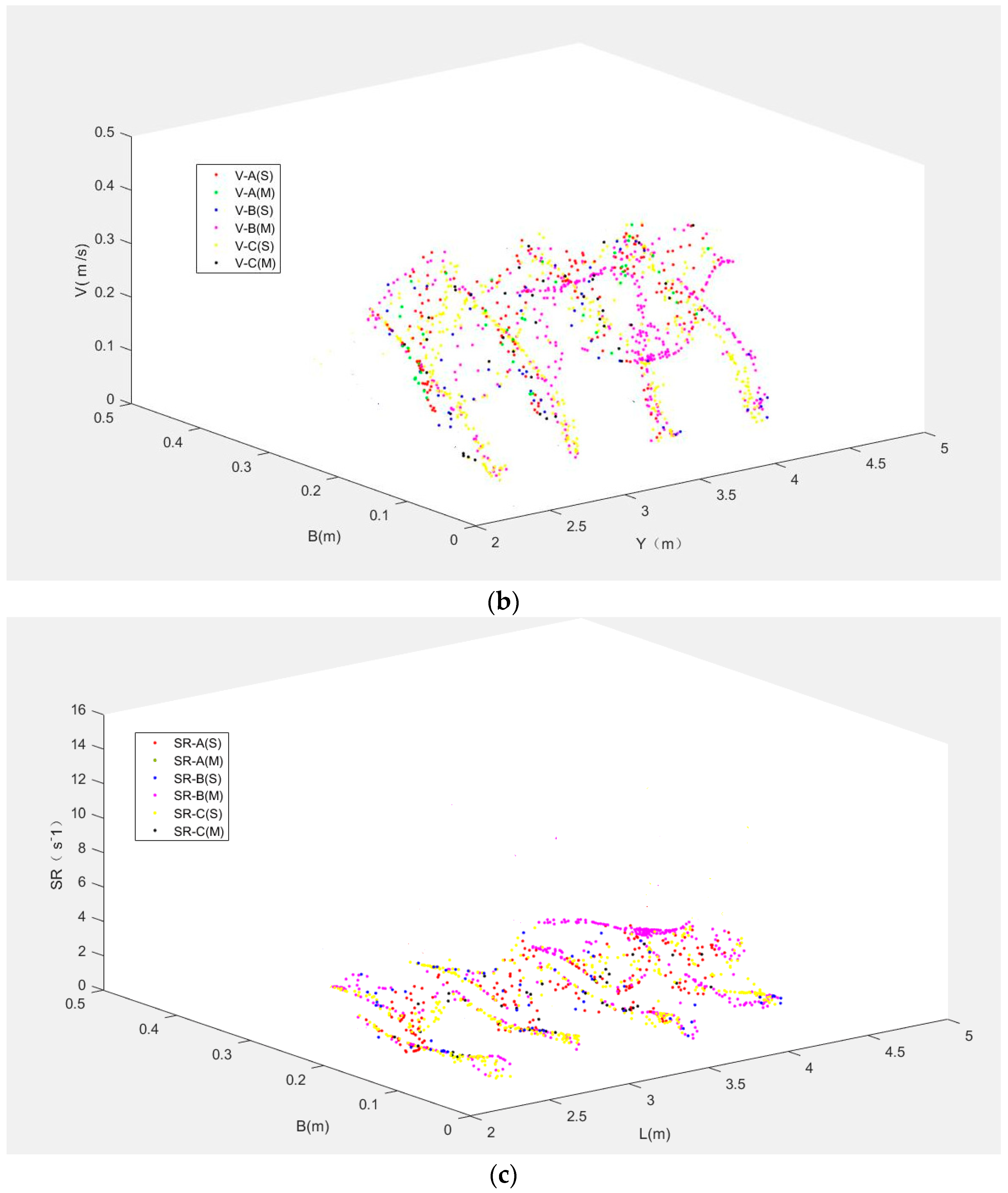
In addition, the results of V, TKE, SR for Fish A, B and C using different graphs were shown to see the difference in Figure 9. Figure 9a was the differences in TKE for Fish A, B and C between the simulated and measured trajectories. The tendency of TKE was largely similar for the simulated and measured trajectories for the three fish. In Figure 9b,c, the simulated and measured trajectories for Fish A, B and C had similar trend lines. It was further confirmed that the movement rules and response scope can be used to track fish trajectories in this model.
5. Discussion
The primary goal of this study was to predict the silver carps’ trajectories considering the hydraulic stimulus variables TKE, V and SR in a 1% vertical slot fishway at a discharge of 13.5 L/s using a modified version of an IBM. The IBM fish movement trajectories model is a coupling method to integrate, understand and simulate fish movement considering hydraulic conditions in order to present a single fish movement process in the response scope. The model has the advantage of using defined rules for fish movement and behavior. The model can efficiently characterize the individual properties and actions of the fish. The property differences were represented by the length, and the action difference was represented by the movement and response to the hydraulic conditions [21]. Yet, the model was tested in a VSF with very specific and repeating hydraulic conditions. If so, more different hydraulic conditions and enough variability in length should be considered to test and quantify the model’s accuracy.
The main purpose of a fishway is to provide a flow path through which a fish is willing and physically capable of swimming through. Yet, the fish of various species and sizes which can find, enter, and safely swim through a fishway quickly enough, and do not disrupt their life cycles, was important. In this paper, the flow condition did not exceed the fish’s swimming ability (critical or burst speed), and the fish could use the flow condition to find a path through which they are capable of swimming. It is suggested that the hydraulic stimulus variables are important to determine carps’ movements in a fishway. TKE, V and SR were considered as hydraulic stimuli (abiotic factors) in the present model. TKE had the greatest effects, with an influence coefficient (WTKE) of 0.412 on fish’s upstream trajectories in this type of fishway (Table 2). V and SR had influence coefficients (WV and WSR) of 0.391 and 0.197, respectively. The present study regarded that fish only respond to the proposed hydraulic stimulus metrics, but it could be possible that fish could be responding to meso-scale hydraulic features such as velocity gradients, circulation, vorticity, etc., [38,39] in flow. Further studies may be performed to quantify the exact types of energy gradients, vortex or circulation structures that different fish species are utilizing. Better understanding of the interaction between fish behavior and the characteristics of different hydraulic metrics will provide insights into judging fishway design.
In this model, the available data from the experimental fishway preliminary demonstrated the plausibility of the model results, but did not allow a deeper calibration due to the lack of a large number of measured movement trajectories. The accuracy and the application scopes for this model still need to be improved. It is urgent to carry out experimental and, especially, field studies using different lengths of wild fish to get fish movement trajectories, fish swimming velocities, movement behaviors, etc. The present experiment did not consider fish themselves different swimming abilities, other hydraulic and environmental variables, such as water quality, dissolved oxygen, substrate, temperature, etc., [40], and disregard that some fish unsuccessfully pass through the fishway not in the range of video camera monitoring, and that the simulated fish movement trajectories were slightly different from the experimental ones. These variables should be further studied to improve the experimental results.
Biotic indicator-physiological indices [41] can show fish movement behavior such as energy costs and mortality. It was possible to survey physiological boundary conditions using an experimental method such as PIT-tagged or radio-tagged techniques [42], electromyogram telemetry (EMG) [43,44] to get the physiological indices in our model. Just like the hydrodynamic boundary conditions used in CFD, the physiological boundary conditions at the entrance to the numerical fishway were considered [12]. The variation of physiological indices was tracked along the particular trajectory followed by an individual fish in the whole swimming period in order to explore the differential movement behavior. It is useful to evaluate the fishway passage efficiency and the post-passage. Prospectively, further models may be able to integrate the mentioned abiotic and biotic factors (physiological indices) to improve the accuracy of the simulation.
Evaluating fishway passage efficiency was the end objective for modeling of fish trajectories. Accuracy is also an important feature of any evaluation method for fishway passage efficiency. Although there are some limitations in this model, it appears that this methodology has potential merit. Traditional methods for evaluating fishway passage were based only on single or simple hydraulic indices such as the maximum velocity or energy dissipation in a pool, the velocity distribution, turbulence characteristics of the flow, which did not consider the interaction between fish behavior and multiple hydraulic variables. Our modeling approach is essentially from real experimental approaches to accurately model parameters. Once enough reliable model parameters become available, we believe that our model can be used to estimate the fish passage efficiency nearly as accurately as an experiment and definitely better than traditional evaluation methods.
6. Conclusions
In this paper, a modified IBM movement trajectories model was developed coupling hydraulic stimulus variables TKE, V and SR and fish movement behavior rules to model the silver carps’ trajectories in a 1% vertical slot fishway at a discharge of 13.5 L/s. Although some of the parameters involved in the present modeling are uncertain or even completely unknown, the simulated and measured trajectories preliminary implied the plausibility of the model movement rules. The end objective of the fish trajectories modeling was predicting and evaluating fishway passage efficiency, and accuracy is an important element. So, it is essential to carry out long-term monitoring in the field.
Author Contributions
All authors listed have contributed substantially to the manuscript to be included as authors. J.T., L.T., Z.G. and X.S. had a substantial involvement in the conception, guidance, and revising of the manuscript. J.T., Z.G. and H.D. were involved in the design and data acquisition in the laboratory work. The data analysis and interpretation was done in collaboration with all authors, as was the final approval of the version to be published. J.T., L.T., G.Z. wrote the manuscript. All authors read and approved the final version of the manuscript.
Funding
This study has been supported by the National Natural Science Foundation of China (51709152, 51579136), and Open Research Fund of State Key Laboratory of Simulation and Regulation of Water Cycle in River Basin (China Institute of Water Resources and Hydropower Research) (IWHR-SKL-201616).
Acknowledgments
The anonymous reviewers provided more suggestions for the model and encouraged us to better describe the discussion, thanks for their suggestions and comments.
Conflicts of Interest
The authors declare no conflict of interest.
References
- Schilt, C.R. Developing fish passage and protection at hydropower dams. Appl. Anim. Behav. Sci. 2007, 104, 295–325. [Google Scholar] [CrossRef]
- Shi, X.; Kynard, B.; Liu, D.; Qiao, Y.; Chen, Q. Development of fish passage in China. Fisheries 2015, 40, 161–169. [Google Scholar] [CrossRef]
- Kim, J.H.; Yoon, J.D.; Baek, S.H.; Park, S.H.; Lee, J.W.; Lee, J.A.; Jang, M.H. An efficiency analysis of a nature-like fishway for freshwater fish ascending a large Korean river. Water 2015, 8, 3. [Google Scholar] [CrossRef]
- Puertas, J.; Cea, L.; Bermúdez, M.; Pena, L.; Rodriguze, A.; Rabunal, J.R.; Balairon, L.; Lara, A.; Aramburu, E. Computer application for the analysis and design of vertical slot fishways in accordance with the requirements of the target species. Ecol. Eng. 2012, 48, 51–60. [Google Scholar] [CrossRef]
- Marriner, B.A.; Baki, A.B.M.; Zhu, D.Z.; Thiem, J.D.; Cooke, S.J.; Katopodis, C. Field and numerical assessment of turning pool hydraulics in a vertical slot fishway. Ecol. Eng. 2014, 63, 88–101. [Google Scholar] [CrossRef]
- An, R.; Li, J.; Liang, R.; Tuo, Y. Three-dimensional simulation and experimental study for optimising a vertical slot fishway. J. Hydro-Environ. Res. 2016, 12, 119–129. [Google Scholar] [CrossRef]
- Blake, R.W. Fish functional design and swimming performance. J. Fish Biol. 2004, 65, 1193–1222. [Google Scholar] [CrossRef]
- Newbold, L.R.; Shi, X.; Hou, Y.; Han, D.; Kemp, P.S. Swimming performance and behaviour of bighead carp (Hypophthalmichthysnobilis): Application to fish passage and exclusion criteria. Ecol. Eng. 2016, 95, 690–698. [Google Scholar] [CrossRef]
- Castro-Santos, T.; Shi, X.; Haro, A. Migratorybehavior of adult sea lamprey and cumulative passage performance through four fishways. Can. J. Fish. Aquat. Sci. 2017, 74, 790–800. [Google Scholar] [CrossRef]
- Romão, F.A.; Santos, J.M.; Katopodis, C.; Pinheiro, A.N.; Branco, P. How does season affect passage performance and fatigue of potamodromous Cyprinids? An Experimental Approach in a vertical slot fishway. Water 2018, 10, 395. [Google Scholar] [CrossRef]
- Rodriguez, A.; Bermudez, M.; Rabunal, J.R.; Puertas, J.; Dorado, J.; Pena, L.; Balairon, L. Optical fish trajectory measurement in fishways through computer vision and artificial neural networks. J. Comput. Civ. Eng. 2011, 25, 291–301. [Google Scholar] [CrossRef]
- Gao, Z.; Andersson, H.I.; Dai, H.; Jiang, F.; Zhao, L. A new Eulerian-Lagrangian agent method to model fish paths in a vertical slot fishway. Ecol. Eng. 2016, 88, 217–225. [Google Scholar] [CrossRef]
- Kemp, P.S.; Anderson, J.J.; Vowles, A.S. Quantifying behaviour of migratory fish: Application of signal detection theory to fisheries engineering. Ecol. Eng. 2012, 41, 22–31. [Google Scholar] [CrossRef]
- Haefner, J.W.; Bowen, M.D. Physical-based model of fish movement in fish extraction facilities. Ecol. Model. 2002, 152, 227–245. [Google Scholar] [CrossRef]
- Arenas, A.; Politano, M.; Weber, L.; Timko, M. Analysis of movements and behavior of smolts swimming in hydropower reservoirs. Ecol. Model. 2015, 312, 292–307. [Google Scholar] [CrossRef]
- Glas, M.; Tritthart, M.; Zens, B.; Keckeis, H.; Lechner, A.; Kaminskas, T.; Habersack, H. Modelling the dispersal of riverine fish larvae: From a raster-based analysis of movement patterns within a racetrack flume to a rheoreaction-based correlated random walk (RCRW) model approach. Can. J. Fish. Aquat. Sci. 2017, 74, 1474–1489. [Google Scholar] [CrossRef]
- DeAngelis, D.L.; Gross, L.J. Individual-Based Models and Approaches in Ecology; Chapman and Hall: New York, NY, USA, 1992. [Google Scholar]
- Han, R.; Chen, Q.; Blanckaert, K.; Li, W.; Li, R. Fish (Spinibarbus hollandi) dynamics in relation to changing hydrological conditions: Physical modelling, individual-based numerical modelling, and case study. Ecohydrology 2013, 6, 586–597. [Google Scholar] [CrossRef]
- Li, W.; Han, R.; Chen, Q.; Qu, S.; Cheng, Z. Individual-based modeling of fish population dynamics in the river downstream under flow regulation. Ecol. Inform. 2010, 5, 115–123. [Google Scholar] [CrossRef]
- Yu, W.; Chen, X.; Li, Y. Review on individual-based model in fishery science. Mar. Fish. 2012, 34, 464–475. (In Chinese) [Google Scholar] [CrossRef]
- Goodwin, R.A.; Nestler, J.M.; Anderson, J.J.; Weber, L.J.; Loucks, D.P. Predicting 3-D fish movement behavior using a Eulerian-Lagrangian-agent method (ELAM). Ecol. Model. 2006, 192, 197–223. [Google Scholar] [CrossRef]
- Haro, A.; Castro-Santos, T.; Noreika, J.; Odeh, M. Swimming performance of upstream migrant fishes in open-channel flow: A new approach to predicting passage through velocity barriers. Can. J. Fish. Aquat. Sci. 2004, 61, 1590–1601. [Google Scholar] [CrossRef]
- Silva, A.T.; Santos, J.M.; Ferreira, M.T.; Pinheiro, A.N.; Katopodis, C. Effects of water velocity and turbulence on the behaviour of Iberian barbel (Luciobarbusbocagei, Steindachner 1864) in an experimental pool-type fishway. River Res. Appl. 2011, 27, 360–373. [Google Scholar] [CrossRef]
- Yagci, O. Hydraulic aspects of pool-weir fishways as ecologically friendly water structure. Ecol. Eng. 2010, 36, 36–46. [Google Scholar] [CrossRef]
- Enders, E.C.; Boisclair, D.; Roy, A.G. A model of total swimming costs in turbulent flow for juvenile Atlantic salmon. Can. J. Fish. Aquat. Sci. 2005, 62, 1079–1089. [Google Scholar] [CrossRef]
- Tarrade, L.; Texier, A.; David, L.; Larinier, M. Topologies and measurements of turbulent flow in vertical slot fishways. Hydrobiologia 2008, 609, 177–188. [Google Scholar] [CrossRef] [Green Version]
- Liao, J.C. A review of fish swimming mechanics and behavior in altered flows. Philos. T. Roy. Soc. Lon. 2007, 362, 1973–1993. [Google Scholar] [CrossRef] [PubMed]
- Silva, A.T.; Katopodis, C.; Santos, J.M.; Ferreira, M.T.; Pinheiro, A.N. Cyprinid swimming behaviour in response to turbulent flow. Ecol. Eng. 2012, 44, 314–328. [Google Scholar] [CrossRef]
- Tan, J.; Gao, Z.; Dai, H.; Shi, X. The correlation analysis between hydraulic characteristics of vertical slot fishway and fish movement characteristics. J. Hydraul. Eng. 2017, 48, 924–932. (In Chinese) [Google Scholar] [CrossRef]
- Goring, D.G.; Nikora, V.I. Despiking acoustic Doppler velocimeter data. J. Hydraul. Eng. 2002, 128, 117–126. [Google Scholar] [CrossRef]
- Wahl, T.L. Discussion of ‘‘Despiking acoustic Doppler velocimeter data”. J. Hydraul. Eng. 2002, 129, 484–487. [Google Scholar] [CrossRef]
- Bian, L. The representation of the environment in the context of individual-based modeling. Ecol. Model. 2003, 159, 279–296. [Google Scholar] [CrossRef]
- Coombs, S. Signal detection theory, lateral-line excitation patterns and prey capture behaviour of mottled sculpin. Anim. Behav. 1999, 58, 421–430. [Google Scholar] [CrossRef] [PubMed]
- Rajaratnam, N.; Katopodis, C.; Solanki, S. New design for vertical slot fishways. Can. J. Civ. Eng. 1992, 19, 402–414. [Google Scholar] [CrossRef]
- Wu, S.; Rajaratnam, N.; Katopodis, C. Structure of flow in vertical slot fishway. J. Hydraul. Eng. 1999, 125, 351–360. [Google Scholar] [CrossRef]
- Farnsworth, K.D.; Beecham, J.A. How do grazers achieve their distribution? Acontinuum of models from random diffusion to the ideal free distribution usingbiased random walks. Am. Nat. 1999, 153, 509–526. [Google Scholar] [CrossRef] [PubMed]
- Ristroph, L.; Liao, J.C.; Zhang, J. Lateral line layout correlates with the differential hydrodynamic pressure on swimming fish. Phys. Rev. Lett. 2015, 114, 018102. [Google Scholar] [CrossRef] [PubMed]
- Crowder, D.W.; Diplas, P. Applying spatial hydraulic principles to quantify stream habitat. River Res. Appl. 2006, 22, 79–89. [Google Scholar] [CrossRef]
- Shen, Y.; Diplas, P. Application of two-and three-dimensional computational fluid dynamics models to complex ecological stream flows. J. Hydrol. 2008, 348, 195–214. [Google Scholar] [CrossRef]
- Bravo-Córdoba, F.J.; Sanz-Ronda, F.J.; Ruiz-Legazpi, J.; Celestino, L.F.; Makrakis, S. Fishway with two entrance branches: Understanding its performance for potamodromous Mediterranean barbels. Fish. Manag. Ecol. 2018, 25, 12–21. [Google Scholar] [CrossRef]
- Pon, L.B.; Hinch, S.G.; Cooke, S.J.; Patterson, D.A.; Farrell, A.P. Physiological, energetic and behavioural correlates of successful fishway passage of adult sock-eye salmon Oncorhynchus nerka in the Seton River, British Columbia. J. Fish Biol. 2009, 74, 1323–1336. [Google Scholar] [CrossRef] [PubMed]
- Calles, O.; Greenberg, L. Connectivity is a two-way street—The need for aholistic approach to fish passage problems in regulated rivers. River Res. Appl. 2009, 25, 1268–1286. [Google Scholar] [CrossRef]
- Hinch, S.G.; Standen, E.M.; Healey, M.C.; Farrell, A.P. Swimming patterns and behavior of upriver-migration adult pink (Oncorhynchus gorbuscha) and sockeye (O. nerka) salmon as assessed by EMG telemetry in the Fraser River, British Columbia, Canada. Hydrobiologia 2002, 483, 147–160. [Google Scholar] [CrossRef]
- Pon, L.B.; Hinch, S.G.; Cooke, S.J.; Patterson, D.A.; Farrell, A.P. A comparison of the physiological condition, and fishway passage time and success ofmigrant adult sockeye salmon at Seton River Dam, British Columbia, under threeoperational water discharge rates. N. Am. J. Fish. Manag. 2009, 29, 1195–1205. [Google Scholar] [CrossRef]
Figure 1.
(a) The planform of the first experimental vertical-slot fishway (VSF); (b) the measured points in each horizontal plane in one pool of the first experimental VSF; (c) reference grid that was used for observing the fish behavior in one pool.
Figure 1.
(a) The planform of the first experimental vertical-slot fishway (VSF); (b) the measured points in each horizontal plane in one pool of the first experimental VSF; (c) reference grid that was used for observing the fish behavior in one pool.

Figure 2.
Dimensionless velocity distribution curves in y = 0.225 m along the x direction in four different horizontal planes with Q = 13.5 L/s (Vmax represents maximum V in the slot, Vxy represents the velocity in xy-plane, x is the distance along x-direction in one pool, L is the length of a pool).

Figure 3.
The representative movement trajectories of silver carp in Pools 2–4 combined with hydraulic parameters with Q = 13.5 L/s (Z = 0.3 h): (a) Turbulent kinetic energy (TKE); (b) Velocity (V); (c) Turbulent dissipation rate (TDR); (d) Strain rate (SR) in the experimental fishway.
Figure 3.
The representative movement trajectories of silver carp in Pools 2–4 combined with hydraulic parameters with Q = 13.5 L/s (Z = 0.3 h): (a) Turbulent kinetic energy (TKE); (b) Velocity (V); (c) Turbulent dissipation rate (TDR); (d) Strain rate (SR) in the experimental fishway.

Figure 4.
Hydraulic curves for silver carp based on observed residence times in the experimental VSF: (a) TKE; (b) V; (c) TDR; (d) SR.
Figure 4.
Hydraulic curves for silver carp based on observed residence times in the experimental VSF: (a) TKE; (b) V; (c) TDR; (d) SR.


Figure 5.
Illustration of fish movement rules of the model.

Figure 6.
Representative trajectory of Fish A combined with (a) TKE; (b) V; (c) SR distribution in Pools 2–4 (Notes: The rose red points represent the simulated fish movement trajectories, and the black points represent the measured trajectories of fish).
Figure 6.
Representative trajectory of Fish A combined with (a) TKE; (b) V; (c) SR distribution in Pools 2–4 (Notes: The rose red points represent the simulated fish movement trajectories, and the black points represent the measured trajectories of fish).

Figure 7.
Representative trajectory of Fish B combined with (a) TKE; (b) V; (c) SR distribution in Pools 2–4 (Notes: The rose red points represent the simulated fish movement trajectories, and the black points represent the measured trajectories of fish).
Figure 7.
Representative trajectory of Fish B combined with (a) TKE; (b) V; (c) SR distribution in Pools 2–4 (Notes: The rose red points represent the simulated fish movement trajectories, and the black points represent the measured trajectories of fish).

Figure 8.
Representative trajectory of Fish C combined with (a) TKE; (b) V; (c) SR distribution in Pools 2–4 (Notes: The rose red points represent the simulated fish movement trajectories, and the black points represent the measured trajectories of fish).
Figure 8.
Representative trajectory of Fish C combined with (a) TKE; (b) V; (c) SR distribution in Pools 2–4 (Notes: The rose red points represent the simulated fish movement trajectories, and the black points represent the measured trajectories of fish).


Figure 9.
The differences between simulated (S) and measured (M) trajectories for Fish A, B and C: (a) TKE; (b) V; (c) SR.
Figure 9.
The differences between simulated (S) and measured (M) trajectories for Fish A, B and C: (a) TKE; (b) V; (c) SR.


Table 1.
Detailed description of experimental conditions.
| Location | Q (L/s) | h (m) | N | Total Length (cm) | Total Weight (g) |
|---|---|---|---|---|---|
| Fishway | 13.5 | 0.3 | 30 (silver carp) | 11.49 ± 0.63 | 20.74 ± 8.64 |
Notes: Total length and total weight is the mean ± S.D. value.
Table 2.
The model parameters.
| Parameter | Model Validation and Calibration |
|---|---|
| Individuals | Model validation (27 individuals) and calibration (3 individuals) |
| Average moving time in each sensory circle | 0.3 s |
| The hydraulic stimulus range of TKE | 0.02–0.035 m2/s2 |
| The hydraulic stimulus range of V | 0.2–0.4 m/s |
| The hydraulic stimulus range of SR | 1.5–3.5 s−1 |
| WTKE | 0.412 |
| WV | 0.391 |
| WSR | 0.197 |
| Response scopes | Lf·(1 + 0.75·RN) |
Notes: Lf is the fish body length.
© 2018 by the authors. Licensee MDPI, Basel, Switzerland. This article is an open access article distributed under the terms and conditions of the Creative Commons Attribution (CC BY) license (http://creativecommons.org/licenses/by/4.0/).
Share and Cite
MDPI and ACS Style
Tan, J.; Tao, L.; Gao, Z.; Dai, H.; Shi, X. Modeling Fish Movement Trajectories in Relation to Hydraulic Response Relationships in an Experimental Fishway. Water 2018, 10, 1511. https://doi.org/10.3390/w10111511
AMA Style
Tan J, Tao L, Gao Z, Dai H, Shi X. Modeling Fish Movement Trajectories in Relation to Hydraulic Response Relationships in an Experimental Fishway. Water. 2018; 10(11):1511. https://doi.org/10.3390/w10111511
Chicago/Turabian StyleTan, Junjun, Lin Tao, Zhu Gao, Huichao Dai, and Xiaotao Shi. 2018. "Modeling Fish Movement Trajectories in Relation to Hydraulic Response Relationships in an Experimental Fishway" Water 10, no. 11: 1511. https://doi.org/10.3390/w10111511
Note that from the first issue of 2016, this journal uses article numbers instead of page numbers. See further details here.