Assessment of Precipitation Simulations in Central Asia by CMIP5 Climate Models


1
State Key Laboratory of Desert and Oasis Ecology, Xinjiang Institute of Ecology and Geography, Chinese Academy of Sciences, Urumqi 830011, China
2
College of Resource and Environment Sciences, Xinjiang University, Urumqi 830046, China
3
Xinjiang Institute of Ecology and Geography, University of Chinese Academy of Sciences, Beijing 100049, China
*
Author to whom correspondence should be addressed.
Water 2018, 10(11), 1516; https://doi.org/10.3390/w10111516
Submission received: 16 July 2018
/
Revised: 20 October 2018
/
Accepted: 20 October 2018
/
Published: 25 October 2018
(This article belongs to the Special Issue The Future of Water Management in Central Asia)
Abstract
:The Coupled Model Intercomparison Project Phase 5 (CMIP5) provides data, which is widely used to assess global and regional climate change. In this study, we evaluated the ability of 37 global climate models (GCMs) of CMIP5 to simulate historical precipitation in Central Asia (CA). The relative root mean square error (RRMSE), spatial correlation coefficient, and Kling-Gupta efficiency (KGE) were used as criteria for evaluation. The precipitation simulation results of GCMs were compared with the Climatic Research Unit (CRU) precipitation in 1986–2005. Most models show a variety of precipitation simulation capabilities both spatially and temporally, whereas the top six models were identified as having good performance in CA, including HadCM3, MIROC5, MPI-ESM-LR, MPI-ESM-P, CMCC-CM, and CMCC-CMS. As the GCMs have large uncertainties in the prediction of future precipitation, it is difficult to find the best model to predict future precipitation in CA. Multi-Model Ensemble (MME) results can give a good simulation of precipitation, and are superior to individual models.
1. Introduction
Climate change presents a range of challenges for agriculture, forest, and water management practices [1]. A large number of studies have shown that climate change can also significantly affect the distribution of water resources. Therefore, governments should also make corresponding adjustments in the planning and management policies of water resources [2,3]. Climate change has a significant impact on the distribution of water resources in space and time, which will make a great difference in precipitation in different seasons and regions, and also affect the amount of water resources. As a key climate variable, precipitation plays a crucial role in the water cycle [4]. Therefore, current and future water-related issues are major national and international relations issues, which means that it is especially important to evaluate the magnitude and change in precipitation [5].
In the past several decades, there have been a variety of studies using global climate models to explore climate change in different areas and aspects. Most models overestimate precipitation in Africa and Asia, but in Europe, these show low biases. However, the ability of the climate models to simulate precipitation in Central Asia (CA) is still unknown. Assessing and quantifying future precipitation changes is one of the fundamentals for developing future water management and planning strategies in CA; thus, it is critical to use some metrics to perform the evaluation of climate models. As reported by Gleckler et al. [6], the assessment of the performance of climate models should not only focus on the average state; it is necessary to evaluate the performance of climate models more comprehensively. Later, some new climate model metrics were proposed by Moise [7].
Chen and Frauenfeld [8], using three future emission scenarios: Representative Concentration Pathway (RCP) 8.5, RCP 4.5, RCP 2.6 to estimate the spatial pattern of precipitation over China during the 20th century, found that Coupled Model Intercomparison Project Phase 5 (CMIP5) is better than CMIP3 at simulating the spatial and temporal distribution of precipitation in China [8]. For the continental areas between the latitudes 60 degrees north and 60 degrees south, the models captured the characteristics of the temperature better than precipitation during 1930–2004 [9]. Twenty-five CMIP5 global climate models (GCMs) were chosen to evaluate and compare the simulation of climate models for precipitation and temperature over central Africa and found that most CMIP5 models are better at simulating temperature than precipitation [10]. Huang et al. assessed the CMIP5 summer precipitation and found that the multi-model ensemble can reproduce summer precipitation over eastern China [11]. As shown by the study in East Asia, the characteristics of summer rainfall have been reproduced by CMIP5 [12]. Comparing the CMIP3 and CMIP5 simulation of the Asian monsoon, CMIP5 reasonably captures the characteristics of the Asian monsoon in winter [13]. So far, global climate models are the most reliable way to predict future climate change, and there are also differences between models [14,15].
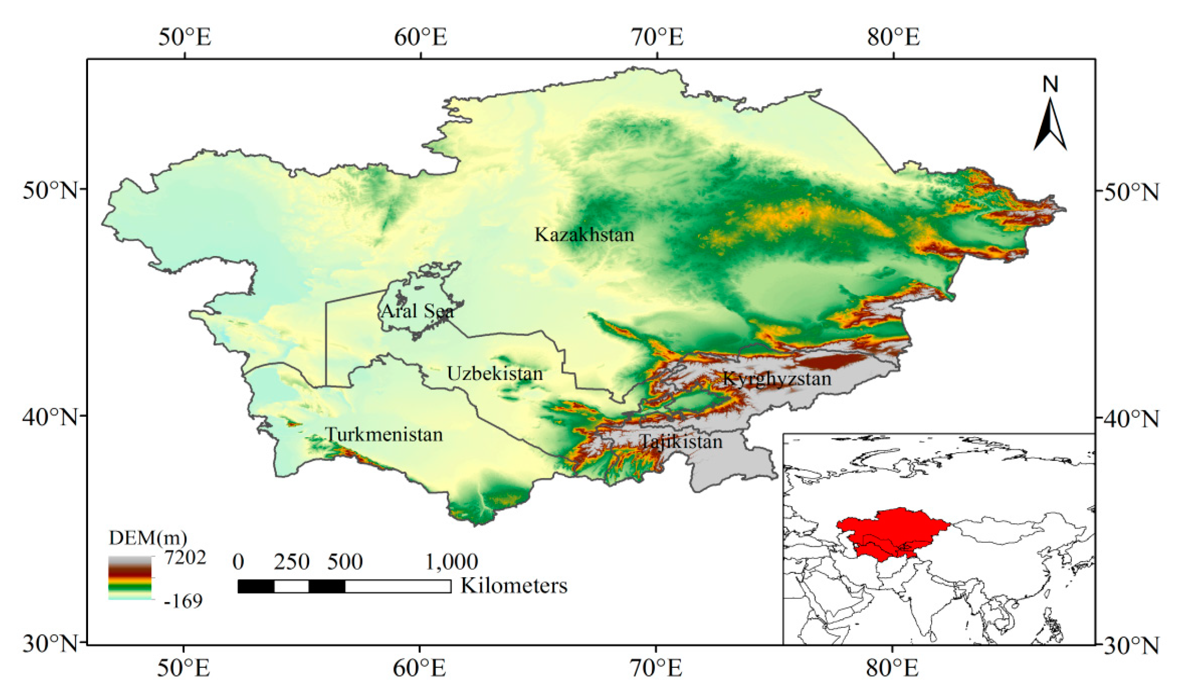
CA (Figure 1) is usually specified as five central Asian countries, namely Kazakhstan, Turkmenistan, Uzbekistan, Tajikistan, and Kyrgyzstan. CA covers an area of about 4 million square kilometers, and the population is about 60 million [16]. CA has arid and semi-arid regions. Its climate is a typical temperate continental climate, where the precipitation is scarce, sunlight sufficient, the temperature changes violently, and the ecology and environment are fragile and sensitive to climate change [17]. Its water resources are irreplaceable strategic resources, which restrict the production of industry and agriculture and affect the relationship between the five countries. With continued global warming, there is a lack of systematic research on the future trends of climate change and their spatial and temporal distribution of characteristics in CA. Therefore, studying the climate characteristics of CA in the future is of great significance for understanding climate change in CA and making the corresponding decisions in response to climate change.
The spatial correlation coefficient was generally used to compare the major Empirical Orthogonal Functions (EOFs), which are derived from GCMs data and observation [18,19,20,21]. Kioutsioukis et al. applied the root mean square error (RMSE) to compare the differences between models and observation [22]. The Kling–Gupta efficiency (KGE) has been demonstrated to be superior the Nash–Sutcliffe efficiency [23]. In this study, we investigated precipitation simulations over the CA regions with relative root mean square error (RRMSE) and the spatial correlation coefficient, based on the 37 GCMs from CMIP5 models in the historical experiment (years 1986–2005). Our research focuses on the following questions: (1) Can GCMs reproduce the characteristics of precipitation in Central Asia? (2) Which models can better simulate precipitation in CA and can be used to predict future precipitation variation in CA? Additionally, the assessment of precipitation simulations from CMIP5 models in CA can provide better corresponding measures for future water resource management and planning strategies.
2. Data
Thirty-seven global climate models were selected in this study. Table 1 lists information about climate models, including the name of the modeling center, its institute ID, and its horizontal resolution. The monthly mean precipitation data in the historical experiment was selected for research. The duration of historical experiment data is from 1850 to 2005, but we followed the Intergovernmental Panel on Climate Change (IPCC) 5th Assessment Report and selected the reference period from 1986 to 2005 (from http://cmip-pcmdi.llnl.gov/cmip5/index.html).
This work also uses Climatic Research Unit (CRU) time-series (TS) v4.01 precipitation data as observation data. This dataset has a spatial resolution of 0.5° × 0.5°. The CRU dataset was updated earlier by Mitchell and Jones, and their purpose was to construct a database of monthly climate observations from meteorological stations [24]. The CRU dataset was widely used to assess model skill in simulation [25,26,27,28]. The CRU datasets have a high reliability, especially after 1930 in CA [29]. The dataset is available from http://www.cru.uea.ac.uk.
3. Methods
For ease of comparison, the CMIP5 model data and CRU TS v4.01 were remapped to a 0.5° × 0.5° grid by using bilinear interpolation [30]. The correlation coefficient was used between the observation and the simulation [31,32,33]. In order to compare the simulation capability of the precipitation interannual variability, the standard deviation was calculated between the simulation and observation. The root mean square error (RMSE) was calculated to quantify the accuracy of the CMIP5 model simulation [34,35,36,37]. The mean differences between the simulated and observed climate variable, can be described by RMSE. RMSE can be calculated as follows:
where and denote the observed and simulated precipitation, and is the number of pairs in the analysis.
The relative root mean square error (RRMSE) was calculated to measure a model’s performance relative to the other models, with respect to the observation.
where RMSEmedian is the median of RMSE for all individual models. The index RRMSE may vary from −1 to positive infinity. The smaller the RRMSE, the better the simulation effect. A negative RRMSE indicates that the corresponding model performs better than the majority (50%) of models [38].
If the correlation coefficient between the simulation and observation is higher than 0.75, we consider that the model simulates well [39].
The projected precipitation changes, both monthly and seasonal are summarized using box-and-whisker plots. These plots consist of the multi-model median, the interquartile model spread (the range between the 25th and 75th quantiles, box), and the full inter-model range (whiskers). The multi-model median is taken to be the projected change, while the interquartile model spread and inter-model range visualize uncertainties in the projection and can also indicate model agreement or disagreement on the direction of the projected change.
For higher-level comparison, empirical orthogonal function (EOF) analysis is applied to investigate the spatial variations of precipitation. Over the past few decades, many studies have applied EOF analysis to derive the principle components of climate variability [40,41,42,43]. EOF analysis is a technique that is used to identify optimal representation of patterns (main signals). EOF analyses the precipitation data and reduces it to spatial patterns by its own EOFs, which explains most of the variance in precipitation. Moreover, EOF analysis produces a new set of orthogonal functions; this helps us to simplify the relevant factors efficiently [44]. In this study, the first two EOFs of thirty-seven models were retained and these share 90% of the total variance of the each model. The EOF analysis can be expressed simply as
where i = 1, …, m; j = 1, …, n; m is the number of grids; n is the time series length; xij are ith components of the jth random vector for the normalized data; Vki are the components of the eigenvectors of the correlation matrix; Zkj are the principal components. The first several leading EOFs can best represent the variance of precipitation. The EOFs can be understood as spatial standing waves. In the process of evolution, the precipitation at each grid increases or decreases but the spatial position remains the same. Besides, EOFs are arranged in descending order of variance, and they can capture the main information and exclude redundant information of the original data. The variance contribution rate is used to describe the percentage variance captured by each of EOFs. We use the following formula to calculate the variance contribution rate:
where p is the variance contribution rate, λ is the eigenvalue of covariance matrix, i is the number of eigenvalues, i = 1, …, n.
Statistical analysis of the comparison of models and observations is necessary. RRMSE, correlation coefficient, and Nash-Sutcliffe model efficiency were widely used to evaluate the goodness of fit between simulations and observations. However, their suitability as metrics has been questioned. The KGE considered the correlation coefficient, bias, and variability between simulations and observations, and the method proved to be more efficient than the commonly used Nash-Sutcliffe efficiency, while clearly time-sensitive. In addition, KGE solves the problems caused by the interactions between these components, such as the fact that variability is underestimated. In a perfect model with no data errors, the KGE value is equal to 1. Therefore, for better comparison between the CRU and CMIP5 models, we applied the Kling‒Gupta efficiency (KGE) approach to our research. The KGE was proposed by Gupta et al. [45]. The KGE can be described by
where r is the linear correlation in the simulated and observed values, α is the ratio of standard deviation of observed and simulated value, and β is the ratio of mean values of simulations and observations, s represents the simulations and o represents the observations.
The most widely used metrics for model evaluation are correlation coefficients, the mean squared error (MSE), root mean squared error (RMSE), and Nash-Sutcliffe efficiency (NSE). We added KGE into the metrics, which is a supplement to the correlation coefficient and RRMSE as the metrics. It is expected that the best climate model for precipitation simulation can be selected. In addition, KGE has been demonstrated to be more appropriate than NSE as metrics for model evaluation. Therefore, we consider that correlation coefficient, RMSE, and KGE are sufficient as metrics to select the optimal model.
In this study, the CRU data were collected for the period of 1986 to 2005, for comparison with the GCMs data. The monthly precipitation data were also accumulated to create the annual data. Besides, as we know, different models have different horizontal resolutions, which is troublesome. This makes it important to unify the horizontal resolution among different models. Kim et al. show that the details in the Climate model simulations of the monsoon demarcation were improved as the resolution increases [46]. The high-resolution simulations do obtain realistic distributions of precipitation; the position and amount of precipitation simulated by the higher resolution climate models are more consistent with observations than low-resolution simulations. The CMIP5 dataset is useful and widely relied on for assessing the future precipitation. However, CMIP5 projections conducted at a low horizontal resolution are difficult to use for determining crucial topographic effects and small-scale processes. This is why we chose the higher horizontal resolution grid. Thus, in order to facilitate the comparison with CRU, the monthly CMIP5 models precipitation were remapped to a resolution of 0.5°, identical with that of CRU.
4. Results
4.1. The Comparison of Observation and Simulation Using Conventional Statistics
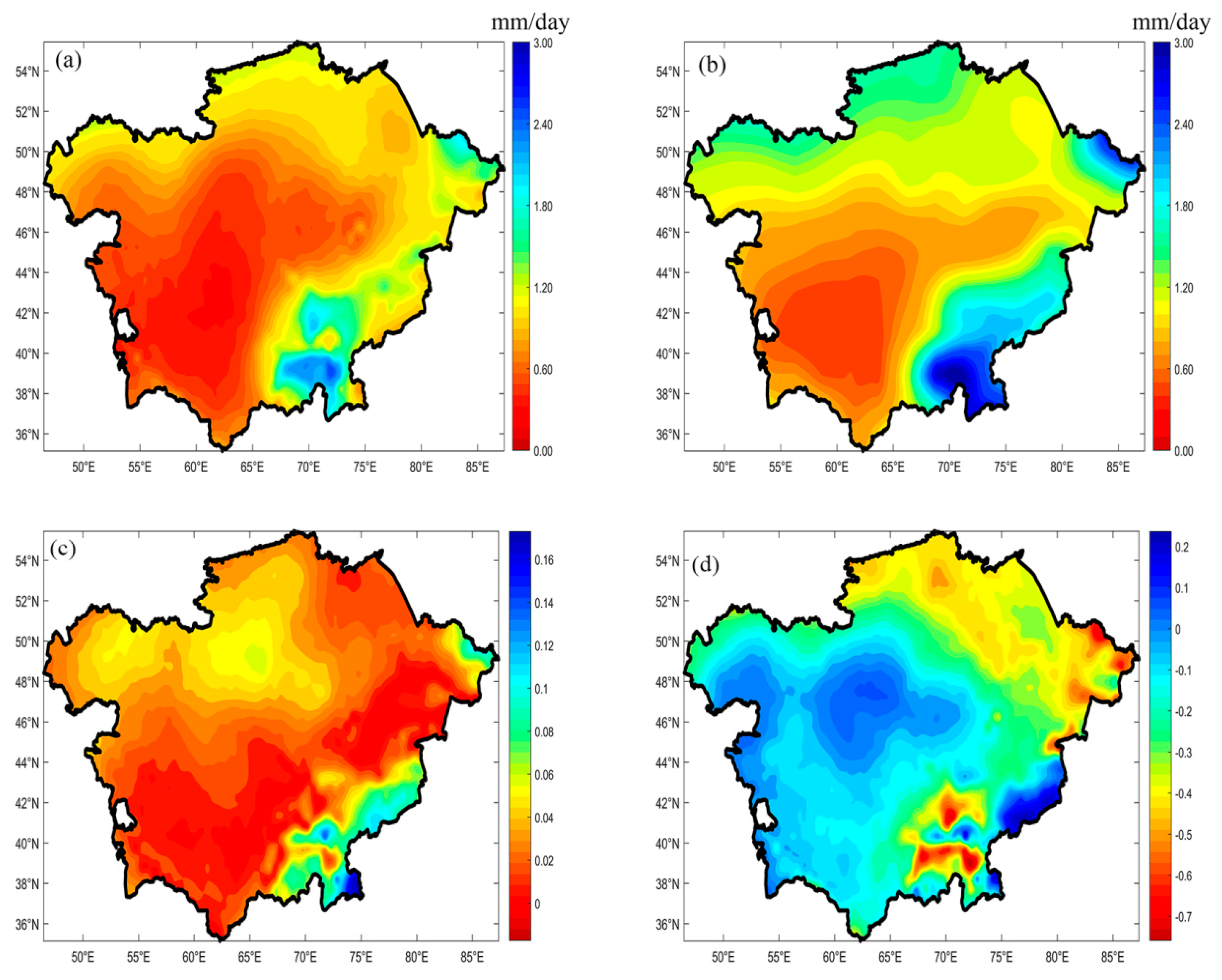
We first tested whether the CMIP5 models can reproduce the spatial distribution characteristics of precipitation based on the Multi-Model Ensemble (MME). Thus, we compared the spatial pattern of the observations and simulations from 1986 to 2005. Figure 2a shows the spatial distribution of mean annual precipitation in 1986–2005 from CRU and the MME (Figure 2b) from CMIP5. There is good agreement between the observation and simulation. The highest precipitation occurs over southeastern CA. The lowest precipitation is observed over southwestern CA, especially in Turkmenistan and Uzbekistan. In general, CMIP5 MME can reproduce the spatial distribution of annual precipitation reasonably in CA. However, compared with CRU, CMIP5 MME slightly overestimates the precipitation magnitude in many regions of CA (Figure 2a,b).
Figure 2c shows the RMSE of annual mean precipitation in 1986–2005 from the CMIP5 MME and CRU. As can be seen from Figure 2c, the RMSE of Uzbekistan and Turkmenistan is less than 0.02 mm/day, which shows that the CMIP5 MME can simulate the annual average precipitation in this area well. The RMSE of the eastern part of Kazakhstan is also below 0.02 mm/day. The RMSE of the northwestern part of Kazakhstan is about 0.06 mm/day, indicating that the climate model has slightly overestimated precipitation in this region. In Tajikistan and eastern Kyrgyzstan, the RMSE is about 0.1 mm/day. Especially in the Pamir area, the RMSE reaches the maximum of 0.17 mm/day, indicating that the CMIP5 MME also overestimated precipitation in this region. However, the RMSE in most of CA is below 0.04, indicating that CMIP5 MME can better simulate the historical precipitation characteristics of CA in 1986–2005. In order to assess the simulation capacity of CMIP5 MME on the interannual variability of precipitation, we calculated the difference of the standard deviation between CMIP5 MME and observation (MME minus CRU). As shown in Figure 2d, the high value center of precipitation interannual variability appears in eastern Kyrgyzstan and eastern Tajikistan. In contrast to Figure 2c, the interannual precipitation variation of the high value center and the RMSE of the high value area are basically consistent. In areas with a large precipitation, the interannual variability of precipitation is large.
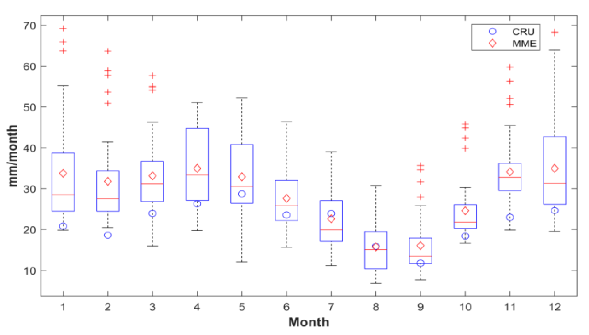
Figure 3 shows the box-and-whisker plot of the monthly average precipitation in CA from 1986 to 2005. The red diamond represents the mean values of MME, and the blue circle represents the mean values of observation. The blue box represents the maximum, upper quartile, median, lower quartile, and minimum of the precipitation simulated by MME.
It can be seen from Figure 3 that the MME can simulate the monthly variation characteristics of precipitation well. The simulated values of MME show the same variation characteristics as the observation. However, the monthly precipitation of the CA region simulated by the MME is slightly higher than the observation. Especially in February, MME overestimated the average precipitation and the difference between the MME and observation is 13.2 mm/month. The best simulation months of MME run from May to September, and the difference between the simulated value and the observed value is below 4.21 mm/month. Among them, the best simulation month is August, wherein the simulated value and the observed value are basically equivalent, the difference being 0.1 mm/month.
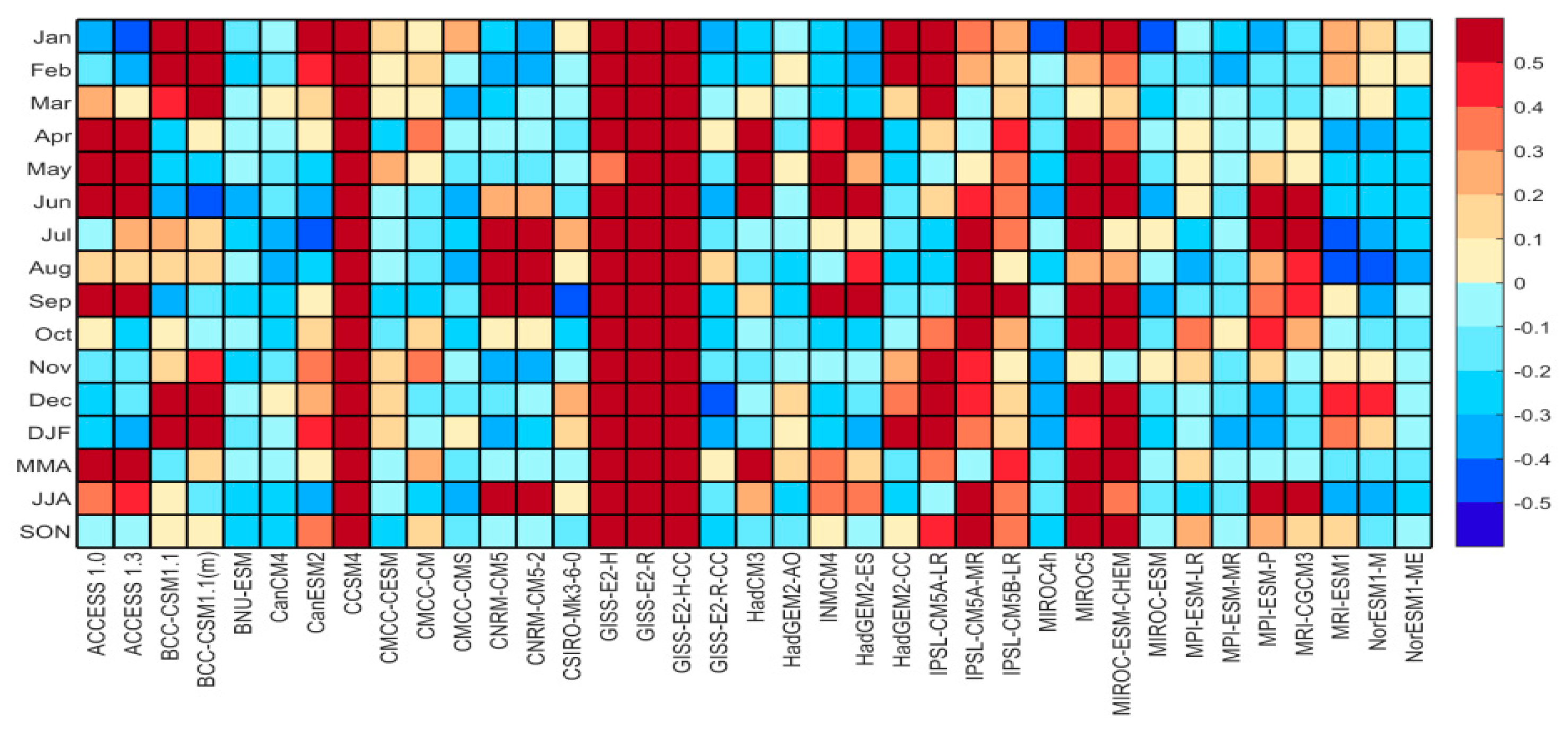
In order to assess the ability of each CMIP5 model in reproducing the observed climatological monthly and seasonal precipitation variations, we calculated the area-averaged monthly and seasonal RRMSE of precipitation from 1986 to 2005. It can be clearly seen from Figure 4 that the RRMSE is less than 0 (blue), which means that the simulation effect of this model is better than the median level of all models, and the RRMSE is greater than 0 (red), indicating that the simulation effect of this model is lower than the median. The simulation effect of precipitation at each time scale of CCSM4, GISS-E2-H, GISS-E2-H-CC, and GISS-E2-R is not good, indicating that the four CMIP5 models lack a basic simulation capability of precipitation over CA. The models with good simulation ability are BNU-ESM, CanCM4, CMCC-CESM, CMCC-CM, CMCC-CMS, and CSIRO-Mk3-6-0 and so on.
4.2. The Simulation of Historical Precipitation from 1986 to 2005 in Central Asia
Based on the monthly precipitation data of CRU from 1986 to 2005, EOFs were calculated, which represent the modes of interannual precipitation variability, and the eigenvectors and eigenvalues of the annual precipitation series were obtained. The variance contribute rate of the first two EOFs of CRU is 87.88%. In order to investigate whether two EOFs are independent of each other, this study used the North et al. equation 24 to evaluate if eigenvalues are significantly separated [47]. Among them, the variance contribution rate of EOF1 is 74.09% and EOF2 is 13.79%, both passing the significance test. The main characteristic of EOF1 is that all the Central Asian regions show positive signals (Figure 5a). The high-value center is located in Tajikistan and the low-value center is located in northern Turkmenistan and western Uzbekistan.
The EOF analysis was also performed on the annual precipitation from 1986 to 2005 for the CMIP5 multi-model ensemble (Figure 5b), and the significance of the eigenvalues was also tested by the North test. EOF1 passed the significance test with a variance contribution rate of 91.99%, which better characterizes the interannual precipitation in CA. The EOF2 failed the significance test; the analysis was not performed for this case.
The spatial distribution characteristics of the first EOF in the CMIP5 MME and CRU were compared and analyzed. The first EOF can reflect the spatial variability of precipitation. If the value of a certain region is large, it means that the precipitation variability is large. Similarly, the first EOF can represent the average precipitation characteristics of Central Asia in the past 20 years. It was found that the similarity of EOF1 between CMIP5 MME (Figure 5a) and CRU precipitation data (Figure 5b) was very high, with a spatial correlation coefficient of 0.89. The EOF1 can reflect the characteristics of consistent change of precipitation in CA well, and the observation and simulation have a close correlation. Therefore, the CMIP5 MME can reproduce the main mode of CRU very well.
As shown in Table 2, the variance contribution rate of EOFs, the spatial correlation coefficient and relative root mean square error between CMIP5 models and CRU was calculated. The purpose of this was to assess the simulation results for each CMIP5 model for the reproduction of the precipitation in CA from 1986 to 2005. The first two EOFs of 37 models can explain more than 80% of the total variance. It is indicated that the first two EOFs of the 37 climate models can well represent the spatial characteristics of precipitation in Central Asia. Besides this, the variance contribution rate of simulation is in good agreement with the observation. GISS-E2-H, GISS-E2-R, and GISS-E2-H-CC have a good simulation effect on the first two EOFs, but it can be seen from Figure 4 that they have a poor simulation capability of multi-time scale precipitation. This suggests that the assessment of climate models should take into account both time and space scales, rather than a one-sided conclusion.
Most climate models have high spatial correlation coefficients with CRU, and the maximum value of the spatial correlation coefficient is 0.89 (HadGEM2-AO). The spatial correlation coefficient between the simulation and observation of the climate model is higher than 0.75, which is defined as a good model for precipitation simulation [39]. There are 21 CMIP5 models that meet this criterion: ACCESS 1.0, ACCESS 1.3, CMCC-CM, CMCC-CMS, CNRM-CM5, HadCM3, HadGEM2-AO, INMCM4, HadGEM2-ES, IPSL-CM5A-LR, IPSL-CM5B-LR, MIROC4h, MIROC5, MIROCESM-CHEM, MIROC-ESM, MPI-ESM-LR, MPI-ESM-MR, MPI-ESM-P, MRI-ESM1 etc. The spatial correlation coefficient of the other 18 models was lower than 0.75, and some models had negative correlation coefficients, indicating that these models are relatively bad at simulating precipitation in Central Asia.
RRMSE provides a metric to measure a model’s performance between the simulations and observation. When the RRMSE is less than 10%, the simulation effect of the model is considered excellent. If the RRMSE is between 10% and 20%, it is considered good. If the RRMSE is between 20% and 30%, the model is acceptable. If RRMSE is greater than 30%, the simulation effect of the model is considered poor [48]. It can be seen from Table 2, the RRMSE value ranged from −16.81% to 70.30%. There are 29 models with the RRMSE value less than 10%, which is the excellent level. The model with the smallest value of RRMSE is MIROC5. There are four models that did not reach the desired level. They are GISS-E2-H, GISS-E2-R, GISS-E2-H-CC, GISS-E2-R-CC.
Moreover, according to the KGE values we selected the best model, which has the optimal simulation capability. When the KGE value is closer to 1, this indicates the simulation effect of this model is better. In Table 2, we chose the model with the maximum value of KGE as the “optimal” model. According to this metric, the KGE value of HadCM3 is 0.79, which is the best model for precipitation simulation in CA, followed by MIROC5, MPI-ESM-LR, MPI-ESM-P, CMCC-CM, and CMCC-CMS. Therefore, as seen in Table 2, the top six models were selected from 37 CMIP5 models, which have good simulation of precipitation in CA, for which the spatial correlation coefficient (EOF1) is greater than 0.8, the RRMSE is less 10%, and the KGE larger than 0.7. According to the above criteria, the top six models are HadCM3, MIROC5, MPI-ESM-LR, MPI-ESM-P, CMCC-CM, and CMCC-CMS.
The correlation coefficients between the first two principal components (PCs) of the six top models and the two major large scale climate indices North Atlantic Oscillation (NAO) and Pacific Decadal Oscillation (PDO) are given in Table 3. The PC1 is significantly correlated with NAO (p < 0.05). This shows that there is very close relationship between the EOF1 and NAO. The PC2 is significantly correlated with NAO and PDO (p < 0.05), which indicates EOF2 are closely related to the NAO and PDO.
5. Discussion and Conclusions
Whether for scientific research or practical application, it is necessary to estimate and evaluate precipitation. The precipitation data was released by GCMs including a historical (1850–2005) and a future period (2006–2100). There is an amount of research showing that GCMs have systematic and nonstationary biases [49,50], and this makes it particularly important to assess the accuracy of climate models. The aim of this study was to determine which climate models can simulate the historical precipitation well relative the CRU. Thus, the results should provide confidence for later research of climate projection.
The performances of the 37 GCMs in simulating precipitation for the historical reference period (1986–2005) over Central Asia were assessed against observations. The EOF analysis was applied to analyze the spatial distribution of precipitation in Central Asia, and the following conclusions were obtained:
- (1)
- Most GCMs models can capture the characteristics of annual mean, seasonal, monthly, and spatial variations of the precipitation in CA. The CMIP5 MME can reproduce the spatial distribution characteristics, and it has good agreement with observations. However, most of CMIP5 models have overestimated the interannual variability of precipitation in CA;
- (2)
- The CMIP5 MME has a good ability to simulate the seasonal variation of precipitation from winter to summer. However, there are some differences between simulation and observation, especially in February;
- (3)
- Assessing the precipitation of each CMIP5 model in different time scales, there are four models that lack basic simulation capability for the precipitation in climatological monthly and seasonal mean, such as CCSM4, GISS-E2-H, GISS-E2-H-CC, and GISS-E2-R;
- (4)
- The GCMs can simulate EOF1 of precipitation in Central Asia well, and have some simulation capabilities on the EOF2, but lacks simulation capability for EOF3, EOF4. Thirty-seven models can simulate the first two EOFs of precipitation in CA, but the models with a spatial correlation coefficient greater than 0.8, an RRMSE less than 0, and a KGE larger than 0.7 are MIROC5, MPI-ESM-LR, MPI-ESM-P, CMCC-CM, CMCC-CMS.
In this study, we assessed the ability of 37 climate models in reproducing precipitation over CA from 1986 to 2005. Most models can simulate the spatial and temporal variation of precipitation in Central Asia, but some models overestimate precipitation. Some models fail to reproduce the precipitation in CA. We consider that the possible common source to their biases is complex topography in CA. Giorgi and Marinucci found that the topography dominates the simulation of precipitation, especially in mountainous areas with more complex topography [51].
Finally, HadCM3, MIROC5, MPI-ESM-LR, MPI-ESM-P, CMCC-CM, and CMCC-CMS were selected because of their relatively good simulation of precipitation. These top six models have a strong ability to simulate the interannual variability of precipitation in Central Asia and can be used to predict the spatial and temporal distribution of precipitation in Central Asia in the future. At the same time, in order to provide valuable evidence for climate change and impact assessment, multiple climatic factors need to be evaluated, which will be discussed further in future studies.
The precipitation of the CRU is interpolated by the nearest method to the grid of the same horizontal resolution as the CMCC-CESM, HadCM3, and IPSL-CM5B-LR, respectively. By comparing low-resolution data with high-resolution data, it is found that the correlation coefficient of observation and simulation, KGE value does not increase with the increase of horizontal resolution, and RMSE is reduced. The MME has made errors in some areas, mainly due to the improper handling of the terrain by the climate model or the inadequate description of the air-sea interactions. The metrics (correlation coefficients, RRMSE, and KGE) of the two matrices, the observed value and the simulated value are calculated, and finally a value is returned. Metrics are not associated with individual grid, and are the result of two matrices.
It is difficult to find a best model that can reproduce the climate of the past and predict the climate of the future. The best model can only work in the particular period. The CMIP5 MME can eliminate the difference of the forecast results between different climate models and make the forecast more reliable. Are the climate models with good precipitation simulation effect equally good for temperature simulation in CA? We will answer this question by evaluating the ability of climate models in reproducing temperature variation in CA in our next work.
Author Contributions
Z.T. conceived of the presented idea and verified the analytical methods. L.S. collected the data. Y.Y. conducted the model simulation. R.Y., X.C. and G.M. supervised the findings of this work. All authors discussed the results and contributed to the manuscript.
Funding
This research was supported by the NSFC‒UNEP (Grant No. 41361140361), Xinjiang key research project (Grant No. 2016B02017‒4), CAS “Light of West China” Program (Grant No. 2015-XBQN-B-22) and CAS Program (Grant No. 134111KYSB20160010).
Acknowledgments
Special thanks to the four anonymous reviewers for their invaluable comments, which have led to a significant improvement of this paper.
Conflicts of Interest
The authors declare no conflict of interest.
References
- Immerzeel, W.W. Climate change will affect the Asian water towers. Science 2010, 328, 1382–1385. [Google Scholar] [CrossRef] [PubMed]
- Seager, R.; Ting, M.; Held, I.; Kushnir, Y.; Lu, J.; Vecchi, G.; Huang, H.P.; Harnik, N.; Leetmaa, A.; Lau, N.C. Model projections of an imminent transition to a more arid climate in southwestern North America. Science 2007, 316, 1181–1184. [Google Scholar] [CrossRef] [PubMed]
- Sivakumar, B. Global climate change and its impacts on water resources planning and management: Assessment and challenges. Stoch. Environ. Res. Risk Assess. 2011, 25, 583–600. [Google Scholar] [CrossRef]
- Mehran, A.; AghaKouchak, A.; Phillips, T.J. Evaluation of CMIP5 continental precipitation simulations relative to satellite-based gauge-adjusted observations. J. Geophys. Res. Atmos. 2014, 119, 1695–1707. [Google Scholar] [CrossRef] [Green Version]
- Wehner, M. Methods of projecting future changes in extremes. Water Sci. Technol. Libr. 2013, 65, 223–237. [Google Scholar]
- Gleckler, P.J.; Taylor, K.E.; Doutriaux, C. Performance metrics for climate models. J. Geophys. Res. Atmos. 2008, 113. [Google Scholar] [CrossRef] [Green Version]
- Moise, A.F.; Delage, F.P. New climate model metrics based on object-orientated pattern matching of rainfall. J. Geophys. Res. Atmos. 2011, 116. [Google Scholar] [CrossRef]
- Chen, L.; Frauenfeld, O.W. A comprehensive evaluation of precipitation simulations over China based on CMIP5 multimodel ensemble projections. J. Geophys. Res. Atmos. 2014, 119, 5767–5786. [Google Scholar] [CrossRef] [Green Version]
- Kumar, S.; Merwade, V.; Kinter, J.L.; Niyogi, D. Evaluation of temperature and precipitation trends and long-term persistence in CMIP5 twentieth-century climate simulations. J. Clim. 2013, 26, 4168–4185. [Google Scholar] [CrossRef]
- Aloysius, N.R.; Sheffield, J.; Saiers, J.E.; Li, H.B.; Wood, E.F. Evaluation of historical and future simulations of precipitation and temperature in central Africa from CMIP5 climate models. J. Geophys. Res. Atmos. 2016, 121, 130–152. [Google Scholar] [CrossRef]
- Huang, R.; Chen, J.; Wang, L.; Lin, Z. Characteristics, processes, and causes of the spatio-temporal variabilities of the East Asian monsoon system. Adv. Atmos. Sci. 2013, 29, 910–942. [Google Scholar] [CrossRef]
- Qu, X.; Huang, G.; Zhou, W. Consistent responses of East Asian summer mean rainfall to global warming in CMIP5 simulations. Theor. Appl. Clim. 2014, 117, 123–131. [Google Scholar] [CrossRef]
- Wei, K.; Xu, T.; Du, Z.; Gong, H.; Xie, B. How well do the current state-of-the-art CMIP5 models characterise the climatology of the East Asian winter monsoon? Clim. Dyn. 2014, 43, 1241–1255. [Google Scholar] [CrossRef]
- Dai, A. Precipitation characteristics in eighteen coupled climate models. J. Clim. 2006, 19, 4605–4630. [Google Scholar] [CrossRef]
- Fu, G.; Liu, Z.; Charles, S.P.; Xu, Z.; Yao, Z. A score-based method for assessing the performance of GCMs: A case study of southeastern Australia. J. Geophys. Res. Atmos. 2013, 118, 4154–4167. [Google Scholar] [CrossRef] [Green Version]
- Lioubimtseva, E.; Henebry, G.M. Climate and environmental change in arid Central Asia: Impacts, vulnerability, and adaptations. J. Arid Environ. 2009, 73, 963–977. [Google Scholar] [CrossRef]
- Yin, G.; Zengyun, H.U.; Chen, X.; Tashpolat, T. Vegetation dynamics and its response to climate change in Central Asia. J. Arid Land 2016, 8, 375–388. [Google Scholar] [CrossRef]
- Yoo, C.; Cho, E. Comparison of GCM precipitation predictions with their RMSEs and pattern correlation coefficients. Water 2018, 10, 28. [Google Scholar] [CrossRef]
- Conway, D.; Hanson, C.E.; Doherty, R.; Persechino, A. GCM simulations of the Indian Ocean dipole influence on East African rainfall: Present and future. Geophys. Res. Lett. 2007, 34, 116–142. [Google Scholar] [CrossRef]
- Singhrattna, N.; Babel, M.S. Changes in summer monsoon rainfall in the upper Chao Phraya river basin, Thailand. Clim. Res. 2011, 49, 155–168. [Google Scholar] [CrossRef]
- Wu, W.; Liu, Y.; Ge, M.; Rostkier-Edelstein, D.; Descombes, G.; Kunin, P.; Warner, T.; Swerdlin, S.; Givati, A.; Hopson, T. Statistical downscaling of climate forecast system seasonal predictions for the Southeastern Mediterranean. Atmos. Res. 2012, 118, 346–356. [Google Scholar] [CrossRef]
- Kioutsioukis, I.; Melas, D.; Zanis, P. Statistical downscaling of daily precipitation over Greece. Int. J. Clim. 2010, 28, 679–691. [Google Scholar] [CrossRef]
- Pechlivanidis, I.G.; Jackson, B.; Mcmillan, H.; Gupta, H. Use of an entropy-based metric in multiobjective calibration to improve model performance. Water Resour. Res. 2015, 50, 8066–8083. [Google Scholar] [CrossRef]
- Mitchell, T.D.; Jones, P.D. An improved method of constructing a database of monthly climate observations and associated high-resolution grids. Int. J. Clim. 2005, 25, 693–712. [Google Scholar] [CrossRef] [Green Version]
- Toddbrown, K.E.O.; Randerson, J.T.; Post, W.M.; Hoffman, F.M.; Tarnocai, C.; Schuur, E.A.G.; Allison, S.D. Causes of variation in soil carbon simulations from CMIP5 Earth system models and comparison with observations. Biogeosciences 2013, 10, 1717–1736. [Google Scholar] [CrossRef]
- Jones, G.S.; Stott, P.A.; Christidis, N. Attribution of observed historial near-surface temperature variations to anthropogenic and natural causes using CMIP5 simulations. J. Geophys. Res. Atmos. 2013, 118, 4001–4024. [Google Scholar] [CrossRef]
- Palazzi, E.; Hardenberg, J.V.; Terzago, S.; Provenzale, A. Precipitation in the karakoram-himalaya: A CMIP5 view. Clim. Dyn. 2015, 45, 21–45. [Google Scholar] [CrossRef]
- Colin, K.; Mingfang, T.; Richard, S.; Yochanan, K. Mediterranean precipitation climatology, seasonal cycle, and trend as simulated by CMIP5. Geophys. Res. Lett. 2012, 39, 21703. [Google Scholar] [CrossRef]
- Chen, F.H.; Huang, W.; Jin, L.Y.; Chen, J.H.; Wang, J.S. Spatiotemporal precipitation variations in the arid Central Asia in the context of global warming. Sci. China Earth Sci. 2011, 54, 1812–1821. [Google Scholar] [CrossRef]
- Kirkland, E.J. Bilinear interpolation. In Advanced Computing in Electron Microscopy; Springer: Boston, MA, USA, 2010; pp. 261–263. [Google Scholar]
- Dieppois, B.; Rouault, M.; New, M. The impact of ENSO on Southern African rainfall in CMIP5 ocean atmosphere coupled climate models. Clim. Dyn. 2015, 45, 2425–2442. [Google Scholar] [CrossRef] [Green Version]
- Miao, C.; Duan, Q.; Sun, Q.; Huang, Y.; Kong, D.; Yang, T.; Ye, A.; Di, Z.; Gong, W. Assessment of CMIP5 climate models and projected temperature changes over Northern Eurasia. Environ. Res. Lett. 2014, 9, 055007. [Google Scholar] [CrossRef] [Green Version]
- Qu, X.; Huang, G.; Hu, K.M.; Xie, S.P.; Du, Y.; Zheng, X.T.; Liu, L. Equatorward shift of the South Asian high in response to anthropogenic forcing. Theor. Appl. Clim. 2015, 119, 113–122. [Google Scholar] [CrossRef]
- Willmott, C.J.; Matsuura, K. Advantages of the mean absolute error (MAE) over the root mean square error (RMSE) in assessing average model performance. Clim. Res. 2005, 30, 79–82. [Google Scholar] [CrossRef] [Green Version]
- Su, F.G.; Duan, X.L.; Chen, D.L.; Hao, Z.C.; Cuo, L. Evaluation of the global climate models in the CMIP5 over the Tibetan Plateau. J. Clim. 2013, 26, 3187–3208. [Google Scholar] [CrossRef]
- Chai, T.; Draxler, R.R. Root mean square error (RMSE) or mean absolute error (MAE)?—Arguments against avoiding RMSE in the literature. Geosci. Model. Dev. 2014, 7, 1247–1250. [Google Scholar] [CrossRef]
- Dennison, P.E.; Roberts, D.A. Endmember selection for multiple endmember spectral mixture analysis using endmember average RMSE. Remote Sens. Environ. 2003, 87, 123–135. [Google Scholar] [CrossRef]
- Zhou, B.T.; Wen, Q.H.; Xu, Y.; Song, L.C.; Zhang, X.B. Projected changes in temperature and precipitation extremes in China by the CMIP5 multimodel ensembles. J. Clim. 2014, 27, 6591–6611. [Google Scholar] [CrossRef]
- Sun, Y.; Ding, Y. An assessment on the performance of IPCC AR4 climate models in simulating interdecadal variations of the East Asian summer monsoon. Acta Meteorol. Sin. 2008, 22, 472–488. [Google Scholar]
- Kutzbach, J.E. Empirical eigenvectors of sea-level pressure, surface temperature and precipitation complexes over North America. J. Appl. Meterol. 1967, 6, 791–802. [Google Scholar] [CrossRef]
- Wallace, J.M.; Dickinson, R.E. Empirical orthogonal representation of time series in the frequency domain. Part I: Theoretical considerations. J. Appl. Meteorol. 1972, 11, 887–892. [Google Scholar] [CrossRef]
- Wypych, A.; Bochenek, B.; Różycki, M. Atmospheric moisture content over Europe and the Northern Atlantic. Atmosphere 2018, 9, 18. [Google Scholar] [CrossRef]
- Kou, X.; Huang, Z.; Liu, H.; Zhang, M.; Shen, S.; Peng, Z. Evaluating the role of the EOF analysis in 4DEnVar methods. Atmosphere 2017, 8, 146. [Google Scholar] [CrossRef]
- Sun, Z.; Chang, N.-B.; Huang, Q.; Opp, C. Precipitation patterns and associated hydrological extremes in the Yangtze River basin, China, using TRMM/PR data and EOF analysis. Int. Assoc. Sci. Hydrol. Bull. 2012, 57, 1315–1324. [Google Scholar] [CrossRef] [Green Version]
- Gupta, H.V.; Kling, H.; Yilmaz, K.K.; Martinez, G.F. Decomposition of the mean squared error and NSE performance criteria: Implications for improving hydrological modelling. J. Hydrol. 2009, 377, 80–91. [Google Scholar] [CrossRef] [Green Version]
- Kim, H.J.; Wang, B.; Ding, Q. The global monsoon variability simulated by CMIP3 coupled climate models. J. Clim. 2008, 21, 5271–5294. [Google Scholar] [CrossRef]
- North, G.R.; Bell, T.L.; Cahalan, R.F.; Moeng, F.J. Sampling errors in the estimation of empirical orthogonal functions. Mon. Weather Rev. 1982, 110, 699–706. [Google Scholar] [CrossRef]
- Campi, P.; Palumbo, A.D.; Mastrorilli, M. Evapotranspiration estimation of crops protected by windbreak in a Mediterranean region. Agric. Water Manag. 2012, 104, 153–162. [Google Scholar] [CrossRef]
- Genthon, C.; Krinner, G. Antarctic surface mass balance and systematic biases in general circulation models. J. Geophys. Res. Atmos. 2001, 106, 20653–20664. [Google Scholar] [CrossRef] [Green Version]
- Nahar, J.; Johnson, F.; Sharma, A. Assessing the extent of non-stationary biases in GCMs. J. Hydrol. 2017, 549, 148–162. [Google Scholar] [CrossRef]
- Giorgi, F.; Marinucci, M.R. A investigation of the sensitivity of simulated precipitation to model resolution and its implications for climate studies. Mon. Weather Rev. 1996, 124, 148–166. [Google Scholar] [CrossRef]
Figure 1.
Topography and administrative map of Central Asia.

Figure 2.
Spatial distribution characteristics of precipitation in 1986–2005. (a) Precipitation from Climate Research Unit (CRU); (b) precipitation from Coupled Model Intercomparison Project Phase 5 (CMIP5) Multi-Model Ensemble (MME); (c) root mean square error (RMSE) between CMIP5 MME and CRU in Central Asia from 1986 to 2005; (d) the differences of standard deviation between CMIP5 MME and CRU in Central Asia from 1986 to 2005 (MME minus CRU).

Figure 3.
The box-and-whisker plot of monthly precipitation in the Central Asia from 1986 to 2005.

Figure 4.
Area-averaged monthly and seasonal relative root mean square error (RRMSE) of precipitation relative to the observation for each CMIP5 model in Central Asia from 1986 to 2005.
Figure 4.
Area-averaged monthly and seasonal relative root mean square error (RRMSE) of precipitation relative to the observation for each CMIP5 model in Central Asia from 1986 to 2005.

Figure 5.
The empirical orthogonal function (EOF1) of CMIP5 MME (a) and the EOF1 of CRU (b).


Table 1.
Description of Coupled Model Intercomparison Project Phase 5 (CMIP5) global climate models (GCMs) used in our study and their spatial resolution.
Table 1.
Description of Coupled Model Intercomparison Project Phase 5 (CMIP5) global climate models (GCMs) used in our study and their spatial resolution.
| Model | Modeling Center | Horizontal Resolution (Lat × Lon) |
|---|---|---|
| ACCESS 1.0 | CSIRO-BOM, Australia | 1.875° × 1.25° |
| ACCESS 1.3 | CSIRO-BOM, Australia | 1.875° × 1.25° |
| BCC-CSM1.1 | BCC, China | 2.8125° × 2.8125° |
| BCC-CSM1.1 (m) | BCC, China | 1.125° × 1.125° |
| BNU-ESM | GCESS, China | 2.8125° × 2.8125° |
| CanCM4 | CCCMA, Canada | 2.8125° × 2.8125° |
| CanESM2 | CCCMA, Canada | 2.8125° × 2.8125° |
| CCSM4 | NCAR, USA | 1.25° × 1° |
| CMCC-CESM | CMCC, Italy | 3.75° × 3.75° |
| CMCC-CM | CMCC, Italy | 0.75° × 0.75° |
| CMCC-CMS | CMCC, Italy | 1.875° × 1.875° |
| CNRM-CM5 | CNRM-CERFACS, France | ~1.4° × 1.4° |
| CNRM-CM5-2 | CNRM-CERFACS, France | ~1.4° × 1.4° |
| CSIRO-Mk3-6-0 | CSIRO-QCCCE, Australia | 1.875° × 1.875° |
| GISS-E2-H | NASA GISS, USA | 2.5° × 2.5° |
| GISS-E2-R | NASA GISS, USA | 2.5° × 2.5° |
| GISS-E2-H-CC | NASA GISS, USA | 2.5° × 2.5° |
| GISS-E2-R-CC | NASA GISS, USA | 2.5° × 2.5° |
| HadCM3 | MOHC, UK | ~3.75° × 2.5° |
| HadGEM2-AO | NIMR/KMA, Korea/UK | 1.875° × 1.25° |
| INMCM4 | UNM, Russia | 2° × 1.5° |
| HadGEM2-ES | MOHC, UK | 1.875° × 1.25° |
| HadGEM2-CC | MOHC, UK | 1.875° × 1.25° |
| IPSL-CM5A-LR | IPSL, France | 3.75° × 1.875° |
| IPSL-CM5A-MR | IPSL, France | 2.5° × 1.25° |
| IPSL-CM5B-LR | IPSL, France | 3.75° × 1.875° |
| MIROC4h | MIROC, Japan | 0.5625° × 0.5625° |
| MIROC5 | MIROC, Japan | ~1.4° × 1.4° |
| MIROCESM-CHEM | MIROC, Japan | 2.8125° × 2.8125° |
| MIROC-ESM | MIROC, Japan | 2.8125° × 2.8125° |
| MPI-ESM-LR | MPI-M, Germany | 1.875° × 1.875° |
| MPI-ESM-MR | MPI-M, Germany | 1.875° × 1.875° |
| MPI-ESM-P | MPI-M, Germany | 1.875° × 1.875° |
| MRI-CGCM3 | MRI, Japan | 1.125° × 1.125° |
| MRI-ESM1 | MRI, Japan | 1.125° × 1.125° |
| NorESM1-M | NCC, Norway | 2.5° × 1.875° |
| NorESM1-ME | NCC, Norway | 2.5° × 1.875° |
Table 2.
Statistical summary of the comparisons between the 37 GCM simulations and observations over Central Asia for the period 1986–2005. KGE: Kling–Gupta efficiency.
Table 2.
Statistical summary of the comparisons between the 37 GCM simulations and observations over Central Asia for the period 1986–2005. KGE: Kling–Gupta efficiency.
| Model Name | Variance Contribution Rate (EOF1) | Variance Contribution Rate (EOF2) | Correlation Coefficient (EOF1) | Correlation Coefficient (EOF2) | RRMSE | KGE |
|---|---|---|---|---|---|---|
| ACCESS 1.0 | 76.93% | 9.13% | 0.86 | −0.73 | 5.51% | 0.56 |
| ACCESS 1.3 | 75.08% | 9.68% | 0.81 | 0.81 | 6.35% | 0.57 |
| BCC-CSM1.1 | 84.92% | 5.17% | 0.55 | 0.11 | 3.22% | 0.53 |
| BCC-CSM1.1 (m) | 83.59% | 4.78% | 0.69 | 0.84 | 2.98% | 0.55 |
| BNU-ESM | 87.83% | 5.34% | 0.69 | 0.92 | 48.04% | 0.11 |
| CanCM4 | 78.94% | 8.75% | 0.67 | −0.92 | −13.71% | 0.68 |
| CanESM2 | 78.59% | 7.97% | 0.63 | −0.9 | −14.87% | 0.62 |
| CCSM4 | 79.38% | 7.65% | 0.58 | −0.9 | 0.59% | 0.61 |
| CMCC-CESM | 76.36% | 12.77% | 0.63 | 0.93 | −10.39% | 0.63 |
| CMCC-CM | 74.20% | 9.57% | 0.85 | −0.93 | −0.24% | 0.71 |
| CMCC-CMS | 74.56% | 11.27% | 0.87 | 0.96 | −5.56% | 0.7 |
| CNRM-CM5 | 74.11% | 8.79% | 0.76 | −0.77 | −6.29% | 0.66 |
| CNRM-CM5-2 | 74.09% | 8.70% | −0.78 | 0.71 | −7.94% | 0.68 |
| CSIRO-Mk3-6-0 | 75.76% | 8.75% | 0.67 | 0.02 | −10.19% | 0.66 |
| GISS-E2-H | 84.02% | 5.37% | 0.75 | 0.61 | 48.50% | 0.13 |
| GISS-E2-R | 86.47% | 4.38% | 0.69 | −0.85 | 65.84% | −0.06 |
| GISS-E2-H-CC | 85.42% | 4.76% | 0.72 | −0.07 | 53.76% | 0.09 |
| GISS-E2-R-CC | 85.90% | 4.80% | 0.71 | −0.85 | 70.30% | −0.12 |
| HadCM3 | 80.32% | 9.43% | 0.84 | 0.95 | −15.64% | 0.79 |
| HadGEM2-AO | 75.24% | 9.29% | 0.89 | −0.81 | 8.24% | 0.52 |
| INMCM4 | 80.64% | 6.75% | 0.67 | 0.9 | −5.36% | 0.64 |
| HadGEM2-ES | 75.21% | 8.72% | 0.88 | −0.75 | 1.48% | 0.61 |
| HadGEM2-CC | 74.00% | 9.79% | 0.87 | −0.69 | −1.11% | 0.64 |
| IPSL-CM5A-LR | 78.79% | 8.92% | 0.78 | 0.9 | 0.24% | 0.65 |
| IPSL-CM5A-MR | 79.71% | 8.96% | 0.7 | 0.9 | 10.94% | 0.59 |
| IPSL-CM5B-LR | 75.72% | 10.41% | 0.79 | −0.86 | 8.96% | 0.63 |
| MIROC4h | 78.79% | 7.01% | 0.82 | −0.82 | 6.84% | 0.56 |
| MIROC5 | 77.98% | 10.65% | 0.83 | 0.93 | −16.81% | 0.75 |
| MIROC-ESM-CHEM | 82.99% | 7.30% | 0.83 | 0.96 | 18.89% | 0.38 |
| MIROC-ESM | 77.98% | 10.65% | 0.79 | 0.93 | 12.24% | 0.45 |
| MPI-ESM-LR | 75.06% | 11.38% | 0.85 | −0.94 | −8.77% | 0.74 |
| MPI-ESM-MR | 74.85% | 11.16% | 0.84 | 0.94 | −1.05% | 0.69 |
| MPI-ESM-P | 72.81% | 12.15% | 0.8 | −0.92 | −11.14% | 0.73 |
| MRI-CGCM3 | 77.22% | 7.92% | −0.82 | −0.18 | −3.16% | 0.69 |
| MRI-ESM1 | 75.98% | 8.12% | 0.84 | −0.04 | 0.64% | 0.65 |
| NorESM1-M | 81.34% | 7.66% | 0.85 | −0.94 | −0.87% | 0.64 |
| NorESM1-ME | 80.24% | 8.25% | 0.54 | 0.91 | −11.57% | 0.66 |
Table 3.
The Correlation coefficients between the climate indices and the first two principal components (PCs) of the six top models in Central Asia.
Table 3.
The Correlation coefficients between the climate indices and the first two principal components (PCs) of the six top models in Central Asia.
| Model Name | PC1 | PC2 | ||
|---|---|---|---|---|
| NAO | PDO | NAO | PDO | |
| CMCC-CESM | 0.0678 ** | −0.0179 | −0.1675 ** | −0.0126 ** |
| CMCC-CMS | 0.0944 ** | −0.0116 | 0.1905 ** | 0.0219 ** |
| HadCM3 | 0.0358 ** | 0.0118 | 0.1867 ** | 0.0153 ** |
| MIROC5 | 0.1104 ** | 0.1189 ** | 0.2378 ** | 0.0522 ** |
| MPI-ESM-LR | 0.5552 ** | 0.0075 | −0.1667 ** | −0.0560 ** |
| MPI-ESM-P | −0.0263 ** | −0.0774 ** | −0.1298 | −0.0446 |
** p values less than 0.05 are significant at 5% level (p < 0.05).
© 2018 by the authors. Licensee MDPI, Basel, Switzerland. This article is an open access article distributed under the terms and conditions of the Creative Commons Attribution (CC BY) license (http://creativecommons.org/licenses/by/4.0/).
Share and Cite
MDPI and ACS Style
Ta, Z.; Yu, Y.; Sun, L.; Chen, X.; Mu, G.; Yu, R. Assessment of Precipitation Simulations in Central Asia by CMIP5 Climate Models. Water 2018, 10, 1516. https://doi.org/10.3390/w10111516
AMA Style
Ta Z, Yu Y, Sun L, Chen X, Mu G, Yu R. Assessment of Precipitation Simulations in Central Asia by CMIP5 Climate Models. Water. 2018; 10(11):1516. https://doi.org/10.3390/w10111516
Chicago/Turabian StyleTa, Zhijie, Yang Yu, Lingxiao Sun, Xi Chen, Guijin Mu, and Ruide Yu. 2018. "Assessment of Precipitation Simulations in Central Asia by CMIP5 Climate Models" Water 10, no. 11: 1516. https://doi.org/10.3390/w10111516
Note that from the first issue of 2016, this journal uses article numbers instead of page numbers. See further details here.