Flash-Flood Forecasting in an Andean Mountain Catchment—Development of a Step-Wise Methodology Based on the Random Forest Algorithm

Abstract

Flash-flood forecasting has emerged worldwide due to the catastrophic socio-economic impacts this hazard might cause and the expected increase of its frequency in the future. In mountain catchments, precipitation-runoff forecasts are limited by the intrinsic complexity of the processes involved, particularly its high rainfall variability. While process-based models are hard to implement, there is a potential to use the random forest algorithm due to its simplicity, robustness and capacity to deal with complex data structures. Here a step-wise methodology is proposed to derive parsimonious models accounting for both hydrological functioning of the catchment (e.g., input data, representation of antecedent moisture conditions) and random forest procedures (e.g., sensitivity analyses, dimension reduction, optimal input composition). The methodology was applied to develop short-term prediction models of varying time duration (4, 8, 12, 18 and 24 h) for a catchment representative of the Ecuadorian Andes. Results show that the derived parsimonious models can reach validation efficiencies (Nash-Sutcliffe coefficient) from 0.761 (4-h) to 0.384 (24-h) for optimal inputs composed only by features accounting for 80% of the model’s outcome variance. Improvement in the prediction of extreme peak flows was demonstrated (extreme value analysis) by including precipitation information in contrast to the use of pure autoregressive models.

1. Introduction

Flooding is nowadays the most common natural disaster worldwide [1]. Its occurrence is expected to further intensify during coming years due to the increase in the frequency of extreme precipitation events [2]. As a result, during last decades, real-time flood forecasting has become an emerging field of research for water management and risk analysis [3]. In highland catchments, extreme flash flood events have the potential to cause serious damage to downstream infrastructure and produce large socio-economic impacts. In the Andean region of Ecuador, flash-flood events cause human losses and perturb the everyday life of people (e.g., interruption in the water supply service, damage in transportation network) [4]. According to a report of the Andean community for the period 1970–2007 (see http://www.comunidadandina.org), 263 flash-floods events and 357 landslides (as a side effect, mostly reported in the city of Cuenca) have caused 429 human deaths as well as partial and complete destruction of 1568 and 581 houses, respectively.

The flash-flood hydrological response is highly non-linear since stream flow processes are complex phenomena exhibiting high spatial and temporal variability [5,6,7,8]. The main flash-flood driving forces are spatial and temporal precipitation variability, topography and soil humidity characteristics [8,9]. Nevertheless, in the Andean region, flash-flood forecasting is challenging considering that information other than precipitation and discharge is not commonly available due to budget constraints, the remoteness of the study areas and more importantly due to the extreme variability of the main driving forces previously mentioned. As a result, a simple, yet useful, approach is the development of precipitation-runoff forecasting models. Regional and local topography together with climatic influences are responsible for the spatio-temporal variation of precipitation, which is more prominent in mountainous areas. Specifically, in the Andean region, precipitation experiences extreme variability [10,11,12], and its characteristics are different for the eastern and western slopes of the Andean cordillera [13,14].

For predictive modeling, the use of machine learning (ML) techniques has recently and remarkably increased [15]. ML models rely on data-driven black-box processes aimed to infer from observations the stochastic dependency between the past and future [15]. These models are characterized by a more compact representation and high predictive potential, with considerably fewer parameters and variables when compared to fully distributed models [7].

Several ML methods have been developed: artificial neural networks (ANNs), support vector machines (SVMs), and decision trees (DTs), among others. Nevertheless, these methods exhibit some weaknesses such as overfitting for ANNs [16], the complexity of mathematical functions for SVMs [17] and the considerable effort needed to pre-process data for DTs [18]. In addition, unlike DTs, ANNs and SVMs are not able to estimate the relative importance of the features used in the model’s input [19]. Random forest (RF) is a multiple DT-based algorithm (see [20]) characterized for its high predictive accuracy and its ability to perform a feature sensitivity analysis [21,22,23]. The RF algorithm can be used for classification and regression applications. However, although promising, RF (specially for regression) has been rarely used and evaluated in water resources studies [22].

For classification purposes, the study of Wang et al. [19] proposes a holistic approach for regional flood hazard risk assessment based on spatial information inducing flooding. Likewise, accurate results in flood mapping were obtained for small urban areas ([24]), large cities ([25]) and even for very large regions (entire mountainous area of China, [26]). However, for regression applications, studies focusing on flood forecasting are hardly documented. Albers et al. [27], for instance, determined the relative importance of contributing upstream discharges to the main river during flood events rather than focusing on a numerically forecasting of flash-flood events.

Determination of the size of the forecast horizon (lead time) is critical in time series prediction [15]. The predictive ability decreases as the number of time steps to forecast increases as result of error accumulation, accuracy reduction and lack of information [20,28]. On the other hand, identification of the regressor size (number of previous time steps from precipitation and discharge time series) aims to avoid the addition of irrelevant features that add extra noise to the training process. However, the loss of relevant features might, in some instances, also reduce prediction success [20].

In the pursuit of model parsimony, a further step is the optimization of the input composition through a feature reduction process. It can be done through a feature selection technique (sensitivity analysis) aimed to assure high accuracy, speed, robustness, efficiency and interpretability [29,30]. This technique consists of an educated retention of the most relevant features (predictors) that will reduce the model input dimension, improving its computation time without compromising its effectiveness.

The aim of this study is to develop a step-wise input data selection strategy together with a sensitivity analysis for building up an optimal forecast hydrological model based on the RF algorithm, applied to a mountain catchment. The catchment of study is representative of the Andean region of Ecuador.

2. Study Area and Dataset

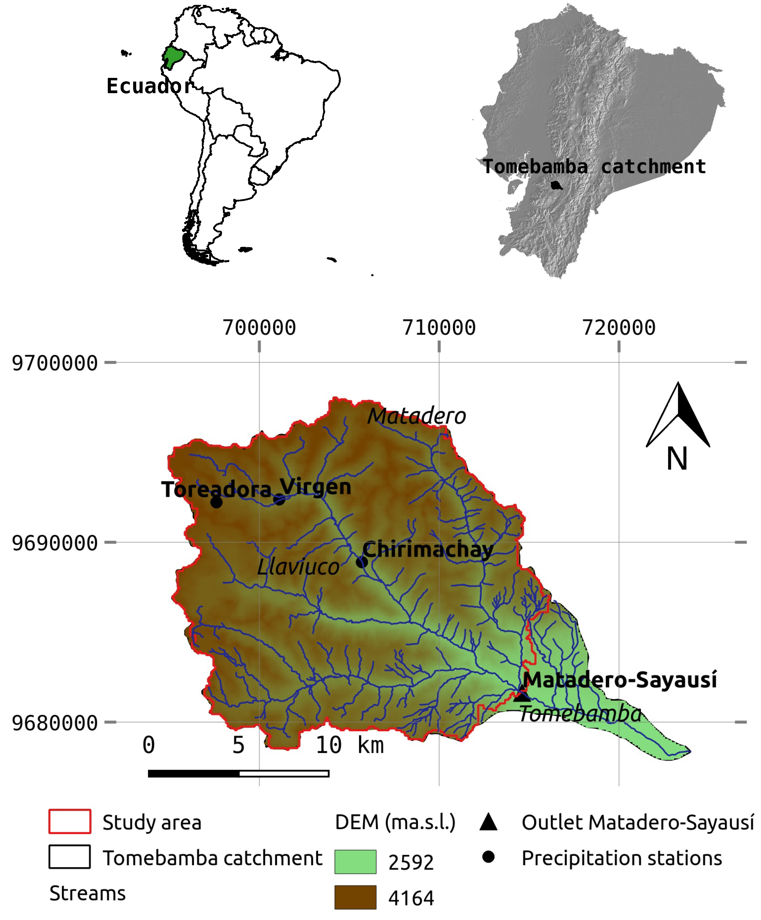
The study area is the Tomebamba catchment towards its outlet at the Matadero-Sayausí station, which corresponds mainly to a páramo ecosystem located in the south-eastern flank of the Andean cordillera of Ecuador (Figure 1). The Tomebamba catchment is part of the Cajas National Park, which was declared by UNESCO as a World Biosphere Reserve in 2013. Elevation of the study area ranges from 2800 to 4100 m above the sea level (m.a.s.l.), and covers an approximate area of 300 km${}^2$. It drains to the upper part of the Tomebamba river (area of the catchment $\approx 332$ km${}^2$), and lately to the Amazon river towards the Atlantic Ocean. The importance of the catchment is related to its water supplier role for domestic, agricultural and industrial purposes for the city of Cuenca (third largest city in Ecuador with more than 580,000 inhabitants), and even for hydro-power generation in the region.

Climate at the Tomebamba catchment is governed by continental air masses from the Amazon river basin, by the seasonal shift of the Inter Tropical Convergence Zone (ITCZ), and by the cold water upwelling of the Humboldt ocean current. As a result, convective and orographic cloud formations occurs [31]. Although precipitation (in terms of volume) mainly falls as drizzle (≈1 mm/h), higher intensity events are also experienced in the catchment (up to 140 mm/h) [32,33].

According to the classification system of the Food and Agriculture Organization (FAO) of the United Nations [34], the prevailing soil types in the Tomebamba catchment are andosol and histosols. Furthermore, studies by [35,36] in a comparable Andean micro-catchment have revealed the dominance of interflow as the major contributor to runoff generation. This is due to the inner soil properties of water storage (andosols) and organic matter content (histosols) together with the presence of wetlands and the slope of the catchment. As a result, flash-flood events are not exclusively caused by extreme precipitation events. Non-extreme precipitation events can trigger flash-floods when the soil is saturated due to the high retention capacity of the catchment. High flows are explained by the presence of histosols, whereas in contrast, low flows generation is controlled by the slope of the catchment.

Lack of spatial information describing the main flash-flood driving forces in the region limited the variables to be used as inputs to punctual measurements (time series) of precipitation and discharge. Data comprises precipitation and runoff hourly time series for a period of 2.5 years (from January 2015 to July 2017). To account for the variability of precipitation in the catchment, precipitation time series were obtained from 3 tipping-bucket rain gauge stations (Toreadora at 3955, Virgen at 3626 and Chirimachay at 3298 m.a.s.l.), which were installed within the catchment and along its altitudinal gradient. On the other hand, discharge time series were obtained for the outlet of the study catchment, at the Matadero-Sayausí station (2693 m.a.s.l.), for which the corresponding drainage area was delineated (Figure 1).

The length of the study period was further divided for training (from January 2015 to July 2016) and validation (from July 2016 to July 2017) purposes. Mean annual precipitation volumes for the study period were 1109, 1021 and 909 mm for Chirimachay, Toreadora and Virgen stations, respectively.

Figure 2 shows the precipitation (average of 3 stations) and the discharge hourly time series for the study period. An analysis of historical discharge extreme high events in the Tomebamba catchment (from 1997 to 2017) together with local media reports from the last decade served to determine a threshold value of 50 m${}^3$/s as an indicator of a dangerous event affecting the everyday life of the community and usually leading to a flood event in the catchment. This reference value has a return period of 4 months (calculated with WETSPRO, using peak-over-threshold values, see [37]). For the study period, 12 independent events were above this threshold value.

3. RF Technique

RF is a supervised ML algorithm that ensembles multiple decorrelated DTs [20]. A decision tree is a stochastic model that relates a response/outcome to explanatory variables or features. Each decision tree can be seen as a set of conditions, hierarchically organized, and successively applied to a dataset. Decorrelation among trees is assured by growing trees from different randomly resampled training sets (bagging technique) from the original dataset [22]. For regression applications, multiple DTs provide independent numerical predictions of the phenomenon of interest (i.e., discharge), contrary to class labels for classification. At the end, the outcome corresponds to the mean prediction of all individual trees.

Starting from the root (parent) node of a tree, and at every node, data is recursively partitioned into two self-similar child nodes by following simple rules related to the data and until a specified stop condition is reached [38]. To split a node, a random selection of features is used by the RF algorithm (instead of using all features). For this, a random component is used to resample and to select the optimal successive directions (features) for splitting the data with the purpose to obtain purer nodes than the parent. By minimizing node impurity, the collection of outcomes of a tree is the most homogeneous possible. Every terminal node comprises a simple regression model that applies in that node only. A detailed description of the method can be found in [20].

Strengths of the RF algorithm are related to its simplicity due the few parameters that need to be tuned, higher accuracy when compared to other ML techniques, and robustness as result of a bagging process [20]. It is capable of dealing with small size samples, high-dimensional spaces, and complex data structures [23]. The RF algorithm was used by means of the scikit-learn package for ML in Python^® [39]. The main functions, attributes and methods employed can be found in http://scikit-learn.org.

3.1. Algorithm

The RF algorithm for regression applications is as follows:

(i)

Construct each one of the decision tree models based on a random selection of a number of bootstrap samples (n_ estimators parameter) drawn with (or without) replacement from the training dataset. Each bootstrap is composed by a different subset (roughly two-thirds) of the dataset, in a process known as out-of-bag (OOB) [19]. The OBB technique aims to get unbiased estimates of the regression as well as to get estimates of the importance of the variables used for the tree construction process [40].

(ii)

Determine a number of features (max_ features parameter) to perform the best split decision from the total number of predictor variables of the dataset (n_ features). The condition max_ features < n_ features ensures the nonexistence of duplicated DTs in the forest. Consequently, by assuring variety, the problem of over-fitting is avoided. Ref. [20] recommends $max\_features=\sqrt{\mathit{n}\_\mathit{features}}$, for regression problems.

(iii)

Split each node of each decision tree into two descendant nodes by using the best split criteria. The calculation of the best splits are chosen based on the mean squared error ($MSE$) for regression problems. The minimum number of samples required to split a node is controlled by the min_ samples_ split parameter.

(iv)

Grow n_ trees as much as possible (largest extent) by repeating steps 1 to 3 until a number of nodes have been reached. The optimal number of trees is reached when the $OO{B}_{error}$ stops decreasing. The depth of each tree is controlled by the max_ depth and the min_ samples_ leaf parameters; where min_ samples_ leaf is the minimum number of samples required to be at a leaf node. This is aimed to reduce the structural complexity of the models in what is called pruning criteria [22].

(v)

Determine the prediction as the mean response from all regression trees [20].

3.2. Determination of Model Hyper-Parameters

Before using the RF algorithm, its model hyper-parameters, which basically control the structure and level of randomness of the forest [41], must be defined. For this, a random grid-search procedure was implemented to determine the optimal hyper-parameters for each model that will be built up. It consists on the assessment of the model residual mean for different combinations of the hyper-parameters on the training dataset. For this, a 3-fold cross-validation was performed to avoid overfitting. The training data was split into 3 folds; the model was iteratively fitted on the 2 folds and evaluated on the third one.

Table 1. Grid of the hyper-parameters used for a 3-fold cross-validation.

Hyper-Parameter	Values
n_estimators *	50–700
max_features	’auto’, ‘sqrt’ and ‘log2’
min_samples_split	2, 5 and 10
min_samples_leaf	1, 2 and 4
max_depth *	10–700

* Increment of 10 units.

shows the ranges of the different values of the most important hyper-parameters (according to [39]) that were evaluated. From those hyper-parameters, $n\_estimators$ and $max\_features$ are generally agreed as the most important ones during calibration (significant impact on error rate) [19,27].

3.3. Input Data Composition

The determination of the optimal model input plays a key role in model performance since it provides the basic information about the system [29]. For a precipitation-runoff forecasting model, the input coming from precipitation at the current time alone is not sufficient for the model to perform adequately. Therefore, additional information can be derived from previous time steps of precipitation and discharge. Nevertheless, an autoregressive exogenous analysis is necessary to determine the number of lags (features) of precipitation and discharge that have a significant influence on the predicted flow.

Physically, the addition of precipitation lags aims to mimic the antecedent soil moisture conditions of the catchment, which might play a key role in flash-flood forecasting (humid regions). It accounts for the fact that during dry periods, the soil is below field capacity, and therefore, it needs additional rain water first to reach field capacity and then to generate discharge. Conversely, during wet periods, the soil is at or above field capacity and needs less water to generate discharge. As a result, simulations of runoff for dry and wet periods are characterized by underestimation and overestimation of discharge, respectively [42].

To determine the number of lags to be used, [43] proposed a qualitative analysis that relies on statistical properties such as cross-, auto- and partial-auto-correlation of the data series. This method avoids a long trial-and-error-procedure when identifying the optimal composition of the input. For discharge, the autocorrelation function (ACF) and the partial autocorrelation function (PACF) with 95% confidence levels can suggest the influencing antecedent flow patterns in the discharge at a given time [6,43,44].

For precipitation, the number of regressors can be determined either through a Pearson cross-correlation applied to the data series [43], or according to the concentration time of the catchment [44]. The above input selection procedure relies on the linear relationship between the variables; however, the effect of an additional variable is not assessed.

4. Model Evaluation

Model performance or efficiency was determined by comparing the model outputs and the observed time series. For this, goodness-of-fit statistics and graphical interpretation techniques were applied together since both approaches complement each other. The shortcoming of applying only goodness-of-fit statistics is that they restrict the model assessment by representing the mean performance of the model without considering the unbalanced influence of outliers and/or extreme high (floods) or low (droughts) values [37].

4.1. Goodness-of-Fit Statistics

Model residual mean ($ME$) measures the average systematic difference between simulated and observed values. In contrast, the model residual variance ($S_{EQ}^2$) measures the average random differences. For high number of observations, the $MSE$ equals approximately the sum of the squared model residual mean and the model residual variance. As a result, the $MSE$ comprises a systematic (bias in the model) and random component (after bias correction) [37].

The disadvantage of using $MSE$, $S_{EQ}^2$ and $ME$ is their high dependence on the magnitude of variable of interest (i.e., discharge). Thus, the coefficient of efficiency also named the Nash-Sutcliffe model efficiency ($NSE$), which is less sensitive to high extreme values [45], was applied to measure the overall model accuracy. The $NSE$ is a dimensionless and scaled version of the $MSE$; it is the fraction of variability in the observations explained by the model, and it can be calculated as follows:

$$NSE=\left[1-\frac{{\sum }_{i=1}^n{\left(Q_m(i)-Q_o(i)\right)}^2}{{\sum }_{i=1}^n{\left(Q_o(i)-\overline{Q_o}\right)}^2}\right]=\left[1-\frac{MSE}{S_{Q_o}^2}\right]$$

(1)

where $Q_o$ is the mean observations value. The $NSE$ ranges between −∞ and $1.0$, being $NSE=1$ the optimal value.

The systematic error, which is the objective function, can be minimized through calibration. On the contrary, the random component cannot be removed since it is related to the inherent stochastic nature of the inputs.

Although ideal, the use of target functions designed for extreme high flows such as the mean peak difference (see [46]) was not possible due to the relatively small dataset available for the study catchment. The reason is the poor training of the trees in the forest when the objective function if specialized in extreme high values. Therefore, to use target functions larger datasets are required to capture a more complete spectrum of extreme events. Nonetheless, a solution to this issue relied in training the model for all flows, enriching the input of the model with additional information specifically aimed to improve the prediction of extreme high flows, and then assessing the efficiency of the model via means of graphical analyses focused on extreme high values (floods).

Graphical Analysis

The need to perform a more complete evaluation of model performance (analysis of extreme high values) is related to the fact that model residuals ($ME$ and $S_{E_Q}^2$) increase with higher flows. For this, a Box-Cox transformation of discharges was applied; it was calculated with the following equation:

$$Box-Cox(q)=\frac{q^{\lambda }-1}{\lambda }$$

(2)

where q is discharge and the parameter $\lambda$ can be calibrated graphically until reaching homoscedasticity in the residuals (constant standard deviation). However, according to [37], a value of lambda = 0.25 is commonly used for runoff, and thus it was adopted for this study.

Another issue related to model residuals is their common serial dependence on scales (time step) and flow magnitudes—it will be higher for shorter time steps [37]. For peak flows (floods), the serial dependence is strong for short time steps (i.e., hourly scales or smaller than the recession constant of the quickest sub-flow component). The evaluation of flows occurring at all time steps will imply a higher representativeness for low flows; therefore, the selection of nearly independent observations is necessary. Independent events were obtained by splitting the discharge time series in events and using one value per event (technique developed by [37]).

Finally, the assessment of a model under extreme conditions relied on an indirect indicator, the flow frequency distribution for extreme high values. The analysis focused on the behavior of the distribution towards the tail (i.e., higher values for peak frequency distribution). A comparison of discharge values with a visual inspection of the shape of the tail for both historical observations and simulations was applied to conclude whether model performance is acceptable for extreme conditions.

4.2. Feature Selection Analysis

Model parsimony was approached via a reduction of the input dimension using a procedure known as feature selection. It is aimed to shorten computation times by determining the relative importance of each of the features of the input and trimming off the less important ones. In some cases, feature selection even improves model accuracy [47]. Different techniques for feature selection are available; e.g., based on a variance sensitivity analysis, based on univariate statistical tests, recursive elimination, among others.

For this study, the variance sensitivity analysis was applied by following a simple procedure introduced by [48]. It measures the variance of the output produced by a single feature without considering interactions between features. The selection criteria rely on the fact that a relevant feature to the model will produce a higher output variance. The variance ($V_k$) produced by a single feature, and therefore, its relative importance ($R_k$) can be calculated as follows:

$$V_k=\frac{{\sum }_{j=1}^L{({\widehat{y}}_{t-k}(j)-\overline{{\widehat{y}}_{t-k}(j)})}^2}{L-1}$$

(3)

$$R_k=\frac{V_k}{{\sum }_{i=1}^m{V}_i}\times 100$$

(4)

where, ${\widehat{y}}_{t-k}$ is the model output obtained by holding all m input features at their average values except ${\widehat{y}}_{t-k}$, which varies according to the sample or time step, along the interval $j\in \{1, \dots , L\}$.

Finally, based on the $R_k$-values obtained, the selection principle was to retain a number of features accounting for at least 80 % of the total relative importance. The remaining features can be considered unimportant and therefore removed.

5. Step-Wise Methodology

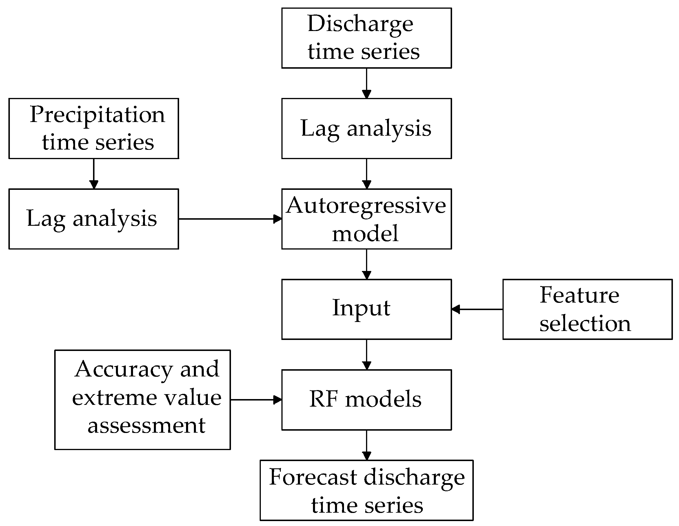
The step-wise methodology proposed in this study (Figure 3) consists in setting up several RF models to forecast discharge for a specified forecast horizon until finding the optimal or parsimonious one in terms of model efficiency. Special attention is given to the forecast of extreme high values (floods) via an analysis of their flow frequency distribution. At every step, a new model is composed by a particular input data (time series) based on the information of precipitation and discharge, and according to a lag analysis aimed to include only relevant information.

For this purpose, an autoregressive model, whose input is merely composed by discharge lags, was defined as the base model. The dimension of the input of the base model is then gradually increased by adding extra information such as precipitation observations at the current time and lags (to mimic soil moisture conditions in the catchment). Model hyper-parameters are tuned for every new model (input data composition scenario).

The outcome of the RF model is the prediction of discharge at a certain time, which lately forms a discharge time series for the specified forecast horizon. The last step, whose objective is to derive parsimonious models, is to reduce the dimension of the input based on a sensitivity analysis that determines the most relevant precipitation features accounting for the 80% of the output’s variance. The step-wise approach proposed in this study is firstly used for building up a 4-h discharge forecasting model, and later on, the arising results will serve to develop models with longer forecast horizons of varying time (8, 12, 18 and 24 h).

6. Results and Discussion

The following subsections, unless specifically mentioned, correspond to a 4-h discharge forecasting model.

6.1. Determination of the Number of Discharge and Precipitation Lags

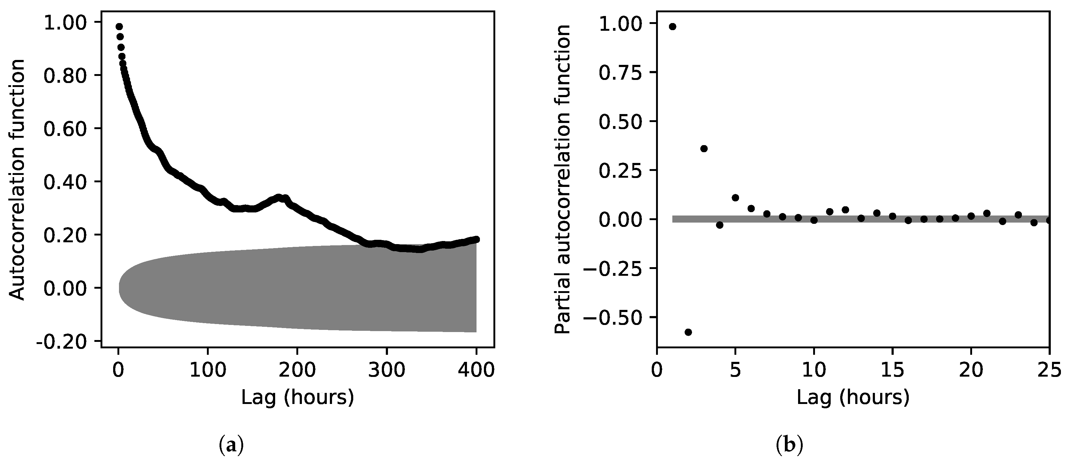
Figure 4 shows the ACF and PACF plots, respectively, from which the number of discharge lags were determined. The ACF and the corresponding 95% confidence band was estimated from lag 1 to lag 400 (h), and the highest autocorrelation occurred at the first lag. A significant correlation was revealed up to lag 300 (around 13 days). Thereafter, the correlation fell within the confidence band (Figure 4a). The systematic ACF decay demonstrated the presence of a dominant autoregressive process. Similarly, the PACF and its 95% confidence levels were estimated from lag 1 to 25. The PACF revealed a significant correlation up to lag 8. The dominance of the autoregressive process over the moving-average is proved by the rapid decay of the PACF (Figure 4b). As a result, it seemed reasonable to include discharges up to 8 lags (h) as additional inputs.

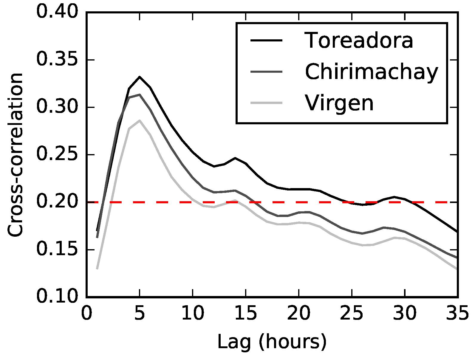
Figure 5 illustrates the Pearson’s cross-correlation between each precipitation station and the discharge time series to determine the number of precipitation lags to be used. Results revealed the highest correlation, for all stations, at lag 4 (maximum correlation of 0.3323 for Toreadora). In contrast, the concentration time of the catchment was estimated in 2.3, 3.4, 5.2 and 5.9 h according to the equations of Kirpich, Giandotti, Ven Te Chow and Temez, respectively (a summary of the equations can be found in [49]). The average concentration time (4.3 h), according to the mentioned equations, matches with the number of lags determined by the cross-correlation analysis.

6.2. Base Model: Discharge Lags as the Sole Input

The use of 8 discharge lags as the input of the base model (model A) was confirmed by a sequential process that gradually added one lag at the time until the $NSE$-values calculated for the training period stopped significantly (0.005) improving. Although the addition of more than 8 lags resulted in a slight increase of the $NSE$-values in the training period, the $NSE$-values in the validation period started deteriorating (as a result of overfitting).

Model efficiencies of the base model, whose input consisted of 8 features, obtained $NSE$-values of 0.880 and 0.652 for the training and validation periods, respectively. Moreover, according to the sensitivity analysis, the relative importance of each of the discharge lags decreased slightly and proportionally from 13.6 % (lag${}_{-1}$) to 11.6% (lag${}_{-8}$).

6.3. Precipitation Lags as Additional Inputs

To improve the base model, its input was enriched with precipitation information coming from three stations (Toreadora, Virgen and Chirimachay) from which data were available. The number of lags was determined according to the cross-correlation between each precipitation station and the discharge time series. For this, similar to [29,43], a cross-correlation threshold of 0.2 was selected, indicating that 24, 10 and 15 lags should be used for Toreadora, Virgen and Chirimachay stations, respectively.

The input of this new model (model B) was composed by precipitation information at the current time from 3 stations, their corresponding lags and discharge lags (60 features in total). Results indicated $NSE$-values of 0.954 and 0.758 for the training and validation periods, respectively.

6.4. Feature Selection

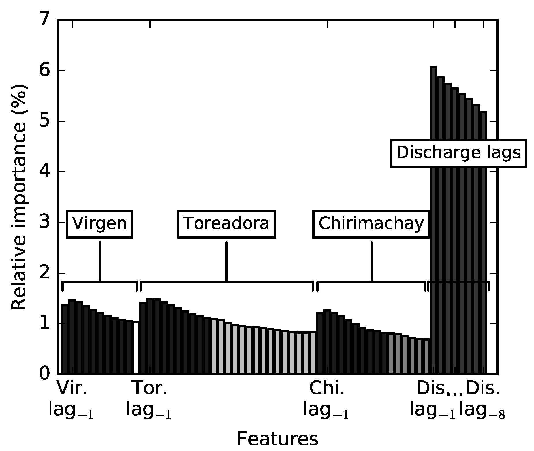
Figure 6 shows the relative importance of each of the features of model B. Results clearly show the predominance of the discharge information over precipitation. The total relative importance of the precipitation information was 44.8%. Based on the sensitivity analysis, the contribution of the three rainfall stations was 26.9, 13.5 and 14.8% for Toreadora, Virgen and Chirimachay, respectively. No relation was found between the relative importance of the precipitation station and its altitude nor distance to the outlet.

As a final stage, precipitation at the current time and 9 lags for all stations (from lag${}_{-}1$ to lag${}_{-}9$) were selected since they accounted for the 80.36 % of the total relative importance of model B. As a result, 38 features in total were used as inputs of model C (see darkest bars in Figure 6). Efficiency of model C slighted improved (0.018) when compared to model B. Results indicated $NSE$-values of 0.972 and 0.761 for the training and validation periods, respectively. 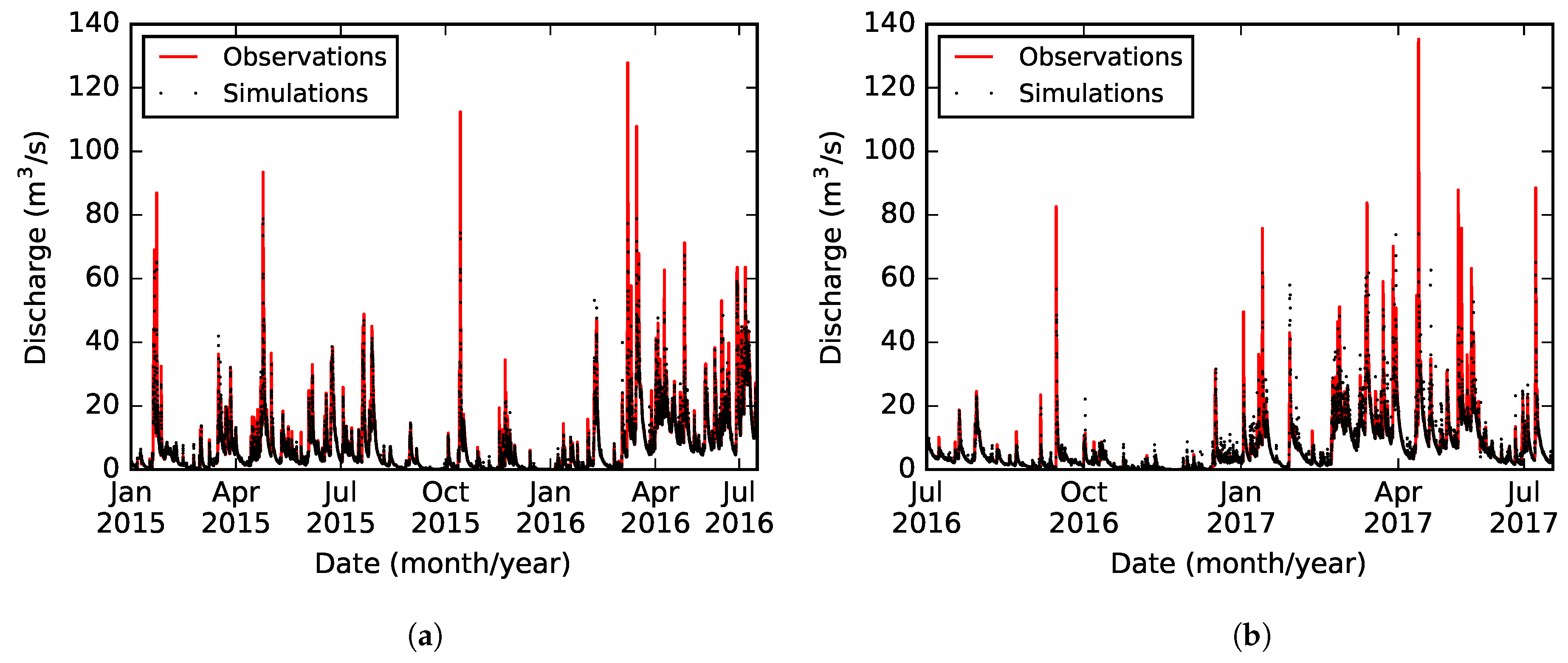Figure 7 presents the model results for both the training and validation periods. Moreover, a comparison between the results of models B and C showed a correlation coefficient ($R^2$) of 0.996. Both the slight change of model efficiencies and the comparison of results suggested that 36.7 % of the features were successfully trimmed off, achieving a parsimonious model.

In contrast, to study the usefulness of the addition of precipitation information, the lags of each station were gradually and simultaneously included in the input until reaching the best $NSE$-values for the training period. Results proved that only 4 lags per station were enough to achieve the best model performance (0.973). Results obtained $NSE$-values of 0.973 and 0.764 for the training and validation periods, respectively. Only an improvement of 0.001 of efficiency (training period) was obtained when compared to model C. Thus, the criteria of including precipitation information until reaching the 80% of the relative importance was confirmed.

6.5. Graphical Analysis

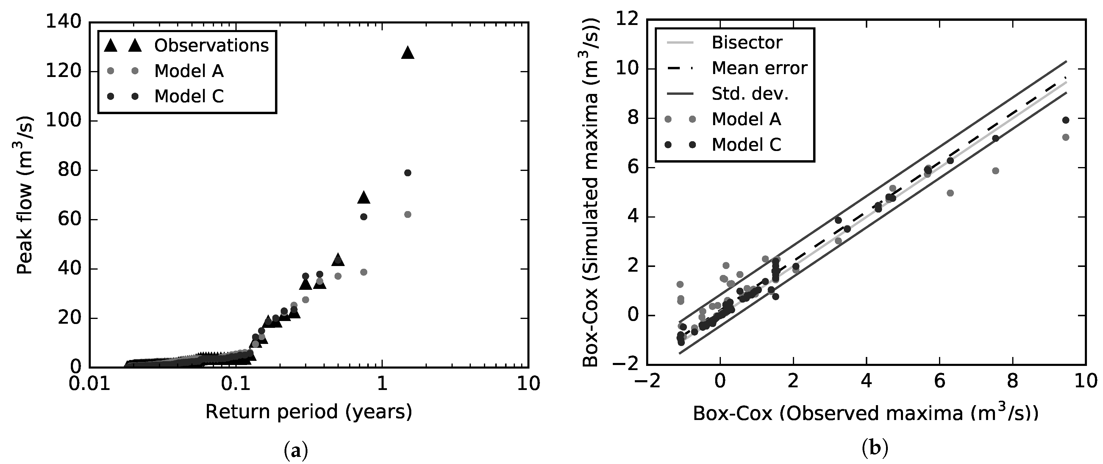
To complement goodness-of-fit statistics, Figure 8a shows the empirical extreme value distribution of peak flows for both observations and simulations (models A and C). The use of a pure autoregressive process (model A) underestimated systematically, to a greater degree, peak flows for 0.3-year return period onwards when compared to model C.

Additionally, Figure 8b shows the correlation between the predictions of models A and C (vertical axis) and the observed flows (horizontal axis) for high flows. The mean error and the standard deviation correspond to the results of model C. Model residuals are represented by the horizontal and vertical differences between each point and the bisector line. The dependence of the standard deviation on the flow magnitude was disrupted (constant standard deviation) after applying the Box-Cox transformation with a $\lambda$-value of 0.25. Predictions of model A indicate higher scatter (higher standard deviation of peak flow deviations from the bisector line) and higher bias (systematically lower mean peak flows) when compared to model C. Consequently, peak flows were systematically more underestimated by model A than model C. The improvement in the prediction of peak flows when precipitation data were included as additional inputs is therefore evident—it is considerably more significant for extreme high values. For instance, the 4-h forecast of a particular peak discharge of 69 m${}^3$/s was improved from 39 (model A) to 61 m${}^3$/s (model C).

Overall assessment of the 4-h forecasting model indicates a good match between observations and simulations for flows up to 60 m${}^3$/s (being 7.1 m${}^3$/s the mean discharge of the time series). This confirms the validity of the derived model for the forecasting of discharges historically indicating floods in the catchment (threshold value of 50 m${}^3$/s). The fact that flows above this threshold were correctly simulated determined the sufficiency of 2.5 years for calibration/validation when the objective is to provide an alarm indicating a flood risk in the catchment.

6.6. Forecasting Models of 8, 12, 18 and 24 h

The step-wise methodology applied for building up a 4-h forecasting model was further tested for longer prediction horizons of 8, 12, 18 and 24 h.

Table 2. Input data composition and model efficiencies for forecasting models and their parsimonious versions for prediction horizons of 4, 8, 12, 18 and 24 h.

Forecast Horizon	Discharge	Toreadora	Virgen	Chirimachay	Total	NSE	NSE
[h]	Lags	Lags	Lags	Lags	Features	Training	Validation
4	8	24	10	15	60	0.954	0.758
4 *	8	9	9	9	38	0.972	0.761
8	8	32	19	23	85	0.868	0.581
8 *	8	15	15	15	56	0.867	0.580
12	8	36	23	27	98	0.828	0.506
12 *	8	18	18	18	65	0.829	0.503
18	8	42	29	33	115	0.772	0.442
18 *	8	21	21	21	74	0.771	0.439
24	15	48	35	39	140	0.772	0.385
24 *	15	21	21	21	81	0.767	0.384

* Parsimonious version.

resumes their corresponding input compositions, which show that the input dimension of the best model increased (precipitation lags) accordingly to the increase of the forecast horizon analyzed. More than 8 discharge lags were only needed for the 24-h forecasting model.

Feature selection based on the variance analysis was successfully performed for all forecasting models when a fixed cross-correlation threshold of 0.2 and a target of cumulative 80 % of relative importance were used for all forecast horizons. The percentage of reduction of features without compromising model performance were 36.7, 34.1, 33.7, 35.7 and 42.1% for forecasting models of 4, 8, 12, 18 and 24 h, respectively. Additionally, a comparison between model results of the full and optimal models showed correlation coefficients ($R^2$) of 0.985, 0.996, 0.996, and 0.997 for forecast horizons of 8, 12, 18 and 24 h.

Model efficiencies in terms of $NSE$-values for the training and validation periods are shown in Table 2. Results proved that the ability of a model to forecast discharge decreases as the forecast horizon increases. Regarding the effectiveness of the feature selection analysis, only a slight change (maximum 0.003) was observed in the $NSE$-values for the validation period; in some cases feature selection improved model efficiencies.

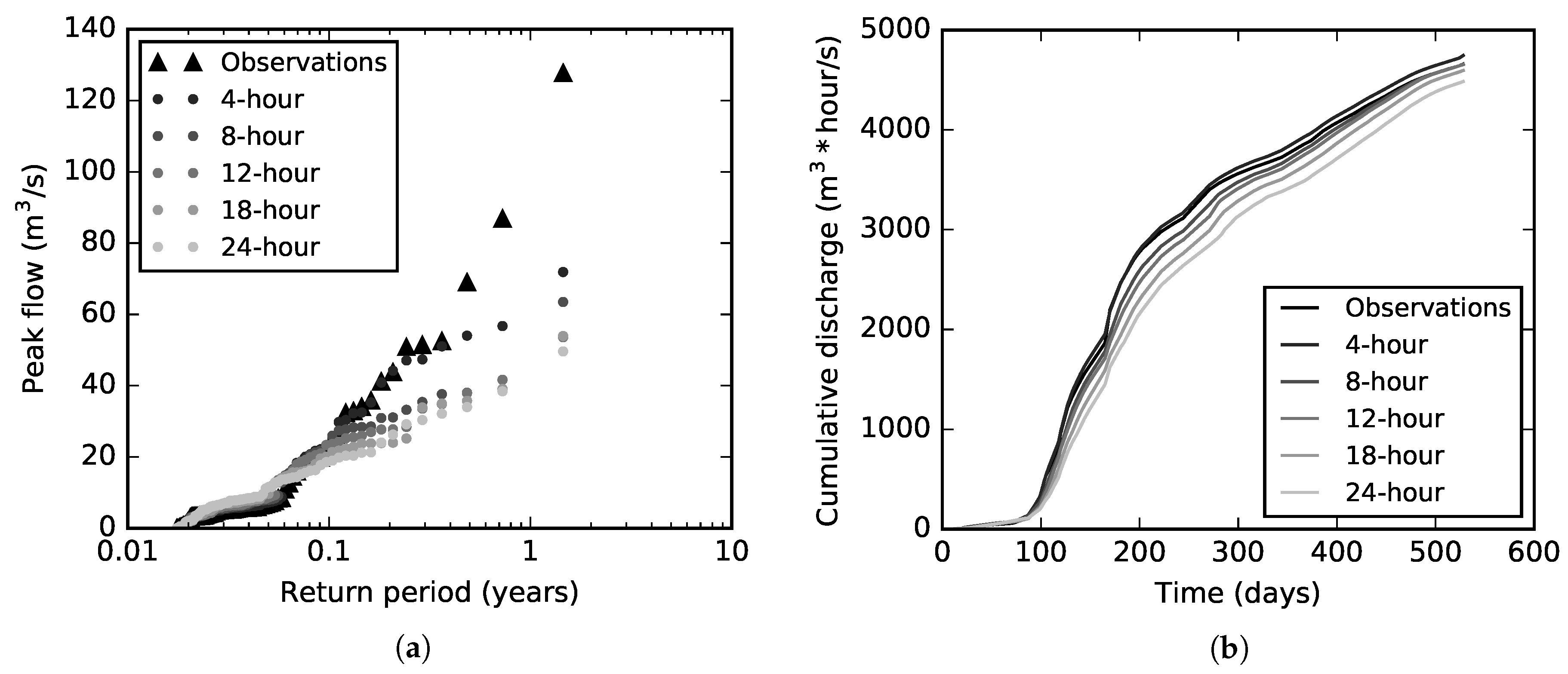
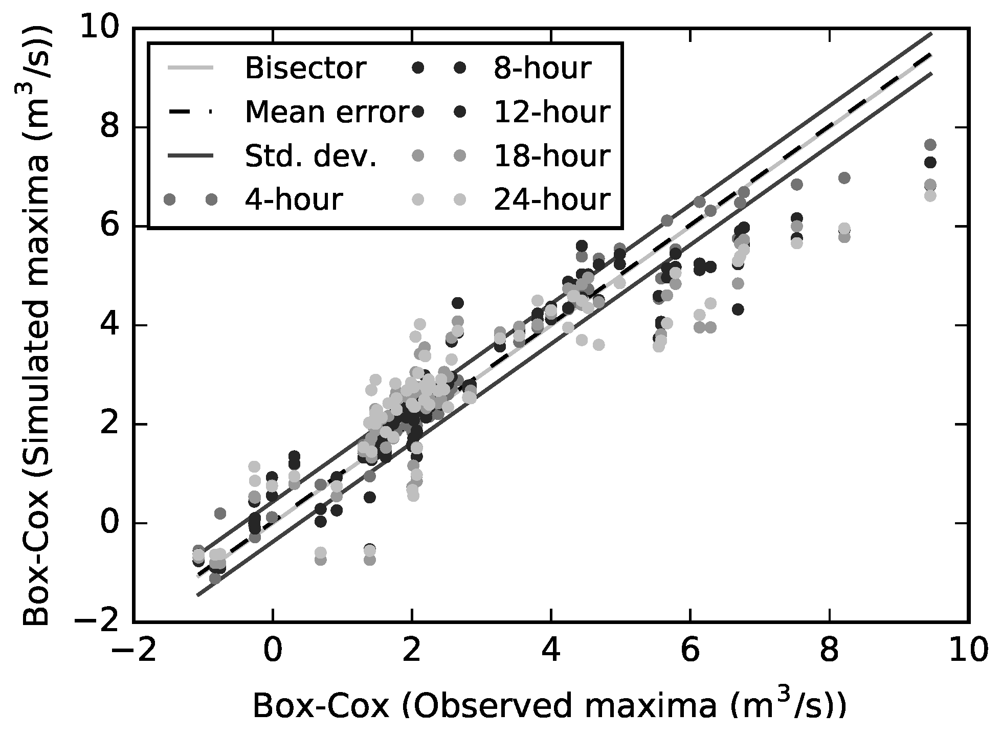
Figure 9a compares the empirical peak flow extreme value distribution of all forecast horizons (4, 8, 12, 18 and 24 h) for both observations and simulations. Only the optimal models were used for this analysis. The underestimation of extreme values towards the upper tail of the distribution became stronger as the forecast horizon increased. The lower bias of shorter forecast horizons in the empirical distribution is also reflected in the cumulative hydrograph volume (Figure 9b).

Similarly, Figure 10 shows higher scatter and bias for longer forecast horizons, which resulted in higher forecast errors when the forecast horizon increased. Strong discharge underestimations (up to 300% for the 24-h forecasting model) are explained by the simplicity of precipitation-runoff forecasting models, which lack of relevant information describing the flash-flood generation process in mountainous areas. Particularly, in páramo ecosystems, disregard of directly measured soil moisture information limits the forecasting of extreme high and low flows. As a result, the problem of underestimation of low flows and overestimation of high flows was observed in the peak flow empirical extreme value distribution.

Another factor that compromises the forecasting of extreme high flows is the insufficient representation of the spatial variability of precipitation in the catchment with only three rain gauges stations. Precipitation events might occur in areas out of the coverage of rain gauges, specifically, rain formation processes that are driven by local topography.

Besides the lack of relevant information feeding the models, the use of a relatively small dataset (2.5 years) for training and validation might also reduce the ability of the RF models to forecast discharge. This is due to the incomplete spectrum of discharge magnitudes captured by a small dataset, specially when extreme high flows are of interest. As a result, the RF models will not perform well for data points beyond the scope of the training dataset due to the average of the results of each tree in the forest and as well as the rules established for partitioning data during the training process. Results of the combined effect of the lack of relevant information and the dataset limitation can be also seen in Figure 9a, where higher errors were found for longer forecast horizons.

7. Conclusions

The development of an adequate runoff and flash-flood forecasting model is needed due to the susceptibility of lowland areas to the catastrophic socio-economic impacts of flash-floods. However, the development of such model is a complex procedure that deals with non-linear stream flow generation processes. Specifically, the use of precipitation-runoff forecasting models is targeted, as an efficient solution, for regions with lack of key-spatial information explaining the flash-flood generation process. When a model is approached through ML techniques, small datasets, high dimensionality and the difficulty to identify the importance of input features limit the proper construction of a model, and consequently, model performance optimization. Hence, to account for this issues, the use of RF models was proposed in this study to assess short-term discharge forecasting models of varying duration time (4, 8, 12, 18 and 24 h) for a mountainous region with data limitation issues.

The methodology proposed in this study have improved the current knowledge of the precipitation-runoff relations in terms of prediction over a catchment located at a high altitude. The RF ability to predict extreme values decreased as the forecast horizon increased according to goodness-of-fit statistics together with graphical analysis. Additionally, an extreme value analysis served to prove the improvement in the prediction of extreme peak values as a result of the addition of precipitation information to pure autoregressive models.

Input dimensionality reduction, applied through a feature selection method based on a sensitivity analysis, was performed for all forecasting scenarios by retaining the features accounting for 80% of the model’s variance. Significant correlation coefficients between the model results of the full and its parsimonious version, and a slight difference in NSE-values proved that the selection of the most important features was successfully achieved. Feature selection aimed to reduce the complexity of the model and to identify the processes involved in discharge prediction. At the same time, computation times were optimized.

The approach hereby proposed have the potential to be applied in different catchments sizes; however, a maximum extension of around 1000 km${}^2$ is suggested. This value intends to cover all the catchments associated with an Andean community. For larger catchments, the use of spatial information is encouraged since other relevant factors to the flash-flood generation process (e.g., topography, soil types and land uses) can be correctly represented by the most common remote sensing products. This is not the case for the Andean region, where only exceptionally fine detail, which is not feasible to obtain, would improve the model performance of RF models.

Emerging advances in ML techniques, specifically the use of the RF algorithm, have shown to serve as a powerful tool in short-term runoff forecasting. However, the use of the RF technique has been hardly documented on flood hazard assessment and particularly flash-flood forecasting. Further exploration of this technique for flash flood forecasting is therefore encouraged. Expansion of the rain gauge network or the inclusion of remote sensing imagery together with ground validation is suggested to improve the representativeness of precipitation in mountain catchments. Likewise, addition of soil moisture measurements is proposed for enriching the model to further evaluation.