North Sea Ecosystem-Scale Model-Based Quantification of Net Primary Productivity Changes by the Benthic Filter Feeder Mytilus edulis


Helmholtz-Zentrum Geesthacht, Max-Planck-Str. 1, 21502 Geesthacht, Germany
Water 2018, 10(11), 1527; https://doi.org/10.3390/w10111527
Submission received: 6 July 2018
/
Revised: 20 October 2018
/
Accepted: 22 October 2018
/
Published: 26 October 2018
(This article belongs to the Special Issue Study of Lagoons and Other Shallow Water Bodies Through the Application of Numerical Models)
Abstract
:Blue mussels are among the most abundant bivalves in shallow water along the German coasts. As filter feeders, a major ecosystem service they provide is water filtration and the vertical transfer of suspended organic and attached inorganic material to the sea floor. Laboratory and field studies previously demonstrated that blue mussels can remove large quantities of plankton from the surrounding water. I here perform numerical experiments that investigate the effect of filtration at the scale of an entire coastal sea—the southern North Sea. These experiments were performed with a state-of-the-art bentho-pelagic coupled hydrodynamic and ecosystem model and used a novel reconstruction of the benthic biomass distribution of blue mussels. The filtration effect was assessed as the simulated change in net primary productivity caused by blue mussels. In shallow water, filtration takes out up to half of the entire annual primary productivity; it is negligible in offshore waters. For the entire basin, the filtration effect is 10%. While many ecosystem models have a global parameterization for filter feeders, the coastal gradient in the filtration effect is usually not considered; our research demonstrates the importance of including spatially heterogeneous filtration in coupled bentho-pelagic ecosystem models if we want to better understand the spatial patterns in shallow water coastal systems.
1. Introduction
Blue mussels are among the most abundant bivalves in shallow water along the German coasts, both in the North Sea as well as in the Western Baltic Sea [1]. They are not only important as food for birds and fish, but also for human food culture and societal perception of the coast [2]. As filter feeders, a major ecosystem service they provide is water filtration and the vertical transfer of suspended organic and attached inorganic material to the sea floor [3]. Research interest in blue mussels, as demonstrated by a Scopus literature search (with key “Mytilus edulis”, key in title/abstract/keywords, only articles, limited to subject areas agriculture, environment, Earth sciences) goes back over a century and had a pronounced peak in the 1990s, along with a maximum in wild catch of blue mussels [4]; recently, renewed interest in blue mussels and filtration services has arisen from the major build-up of new habitats on offshore wind farm support structures [5], as contributors to and possible mitigators of water clarity for European water quality targets [6], or as a sentinel organism to indicate toxin and heavy metal concentrations [7].
Blue mussels feed on suspended material by creating an inhalant jet that passes ambient water over the gills and labial palps, where selection and compaction takes place. Intermittently, unusable material is ejected as pseudofaeces. Typical clearance rates of blue mussels measured in the lab and in the field are on the order of 1 L h−1 for one individual [8,9]. With a typical near-shore abundance of 2 m−2 the equivalent of the entire water column is thus filtered several times per year by this species alone. Measurements showed that mussels can filter approximately 20% of the biomass in a stream of water passing over a mussel farm plot of 50 ha area [10]. An extremely high clearance rate was observed over a mussel bed off the island of Sylt [9]: the entire body of water over a mussel bed passed the filtration apparatus every few hours.
Laboratory experiments have shown that the removal rate of organic material, i.e., the filtration rate, is largely proportional to the available ambient food concentration; it is on the order of 1% of mussel biomass per hour [11]. Other factors like food quality (measured, e.g., as fraction of fresh organic material or as nitrogen (N) to carbon (C) ratio), current speed, prey size, or temperature influenced the filtration rate much less [11,12,13]. At very low and very high ambient food concentrations, however, filtration is physiologically regulated: When food is scarce, mussels close their valves to avoid energy loss [14], when food is in oversupply, handling time for food items is likely to limit ingestion [15].
Mussels filter all major components of the pelagic food web. Above a mussel bed, not only the concentrations of phytoplankton are changed, but also those of bacteria, protozoa, meroplankton, and copepods [16]. Of the zooplankton, mussels consumed preferentially smaller and slow moving species [13]. Mussels have also been suggested to increase nutrient recycling by dissolved inorganic nitrogen excretion [17,18]. All of these effects, but foremost the consumption of phytoplankton biomass, influence the phytoplankton stock, the pelagic chlorophyll concentration, and eventually the annual net primary productivity (NPP, throughout this manuscript the term “productivity” shall refer to net primary productivity specifically).
Here, I perform numerical simulations with a state-of-the-art coupled bentho-pelagic ecosystem model for the shallow southern North Sea. The simulation region largely overlaps with the International Council for the Exploration of the Seas (ICES) regions 4b and 4c definition of greater North Sea ecoregions [19]. Typical productivity in this high-productivity sea is 200 mg m−2 a−1 [20]. I compare the simulated surface chlorophyll a concentrations to satellite and in situ observations for the period 2003 to 2013 and I compare the simulated productivity to results from other ecosystem model simulations and field experiments that have been performed for the North Sea in the last 20 years [21,22,23,24]. To quantify the effect of filtration, I assess the difference between two numerical experiments: one contains an explicit representation of filtration by Mytilus edulis and the other does not. Any difference found will thus be attributable to filtration.
2. Abundance Reconstruction, Numerical Models, and Experimental Setup
Blue mussels in German near-shore waters are usually represented by the species Mytilus edulis (L. 1758), and sometimes associated with or interbred with its sibling species Mytilus trossulus (Gould 1850) [25]. They occur in two distinct habitats, in the subtidal and in the intertidal; where they are not permanently under water, blue mussels prefer longer submergence over shorter submergence time. Along a salinity gradient, blue mussels prefer brackish water, where competition from non-bivalves is lower, and they tend to better evade predation pressure from the common red sea-star (Asterias rubens, L. 1758) in less marine environments [26]. Whereas subtidal blue mussels are a preferred food source for sea stars [27], intertidal mussels are mainly preyed upon by birds [28]. Bottom salinity in the simulated southern North Sea area is typically 28–34 PSU (Practical Salinity Units) and no physiological effect on blue mussels is to be expected [1].
In contrast to many other bivalves along the German coasts, blue mussels prefer hard substrate on which to settle, similar to the locally extinct European flat oyster (Ostrea edulis, L. 1758) and to the invasive Pacific oyster (Magallana gigas, Thunberg 1793), but each of these hard substrate bivalves prefers different ecological niches. Especially in the southern North Sea, natural hard substrate is rare; though it does occur in the form of erratic rocks, for example, in the Sylt Outer Reef. As a colony dweller, blue mussels create new hard-substrate environments by larval attachment to mussel shells or live mussels; these biogenic hard substrates are an important contribution to habitat formation in soft-bottom coastal seas [29]. Even when the blue mussels are overgrown by Pacific oysters, they can thrive in this co-habitation multi-layer bed and benefit from the mechanical protection provided by the epibiontic oysters [30]. Recently, hard substrate bivalves and especially blue mussels have established themselves as the major epistructural macrozoobenthos species on offshore wind farm support structures [31].
While intertidal mussel beds have long been precisely cartographed, as they used to be important in fisheries, are currently in the focus of holistic ecological analyses [32] and environmental assessment reporting for offshore industries, and within the protected world natural heritage area [33], the data situation is more unsatisfactory with subtidal mussels. These have been assayed by detailed scientific studies for the Dutch Wadden Sea area and they are regularly included in surveys within the German exclusive economic zone, or in restricted scientific surveying areas [34]. Beyond these locally confined study areas, more frequent and regional information comes from citizen scientists who report opportunistic observations of specimens to databases like the Global Biodiversity Information Facility (GBIF [35]). Necessarily, these reports are biased in time and space, e.g., fair weather conditions and the summer season and to easily accessible and often frequented locations.
To infer the distribution of a species in an entire coastal sea, habitat suitability mapping has been commonly applied [1,36] and provides information on the probability occurrence of a species. Whereas these habitat probability maps are useful for informing conservation ecology or fisheries, they are insufficient for quantitative ecological studies that need absolute abundance—and preferably biomass—of a species. Only few studies have been published that quantitatively reconstruct biomass for benthic species, let alone blue mussels, which are especially hard to quantify, because the preferred hard substrate habitats are avoided in bottom trawling and are more difficult to sample in directed scientific assessments.
Spatial data on the abundance and distribution of blue mussels in the North Sea were obtained from five open data repositories, (i) the Joint Nature Conservation Committee (JNCC), (ii) the Ocean Biogeographic Information System (OBIS [37]), (iii) the Archive for Marine Species and Habitats Data (DASSH), (iv) GBIF [35], and (v) the Belgian Marine Data Centre (BMDB). After cleaning the joined dataset of duplicate data, there remained 4074 count observations and 37,214 presence-only observations.
Presence-only data is not a preferred estimator for species distribution modeling, especially when there is a sampling bias. Many of the GBIF-reported blue mussel observations are opportunistic finds reported by citizen scientist divers, with a bias towards more accessible near-coast areas. This bias may be mediated by taking into account additional environmental constraints, which can serve as proximate absence [38]. It must be emphasized that the epibenthic reconstruction of blue mussel abundance presented here remains preliminary and subject to further research. I briefly discuss the sensitivity of the analysis to the reconstruction uncertainty further below.
The blue mussel prefers larger sediment grain sizes [39]; grain size has been found to be the best predictor of blue mussel abundance among all environmental factors in shallow water [40]. In addition, a depth limit has been observed, below which mussels do not frequently occur [41,42]. At depths below 10 m, we assume here a random abundance density up to 0.5 m−2 based on a compromise between field sampling data in a deep tidal channel [42] and definitive absence from areas recently sampled in the German exclusive economic zone [43].
For subtidal mussels in shallow water the presence-only habitat data and count data were related to bathymetry and sediment grain size available from the North Sea Assessment of Habitats (NOAH) atlas (www.noah-project.de/habitatatlas/). The relationship between mussel abundance and grain size constrained by bathymetry informed a Random Forest model (RF) [44] to predict the species abundance for the entire model domain [40,45]. Mussel beds were incorporated as point data using the Oslo-Paris (OSPAR) Biodiversity Committee habitat classification. Within these beds, a constant density of 3911 m−2 is assumed [16].
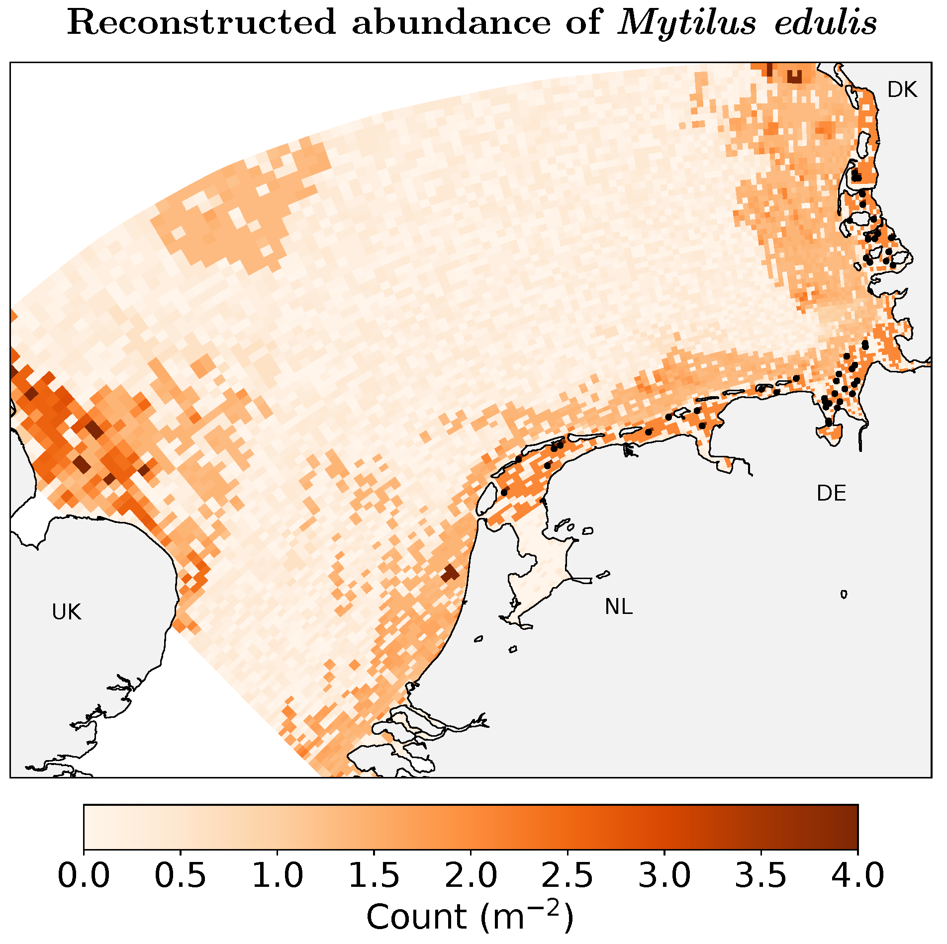
Comparison to Wadden Sea field data [40] indicated that predicted shallow-water mussel abundance was overestimated, which can be attributed to the positive sampling bias in the citizen-science data set. I thus interpreted the RF absolute abundance prediction as relative occurrence and rescaled it to laterally align with the Wadden Sea field data [40]. Furthermore, the mussel bed data were scaled according to their patchiness in the numerical grid (see below). The combination of random offshore abundance, species-distribution modelled coastal, and additional mussel bed abundance results in the reconstructed abundance shown in Figure 1.
2.1. Numerical Models
The description of interactions between pelagic and benthic compartments, and between hydrodynamics, pelagic ecology, benthic biogeochemistry, and benthic filtration requires a spatially and functionally coupled model approach, for which we employ the open source Modular System for Shelves and Coasts (MOSSCO, www.mossco.de) [46]. MOSSCO-coupled applications for the 3D coastal ocean have focussed on processes at the benthic–pelagic interface and, among others, explain spatio-temporal patterns in coastal nutrient concentration [47,48], annual net primary productivity [5], macrobenthic biomass and community dynamics [49], and suspended sediment concentration as affected by macrobenthic activities [50].
In the current coupled application, we employed the General Estuarine Transport Model (GETM) [51,52] as a hydrodynamic driver with prognostic temperature, sea level, and salinity; GETM has previously demonstrated high skill in various studies for the North Sea and the southern North Sea [53,54]. A coupling layer representing GETM in an Earth System Modeling Framework (ESMF) [55] in MOSSCO delivers interoperability of the hydrodynamics with all other components.
The Model for Adaptive Ecosystems in Coastal Seas (MAECS) [48,56] was used to describe the pelagic ecosystem; it was coupled in the MOSSCO context through the pelagic Framework for Aquatic Biogeochemistry (FABM) [57] and its ESMF component [46]; all pelagic tracers were transported by GETM. MAECS is a four-compartment nutrient–phytoplankton–zooplankton–detritus (NPZD) based model with adaptive stoichiometry following the acclimation and optimal uptake of phytoplankton cell-internal elemental quotas [56]. Multi-annual MAECS simulations have been extensively evaluated against (amongst other comparisons to ICES monitoring, satellite, and cruise observation) surface nutrient and chlorophyll station data for the decade 2000–2010 [48]. For the description of benthic biogeochemistry, a version of the Ocean Margin Experiment Diagenetic model (OMExDia) [58] with additional phosphorous cycle [47] was coupled within MOSSCO via a second ESMF component of FABM defined in the ocean floor domain.
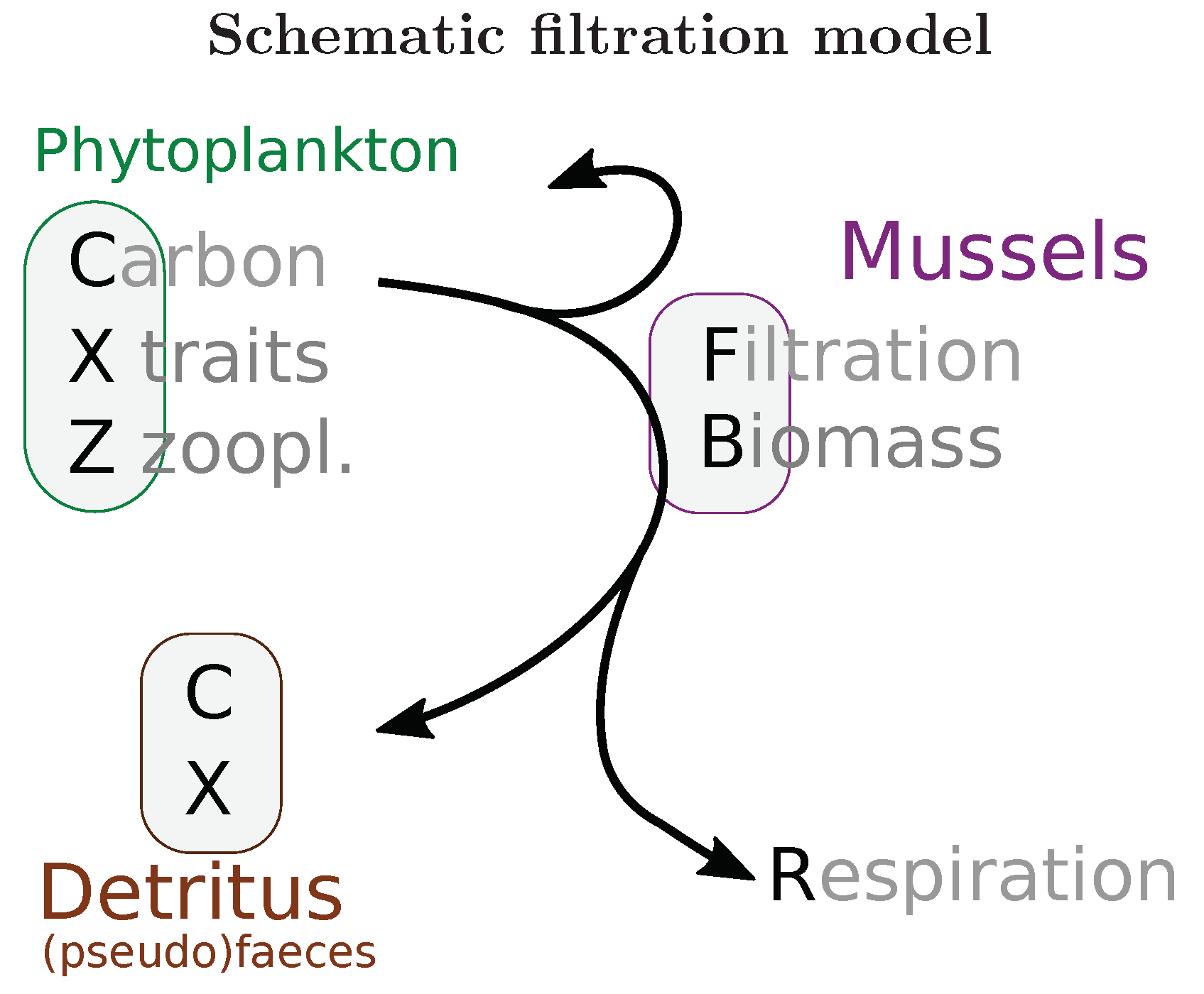
A new filtration model [5] parameterized based on lab experiments [11] was coupled as an ESMF component into the lowermost hydrodynamic layer. This benthic model removes in stoichiometric proportion particulate carbon, nitrogen, and phosphorous from the pelagic phytoplankton compartment; it considers also dependent quantities (like chlorophyll) and traits (e.g., Rubisco allocation) from MAECS. The phytoplankton compartment is converted to detritus, representing faeces and pseudofaeces, in carbon, nitrogen and phosphorous (Figure 2). A fertilization effect by nitrogen excretion has been suggested [17], but extensive sensitivity testing where nitrogen was diverted to the inorganic nutrient pool instead of the detritus pool showed no significant effect on primary production in our model setup; this direct excretion was consequently not considered in this study.
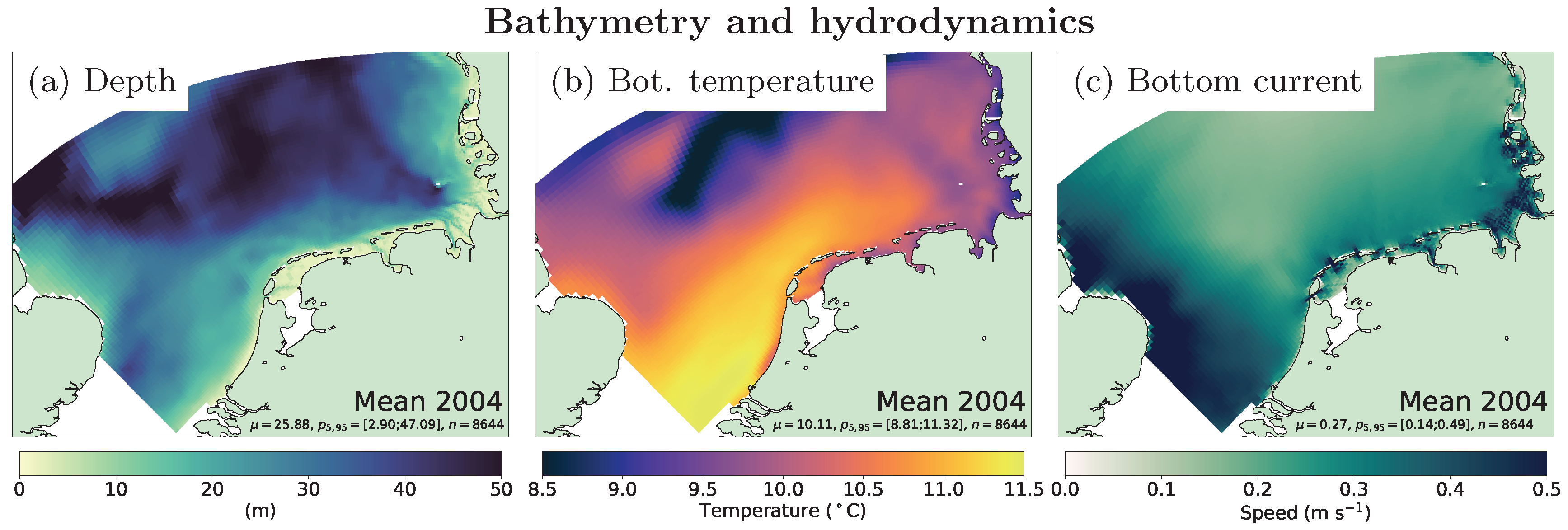
The filtration model is built around the average filtration rate (FR, the removal rate of material filtered from the water volume) of a blue mussel population. The effect of velocity-dependent clearance has been neglected in this study since the bottom current (Figure 3) usually exceeds the minimum current velocity thresholds observed [12].
No physiological regulation of filtration from high food concentration is to be expected for the natural ambient concentrations found in our model domain (below 100 mmol C m−3), and blue mussels can be expected to fully exploit their food [17]. To avoid energetic loss at low ambient food concentration, a valve closure threshold [14] was considered; all conversions were performed according to Ricciardi et al. [59]. Likewise, there is no effect of low salinity on physiology expected in our model domain.
For a single blue mussel individual, we calculate FR from phytoplankton carbon amount concentration ([C]) as FRTPM = 0.05 [C]0.983, referring to the empirical total particulate matter (TPM)–FR relationship [11] and using the following conversions: (i) carbon mass to molar with a factor of 12.011 mg mmol−1, (ii) a experimentally-determined organic matter fraction of 56%, (iii) Redfield stoichiometry to express dry weight (DW) to amount carbon ratio as 32.432 mg DW (mmol C)−1, (iv) metabolic scaling [60] with mass based on experimentally confirmed exponent 0.67 based on reference indidual DW 300 mg [11]. The lower threshold for filtration was set to 0.7 mmol C m−3 [14].
Bentho-pelagic exchanges are mediated by the specialized ESMF couplers that take care of the different representations of carbon and nitrogen in MAECS and OMExDia, and that parameterize the burial of detrital material at the sea floor [46].
2.2. Experiment Setup
The model domain was represented on a logically rectangular grid; for compromising between high resolution and numerical efficiency, the grid was reprojected with highest resolution in the Elbe estuary and lower resolution offshore, with respective cell size between 2 and 64 km2. Twenty vertical terrain-following layers were used to represent the water column, and 15 layers were used to describe the upper 20 cm of the ocean floor. Freshwater and nutrient inputs were considered for the Elbe, Ems, Weser, Scheldt, North Sea Canal, Rhine, Meuse, Humber, and Wash rivers, and for Lake Ijssel. Climatologic zero-gradient open boundary dissolved and particulate nutrient conditions were taken from a North Atlantic shelf simulation with Ecosystem Model Hamburg (ECOHAM) [61]; tides were astronomically forced at the open boundary as sea surface elevation. Air temperature and wind were taken from the the long-term Climate Limited area Model reconstruction available in the coastDat database [62].
Simulations were run for the decade 2000–2013. The first three years were discarded to avoid spin-up effects from the model initialization, which was needed to redistribute the pelagic pools of nutrients in winter. Two different scenarios were compared: (1) presence of epibenthic mussels (scenario REF), and (2) no presence of epibenthic mussels (scenario NONE).
MAECS was parameterized consistent with prior experiments [5,48], i.e., with active photo- and enzyme acclimation, phosphorous cycle, grazing and virus mortality, but without silicate and oxygen cycles. Diagnostic rates of relative carbon uptake were multiplied by phytoplankton carbon concentration and subsequently integrated over the entire year to obtain the annual net primary productivity.
The 3D time step of the hydrodynamic model was 6 min. Data exchange between the different components of the model system was performed every 30 min. The bottom roughness length was constant at 0.002 m, wave forcing was disabled. A Jerlov Type III water class was used for the radiation scheme.
2.3. Data for Model Evaluation
Observational data is by definition not available for annual net primary productivity and data on primary production is not routinely available at the scale of the southern North Sea (SNS). Chlorophyll concentration, however, is routinely observed as backscatter (“ocean colour”) or fluorescence from remote sensing and in situ instruments. Here, I evaluate the simulated chlorophyll concentration against observations collected in the European Space Agency Ocean Colour Climate Change Initiative (ESA-CCI version 3.1, [63]), a multi-platform combined remote sensing product of chlorophyll concentration. A time transgressive comparison is achieved with near-surface chlorophyll observations collected in the OpenEarth portal [64]. Comparison stations were chosen from three transects that cross the coastal gradient from the West Frisian islands Terschelling and Rottumerplate, and outward from Noordwijk. Monitoring stations along these transects are located approximately 5, 10, 15, 30, 50, and 70 km offshore, and, in addition, 235 km offshore on the Terschelling transect. Additional stations are located at the Elbe estuary and at the North Frisian coast (Figure 4 and Figure S1).
3. Results
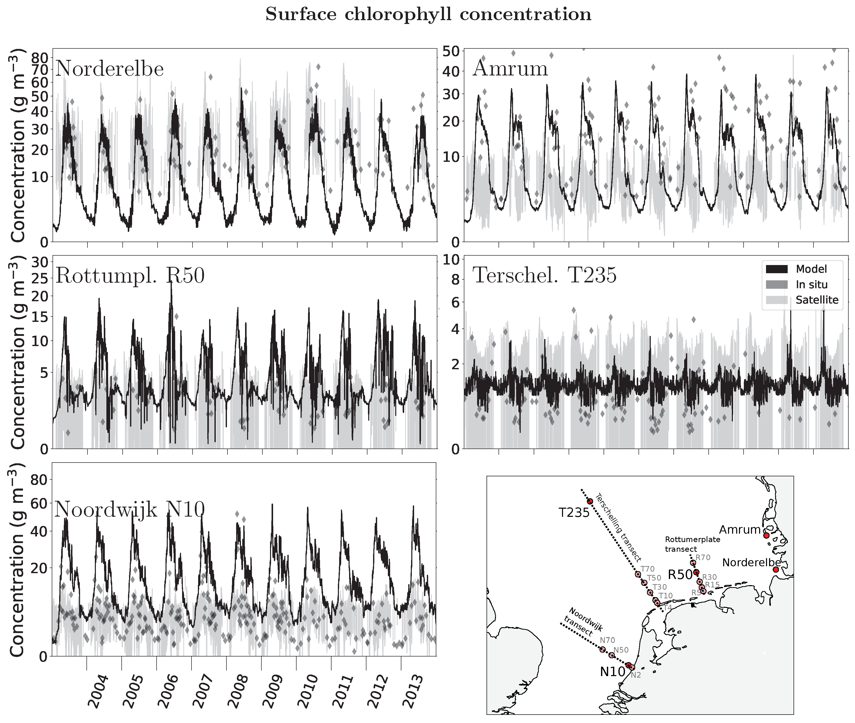
The simulated phytoplankton carbon stock assessed as surface chlorophyll concentration represents the temporal and spatial patterns observed in the decade 2003–2013. There is a pronounced seasonal cycle and interannual variability in simulated chlorophyll. Simulated chlorophyll peaks during the spring bloom at 50 mg m−3 near major river inflows (stations Norderelbe, Noordwijk 10, Figure 4). At the Norderelbe station, the 2013 late summer bloom exceeds the spring bloom, consistent with the observed unusal large nutrient input by the Elbe flood in summer 2013 [65]. At this station, the simulated variability is lower than observed (standard deviation of 11.6 versus 18.7 mg m−3, consistent with a model bias of −14 mg m−3, r = 0.32). At the other river inflow station (Noordwijk 10), model variability is higher than observed (12.2 versus 6.0 mg m−3), and the model’s bias is positive at 10.4 mg m−3.
The maximum chlorophyll concentration is smaller the more offshore the station is. At 50 km from the coast, the Rottumerplate station simulated variability is 3.8 mg m−3 (observed 2.3 mg m−3, model bias +2.3 mg m−3, r = 0.26). At 235 km from the coast, mean annual chlorophyll is down to less than 5 mg m−3 (station Terschelling 235). There, simulated and observed variability is 0.4 and 1.1 mg m−3, respectively, with a model bias of +0.2 mg m−3 (r = 0.25). Simulated minimum values of winter chlorophyll are well below 5 mg m−3 everywhere.
Observational remote sensing data as ESA-CCI Ocean Colour is available for most of the simulated period. The seasonal variability evaluated at the time series stations is in general less than the simulated variability, except for the Norderelbe station, where remotely sensed chlorophyll ranges between 10 and 60 mg m−3.
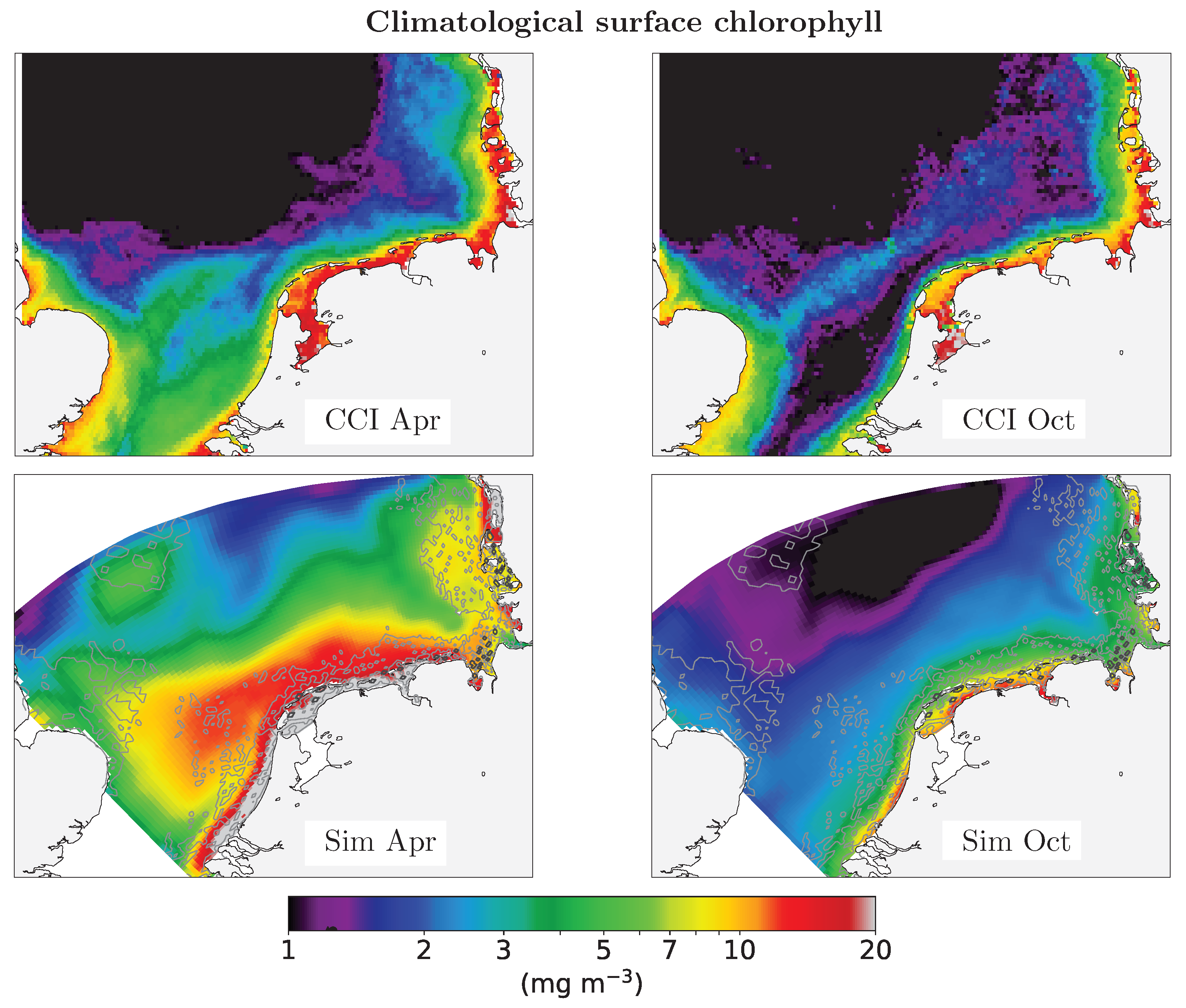
The satellite-observed distribution of climatologial spring and fall chlorophyll exhibits a strong coastal gradient with very high values (around 15 mg m−3) in a narrow band along the shore and small values offshore (≤1 mg m−3) in all seasons (Figure 5 and Figures S2–S4). The observed seasonal variability is greatest in the Southern Bight, i.e., ICES region 4c [19], and at water depths between 5 and 15 m. There is a prounced relative chlorophyll maximum in the East Anglia plume, which extends from the East Anglia coast northeast parallel to the Dutch coastline.
Simulated variability is seasonally and laterally stronger in the simulation than in the satellite observations. In April, chlorophyll concentration exceeds 20 mg m−3 in the western and eastern Frisian Wadden Sea. High surface chlorophyll concentrations (>15 mg m−3) occur not only in the Southern Bight, but in the entire southern part of the SNS. In October, coastal simulated chlorophyll concentration is in the order of 15 mg m−3; in contrast to observations, the pronounced fall minimum in the Southern Bight is not apparent in the simulation.
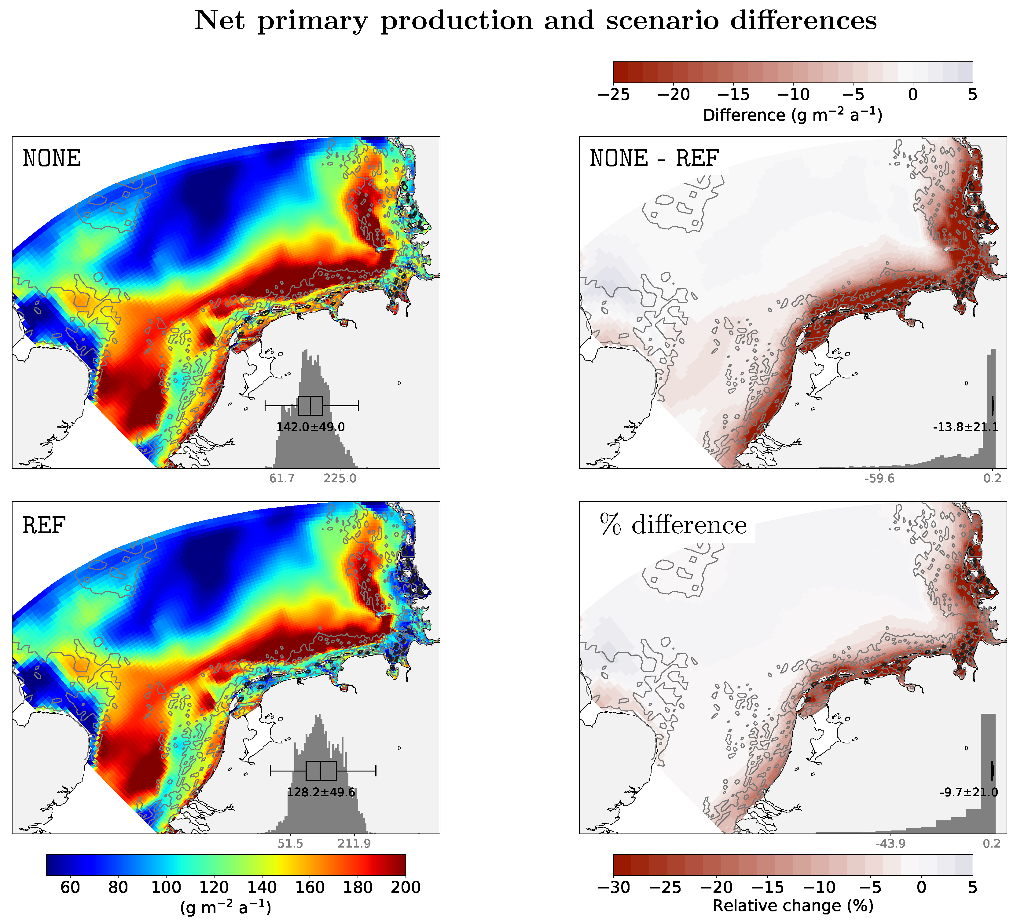
Simulated climatological net primary productivity in the SNS is 130 g m−2 a−1 (Figure 6 and Figures S5–S7). There is low productivity far offshore (50 g m−2 a−1), and productivity peaks along the 25 m depth contour along the German an Dutch coast where it exceeds 200 g m−2 a−1. Around the Frisian barrier islands, productivity is 150 g m−2 a−1 in the simulation without filtration. In the REF scenario with active filtration, productivity is decreased only around the barrier islands and is around 90 g m−2 a−1. Expressed as relative change, much of the barrier island region has a 30% lower productivity due to filtration.
4. Discussion
Simulated annual primary productivity in the southern North Sea is 142 g m−2 a−1 and covers a range of 62 to 225 g m−2 a−1 (5 and 95 percentile, n = 8686, Figure 6). This range compares favorably to one of the first coupled hydrodynamics-ecosystem model simulations [22]: a range of 90 to 200 g m−2 a−1 was estimated by their NORWegian ECOlogical Model (NORWECOM). These simulated estimates agree with in situ data presented in the NERC (Natural Environment Research Council) North Sea Report [21], who found for the western and eastern Wadden sea and the central North Sea values of 199, 261, and 119 g m−2 a−1, respectively. A lower coastal productivity was simulated by HAMSOM–ECOSMO (Hamburg Shelf Ocean Model–Ecosystem Model) for the North and Baltic Sea [23]. For the near-coast region of the southern North Sea and for the Southern Bight, they estimate an NPP of up 150 g m−2 a−1, while more offshore the productivity is around 60 g m−2 a−1. In their long-term study [66], the same model system simulates in a reference scenario for the southern North Sea NPP of 104–113 g m−2 a−1. NPP simulated with GETM and the European Regional Seas Ecosystem Model (ERSEM) [24] is much higher (on average 318 g m−2 a−1) than NPP simulated here or in most other studies. The term “SNS” used there, however, refers to a very different region: a small area within the Southern Bight (ICES area 4c). Additionally, in this simulation, I find very high productivity above 200 g m−2 a−1, but not exceeding 250 g m−2 a−1, which is also the simulated maximum along the 25 m depth contour, consistent with peak estimates for the continental coastal region of around 250 g m−2 a−1 [20,24]. These cited comparisons, summarized in Table 1, and also inter-model studies that compare many different ecosystem models for this region [67] underline that inter-model differences of NPP estimates are quite high, and that the simulations performed for this study give plausible values for NPP both in variability and absolute terms.
The difference caused by adding a filtration module to the (Figure 6) coupled system is striking in terms of magnitude: up to 40% of NPP are removed by this single filter feeder species, and 10% for the entire SNS. These high loss rates are consistent with field observations that found very high clearance of water above beds [9], or when passing through a mussel farm [10], and similar for an accompanying model study of the Firth of Thames estuary [18].
There is still a large difference between in situ and remote sensing observations of chlorophyll that are both used for parameterization or comparison of model-simulated chlorophyll [48,68] and Wirtz, K.W. (Physics or biology? Persistent chlorophyll accumulation in a shallow coastal sea explained by pathogens and carnivorous grazing, submitted manuscript, hereinafter referred to as Wirtz, submitted). As this difference between observation platforms is not uniform, Wirtz (submitted) suggested to apply an additional correction factor to the remote sensing observation such that it represents the in situ measurements better. At remote and non-river influenced stations such as along the Terschelling T50/235 or Rottumerplate R50/70 transects, remote sensing observations and in situ measurements agree, while they diverge at all Noordwijk stations, especially near the coast (N2) (Figure 4 and SOM).
It is thus not surprising that comparisons between models and remote sensing products come out unfavorable for models. Large inter-model differences aggravate the situation: Two different hydrodynamic models (GETM and NEMO, Nucleus for European Modelling of the Ocean) were both coupled to the ecosystem model ERSEM (European Regional Seas Ecosystem Model) to simulate phytoplankton community structure in the North Sea [68]. The comparison to SeaWiFS-derived remotely sensed chlorophyll shows that one model (NEMO–ERSEM) reproduces the observed mean value of chlorophyll better but lacks much of the spatial variability found in the data; their other model (GETM–ERSEM–BFM, Biogeochemical Flux Model) reproduced the high productivity region along the coast quantitatively. Its coastal gradient, however, is so strong that it underestimates chlorophyll in the central North Sea.
In this study, which employs the combination of hydrodynamics and ecosystem GETM–MAECS, the simulated mean climatological surface chlorophyll concentration is 5.2 mg m−3, and is thus about twice as much as simulated with POLCOMS–ERSEM (Proudman Oceanographic Laboratory Coastal Ocean Modelling System) [69]. GETM–MAECS chlorophyll also shows the strong coastal gradient that was simulated with GETM–ERSEM–BFM [68], and that is visible in the composite ESA-CCI Ocean Colour sensing product. GETM–MAECS represents the offshore low chlorophyll values better, but simulates much higher chlorophyll during the spring bloom and near the coast (compared to the satellite, Figure 5). A similar higher simulated than satellite-observed growing season chlorophyll was also found with GETM–MAECS in a prior study [48]. The comparison to the satellite product is therefore not suitable to assess whether the addition of filtration makes a particular simulation or coupled model constellation more realistic.
The comparison of simulated chlorophyll to the station data shows indeed that the model captures much of the observed variability and range of chlorophyll observations. At the Norderelbe station, in situ and model data align near-perfect, with a general small underestimation by the model in both spring peak and winter low (Figure 4); likewise at the Amrum station. There, however, a temporal mismatch between the simulated and observed bloom peaks is striking, with an often too early and too steeply faltering simulated phytoplankton bloom. Despite good model–station agreement, the ESA-CCI Ocean Colour comparison at the stations looks very different. There is good agreement at Norderelbe but a factor three underestimation by the model at Amrum.
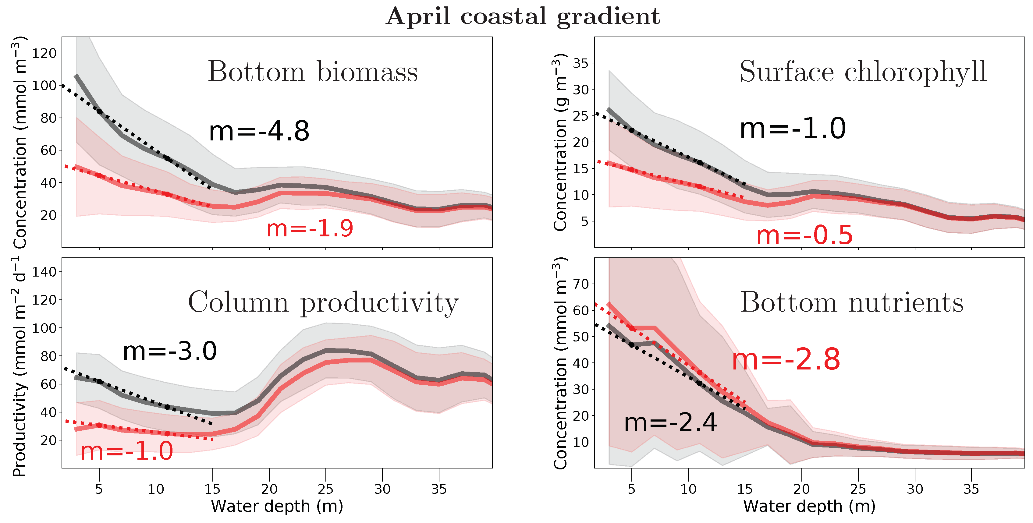
Figure 7 shows selected simulated biogeochemical quantities along the coastal gradient, i.e., for different depths intervals in a climatological April. Column productivity is between 40 and 80 mmol m−2 d−1 up to 40 m water depth. It decreases slightly over the first 15 m depth levels, together with surface chlorophyll concentration. NPP then increases strongly to peak around the 25 m depth level, consistent with the effect of more water at almost constant chlorophyll concentration. The strongest effect of filtration is the flattening of the coastal gradient: the filtration effect is largest in very shallow water and is negligible at depth greater than 30 m. The mechanism that leads to this productivity effect is the removal of near-bottom phytoplankton biomass: more than 50% of the phytoplankton stock are removed by filtration at water depths below 10 m. This bottom biomass removal results in a decrease in surface chlorophyll, but with a reduced effect. The removal of phytoplankton leads to an increase in the available nutrient concentration in April, i.e., during the bloom. These nutrients are then available for a longer, more sustained bloom. This can be seen in the model results for the summer, where the surface chlorophyll is consequently elevated compared to the the simulation without filtration. Thus, the consideration of filter-feeding reduces phytoplankton during the bloom but prolongs the bloom period by way of enhanced nutrient availability.
The current model increases the quality of ejected detritus (by respiratory removal of carbon) but does not consider a fast recycling by direct excretion of inorganic nitrogen [17,18]; filtration has no measurable effect on zooplankton during spring and summer but in the fall, where it decreases zooplankton by 20% near-shore. Both fast recycling and secondary effects of zooplankton filtration will be assessed in further studies. Clearly, however, the coastal gradient of phytoplankton stock and productivity is changed by benthic filtration.
Currently, most ecosystem models parameterize the effect of benthic filtration as one contribution to a global mortality factor (e.g., MAECS, POLCOMS, ECOSMO) and disregard the spatial heterogeneity introduced by greatly varying macrobenthic abundance and activity [32]. The explicit inclusion of benthic filtration in ecosystem models could improve the representation of the coastal gradient markedly, especially as zooplankton mortality near-shore is not sufficiently explained in current ecosystem models (Wirtz, submitted).
To help improve the understanding of the processes shaping the coastal gradient of phytoplankton, nutrients, and productivity with numerical estimates, the data base for macrobenthic stock and activity also has to be enlarged. Surveys have been institutionalized by ICES or are (ir-)regularly conducted in regional studies in the Wadden Sea, the German exclusive economic zone, or off Sylt [34,40,70]. The largest uncertainty of the quantitative estimates for the effect of filtration on ecosystem productivity is the initial reconstruction of filter feeder abundance. The sampling bias, the predominant presence/absence information, the reliance on count instead of (functionally preferred) biomass introduce uncertainty that can only be reduced by more field data.
At least the effect uncertainty can be assessed within the model context with sensitivity experiments. I chose to apply a scaling factor ranging over two orders of magnitude on the reconstructed benthic biomass distribution, and assessed the changes in annual net primary productivity in each of those experiments (Table 2). In all experiments with very low factors (scenario NONE and factors at or below 0.2) there is no effect on productivity. Near the reference factor, there is a linear increase in NPP loss in both mean and median, pointing to local rate effects in the uncertainty; the distribution of this loss is skewed (very different mean and median) and points to the observed strong coastal gradient in productivity decreases. At very high factors, the coastal NPP productivity decrease is saturated while in the more offshore regions, productivity can still be decreased by increasing filtration (median is catching up to the mean). Overall, a 10-fold increase of filtration over REF decreases NPP by 37% and 17% (mean and median, respectively.)
Mussel abundance was reconstructed for this study from opportunistic finds that are certainly biased towards fair-weather conditions. The reconstruction thus represents most likely the summer, where blue mussels have their seasonal abundance peak [31]. The reconstructed distribution is positively biased for other seasons and the filtration model does currently not account for temperature-dependent filtration activity of blue mussels. The largest filtration effect, however, also occurs during the summer season and near the coast, where and when food concentration also peaks (Figure 4, Seasonality is thus partly represented in the model.
Can we use this sensitivity to scale up from the effect of blue mussels alone to the effect of the entire benthic filtration feeding community? In the Synoptic Intertidal BEnthic Survey (SIBES) [40], blue mussels were found to constitute 6% of the total biomass of all benthic macrofauna in the Wadden Sea. They were the sixth most common species by biomass, and represent 13% of the large filter-feeding macrofauna. Total filter-feeding could consequently be assumed to amount to about eight times the filter-feeding by blue mussels, if species-specific rates are not taken into consideration. As I am using a reconstruction of the standing stock, interspecies effects such as competition is accounted for in this calculation.
As a spatial effect, the entire community filtration can be expected to be larger than the simulated filtration where blue mussels are not the dominant species, e.g., further offshore. For the near-shore areas, I expect a saturation effect when food for filter-feeding the entire community becomes limiting. By assuming as a sensitivity a spatially homogenous abundance of blue mussels in the entire model domain, I attempted to approximate total community filtration in the model. In such a sensitivity study, the gradient is regionally restored to one without filtration. Mussel beds, however, would still create large local gradients.
This remains only a very crude approximation for other species. Even if a stronger community effect should be expected over the effect of blue mussels alone, in deeper water the location of the (benthic) filter feeders is decoupled from the location of the food sources (surface layers and euphotic zone). Only with the artificially bringing of benthic life toward the surface (on support structures for wind farms, for example) can a strong effect be expected, and has been modeled [5]. It will be necessary in further studies to include the entire community with species-specific filtration rates and species-specific geographic reconstructions, or alternatively, consider functional traits of the community to improve the quantitative estimation of filtration services at the community scale.
5. Conclusions
I performed numerical experiments to quantify the effect of benthic filter feeding on the ecosystem in a coastal sea. A novel reconstruction of M. edulis abundance for the southern North Sea was created, a filtration model was added to a coupled bentho-pelagic model system including the adaptive trait ecosystem model MAECS. Over the decade 2003 to 2013, there was a pronounced effect, observed by contrasting scenarios with and without filtration on annual net primary productivity (NPP): up to 40% of NPP (locally and 10% for the entire basin) were consumed by filter feeders. While this is the first estimate of the filtration effect for a coastal sea, it is in agreement with prior small-scale estimates. Because of the strong changes and large spatial heterogeneity, I believe it is necessary to revise parameterizations for filtration in current ecosystem models to better represent the coastal gradient and advance the coupling of the benthic and pelagic domains, that still, 20 years after Arntz et al. cautioned this [71], is undervalued in coastal system modeling.
5.1. Data and Code Availability Statement
The MOSSCO software is licensed under the GNU General Public License 3.0, a copyleft open source license that allows the use, distribution and modification of the software under the same terms. All documentation for MOSSCO is licensed under the Creative Commons Attribution Share-Alike 4.0 (CC-by-SA), a copyleft open document license that allows use, distribution and modification of the documentation under the same terms.
Development code and documentation are currently hosted on SourceForge sf.net/p/mossco/code and GitHub github.com/platipodium/mossco-code. The release version 1.0.3 is permanently archived on Zenodo and accessible under the digital object identifier http://doi.org/10.5281/zenodo.438922. The complete model setup is available from a separate repository sf.net/p/mossco/setups, where all of the configuration and data pertaining to this publication are freely available, with the exception of the meteorological forcing fields. These are available at no cost on request from the coastDat data base for the assessment of long-term changes by Helmholtz-Zentrum Geesthacht at www.coastdat.de [62].
5.2. Supporting Online Material
The supporting online material provides for all years, seasons, and months the model results on chlorophyll concentration and net primary productivity (loss). Data used for constructing the figures in this manuscript and the supporting material is available from the related data publication “Simulated net primary productivity (NPP) in the southern North Sea 2003–2013 for a simulation with and without consideration of benthic filtration by Mytilus edulis” on PANGAEA, doi:10.1594/PANGAEA.892274.
Supplementary Materials
The following are available online at https://www.mdpi.com/2073-4441/10/11/1527/s1, Figure S1: Simulated surface chlorophyll 2003–2013 compared to station data (diamonds) and satelliteobservation (shading),Figure S2: Climatological observed surface chlorophyll from ESA-CCI 2003–2013 by month and season, Figure S3: Simulated climatological surface chlorophyll 2003–2013 by month and season, without filtration, Figure S4: Simulated climatological surface chlorophyll 2003–2013 by month and season, with filtration, Figure S5: Simulated annual net primary production 2003–2013 and climatological for a simulation without benthic filtration, Figure S6: Simulated annual net primary production 2003–2013 and climatological for a simulation with benthic filtration, Figure S7: Simulated relative difference annual net primary production 2003–2013 and climatological between simulations including and excluding benthic filtration.
Funding
This research was funded by the Marine, Coastal and Polar Systems (PACES II) of the Hermann von Helmholtz-Gemeinschaft Deutscher Forschungszentren e.V. The research was also funded by the Bundesministerium für Bildung und Forschung (BMBF) Modular System for Shelves and Coasts (MOSSCO) grant number 03F0667A. I gratefully acknowledge the computing time granted by the John von Neumann Institute for Computing (NIC) and provided on the supercomputer JURECA at at Forschungszentrum Jülich under the GermanCoasts50 proposal.
Acknowledgments
Data that contributed to this work were compiled and converted by Kaela Slavik and Wenyan Zhang from the publicly accessible databases Joint Nature Conservation Committee (JNCC), Ocean Biogeographic Information System (OBIS), Archive for Marine Species and Habitat Data (DASSH), Global Biodiversity Information Facility (GBIF), and Belgian Marine Data Centre (BMDB). To these databases, original data was contributed by the British Geological Survey, Fugro Survey Ltd., Gardline Geosurvey Ltd., The Natural History Museum, Aquatic Survey & Monitoring Ltd., Fawley Aquatic Research Laboratories Ltd., Christine M. Howson, and Lakeland Marine, the Centre for Environment, Fisheries and Aquaculture Science, Christian-Albrechts-University Kiel, Belgian Science Policy, Koninklijk Nederlands Instituut voor Onderzoek der Zee, GEO-Tag der Artenvielfalt, University of Aarhus, Universiteit Gent, Vlaams Instituut voor de Zee, International Council for the Exploration of the Sea, UNESCO/IOC Project Office for IODE, Marine Biological Association of the UK, National Biodiversity Network Trust, Joint Nature Conservation Committee, National Biodiversity Network Trust, Conchological Society of Great Britain and Ireland, University of Oslo, Deltares, Museum and Art Gallery of the Northern Territory, European Environment Agency, Marine Conservation Society Senckenberg Gesellschaft für Naturforschung, Unicomarine Ltd., and Universiteit van Amsterdam, amongst others. Boundary conditions and parameterizations were contributed by Onur Kerimoglu and Kai W. Wirtz. I gratefully acknowledge developers of the MOSSCO system, among them Richard Hofmeister, Knut Klingbeil, M. Hassan Nasermoaddeli, and Markus Kreus and I thank the open source community that provided many of the tools used in this study, including but not limited to the communities developing ESMF, FABM, GETM and GOTM. Satellite data was obtained from the Ocean Colour Climate Change Initiative dataset of the European Space Agency. Station data for Amrum and Norderelbe were kindly provided by Landesamt für Landwirtschaft, Umwelt und ländliche Räume of the federal state of Schleswig Holstein. Station data for the Dutch transects were provided by Rijkswaterstaat. I thank the anonymous reviewer whose thoughtful and elaborate comments on a prior version of this manuscript greatly helped to improve this work.
Conflicts of Interest
The author declares that there is no conflict of interest.
Abbreviations
The following abbreviations are used in this manuscript:
| AFDW | ash-free dry weight |
| BFM | Biogeochemical Flux Model |
| BMDB | Belgian Marine Data Centre |
| DASSH | Archive for Marine Species and Habitats Data |
| DW | dry weight |
| ECOHAM | Ecosystem Model Hamburg |
| ECOSMO | Ecosystem Model |
| ERSEM | European Regional Seas Ecosystem Model |
| ESA-CCI | European Space Agency Climate Change Initiative |
| ESMF | Earth System Modeling Framework |
| FABM | Framework for Aquatic Biogeochemistry |
| FR | filtration rate |
| GBIF | Global Biodiversity Information Facility |
| GETM | General Estuarine Transport Model |
| HAMSOM | Hamburg Shelf Ocean Model |
| ICES | International Council for the Exploration of the Seas |
| JNCC | Joint Nature Conservation Committee |
| MAECS | Model for Adaptive Ecosystems in Coastal Seas |
| MOSSCO | Modular System for Shelves and Coasts |
| NEMO | Nucleus for European Modelling of the Ocean |
| NERC | Natural Environment Research Council |
| NOAH | North Sea Assessment of Habitats |
| NORWECOM | NORWegian ECOlogical Model |
| NPP | net primary productivity |
| NPZD | nutrient, phytoplankton, zooplankton, detritus |
| OBIS | Ocean Biogeographic Information System |
| OMExDia | Ocean Margin Experiment Diagenesis model |
| OSPAR | Oslo-Paris agreement |
| POLCOMS | Proudman Oceanographic Laboratory Coastal Ocean Modelling System |
| PSU | Practical Salinity Unit |
| RF | Random forest |
| SeaWiFS | Sea-viewing Wide Field-of-view Sensor |
| SIBES | Synoptic Intertidal BEnthic Survey |
| SNS | southern North Sea |
| TPM | total particulate matter |
References
- Darr, A.; Gogina, M.; Zettler, M.L. Detecting hot-spots of bivalve biomass in the south-western Baltic Sea. J. Mar. Syst. 2014, 134, 69–80. [Google Scholar] [CrossRef]
- Mac Con Iomaire, M. No The history of Seafood in Irish Cuisine and Culture. In Oxford Symposium on Food and Cookery 2005; Prospect Books: Devon, UK, 2006; pp. 219–233. [Google Scholar]
- Gutierrez, J.L.; Jones, C.G.; Strayer, D.L.; Iribarne, O.O. Mollusks as ecosystem engineers: The role of shell production in aquatic habitats. Oikos 2003, 101, 79–90. [Google Scholar] [CrossRef]
- Food and Agriculture Organization of the United Nations FAO Fishstat, Database. Available online: http://www.fao.org/fishery/statistics/software/fishstatj/en (accessed on 6 June 2017).
- Slavik, K.; Lemmen, C.; Zhang, W.; Kerimoglu, O.; Klingbeil, K.; Wirtz, K.W. The large-scale impact of offshore wind farm structures on pelagic primary productivity in the southern North Sea. Hydrobiologia 2018, 19. [Google Scholar] [CrossRef]
- Schröder, T.; Stank, J.; Schernewski, G.; Krost, P. The impact of a mussel farm on water transparency in the Kiel Fjord. Ocean Coast. Manag. 2014, 101, 42–52. [Google Scholar] [CrossRef]
- Beyer, J.; Green, N.W.; Brooks, S.; Allan, I.J.; Ruus, A.; Gomes, T.; Bråte, I.L.N.; Schøyen, M. Blue mussels (Mytilus edulis spp.) as sentinel organisms in coastal pollution monitoring: A review. Mar. Environ. Res. 2017, 130, 338–365. [Google Scholar] [CrossRef] [PubMed]
- Prins, T.C.; Smaal, A.C.; Pouwer, A.J. Selective ingestion of phytoplankton by the bivalves Mytilus edulis L. and Cerastoderma edule (L.). Hydrobiol. Bull. 1991, 25, 93–100. [Google Scholar] [CrossRef]
- Asmus, H.; Asmus, R.M.; Prins, T.C.; Dankers, N.; Francés, G.; Maaß, B.; Reise, K. Benthic-pelagic flux rates on mussel beds: Tunnel and tidal flume methodology compared. Helgol. Meeresunters. 1992, 46, 341–361. [Google Scholar] [CrossRef]
- Broekhuizen, N.; Zeldis, Z.; Stephens, S.A.; Oldman, J.W.; Ross, A.H.; Ren, J.; James, M.R. Factors Related to the Sustainability of Shellfish Aquaculture Operations in the Firth of Thames: A Preliminary Analysis; NIWA Client Report: EVW02243; National Institute of Water & Atmospheric Research Ltd.: Hamilton, New Zealand, 2002. [Google Scholar]
- Bayne, B.L.; Iglesias, J.; Hawkins, A.J.S. Feeding behaviour of the mussel, Mytilus edulis: Responses to variations in quantity and organic content of the seston. J. Mar. Biol. Assoc. UK 1993, 73, 813–829. [Google Scholar] [CrossRef]
- Cranford, P.; Hill, P. Seasonal variation in food utilization by the suspension-feeding bivalve molluscs Mytilus edulis and Placopecten magellanicus. Mar. Ecol. Prog. Ser. 1999, 190, 223–239. [Google Scholar] [CrossRef]
- Lehane, C.; Davenport, J. A 15-month study of zooplankton ingestion by farmed mussels (Mytilus edulis) in Bantry Bay, Southwest Ireland. Estuar. Coast. Shelf Sci. 2006, 67, 645–652. [Google Scholar] [CrossRef]
- Riisgård, H.U.; Kittner, C.; Seerup, D.F. Regulation of opening state and filtration rate in filter-feeding bivalves (Cardium edule, Mytilus edulis, Mya arenaria) in response to low algal concentration. J. Exp. Mar. Biol. Ecol. 2003, 284, 105–127. [Google Scholar] [CrossRef]
- Milke, L.M.; Ward, J. Influence of diet on pre-ingestive particle processing in bivalves. J. Exp. Mar. Biol. Ecol. 2003, 293, 151–172. [Google Scholar] [CrossRef]
- Nielsen, T.; Maar, M. Effects of a blue mussel Mytilus edulis bed on vertical distribution and composition of the pelagic food web. Mar. Ecol. Prog. Ser. 2007, 339, 185–198. [Google Scholar] [CrossRef]
- Asmus, R.M.; Asmus, H. Mussel beds: Limiting or promoting phytoplankton? J. Exp. Mar. Biol. Ecol. 1991, 148, 215–232. [Google Scholar] [CrossRef]
- Broekhuizen; Zeldis, J.; Stevens, S.; Ren, J. Ecological Sustainability Assessment for Firth of Thames Shellfish Aquaculture; NIWA Client Report: HAM2003-120; National Institute of Water & Atmospheric Research Ltd.: Hamilton, New Zealand, 2004. [Google Scholar]
- ICES Ecosystem Overviews: Greater North Sea Ecoregion. In ICES Advice 2016; International Council for the Exploration of the Seas: Copenhagen, Denmark, 2016; Volume 6, p. 22.
- Emeis, K.-C.; van Beusekom, J.; Callies, U.; Ebinghaus, R.; Kannen, A.; Kraus, G.; Kröncke, I.; Lenhart, H.-J.; Lorkowski, I.; Matthias, V.; et al. The North Sea—A shelf sea in the Anthropocene. J. Mar. Syst. 2015, 141, 18–33. [Google Scholar] [CrossRef]
- Joint, I.; Pomroy, A. Phytoplankton biomass and production in the southern North Sea. Mar. Ecol. Prog. Ser. 1993, 99, 169–182. [Google Scholar] [CrossRef]
- Skogen, M.D.; Svendsen, E.; Berntsen, J.; Aksnes, D.; Ulvestad, K.B. Modelling the primary production in the North Sea using a coupled three-dimensional physical-chemical-biological ocean model. Estuar. Coast. Shelf Sci. 1995, 41, 545–565. [Google Scholar] [CrossRef]
- Daewel, U.; Schrum, C. Simulating long-term dynamics of the coupled North Sea and Baltic Sea ecosystem with ECOSMO II: Model description and validation. J. Mar. Syst. 2013, 119-120, 30–49. [Google Scholar] [CrossRef]
- Van Leeuwen, S.M.; van der Molen, J.; Ruardij, P.; Fernand, L.; Jickells, T. Modelling the contribution of deep chlorophyll maxima to annual primary production in the North Sea. Biogeochemistry 2013, 113, 137–152. [Google Scholar] [CrossRef]
- Riginos, C.; Cunningham, C.W. INVITED REVIEW: Local adaptation and species segregation in two mussel (Mytilus edulis × Mytilus trossulus) hybrid zones. Mol. Ecol. 2005, 14, 381–400. [Google Scholar] [CrossRef] [PubMed]
- Capelle, J.; van Stralen, M.; Wijsman, J.; Herman, P.; Smaal, A. Population dynamics of subtidal blue mussels Mytilus edulis and the impact of cultivation. Aquac. Environ. Interact. 2017, 9, 155–168. [Google Scholar] [CrossRef]
- Saier, B. Direct and indirect effects of seastars Asterias rubens on mussel beds (Mytilus edulis) in the Wadden Sea. J. Sea Res. 2001, 46, 29–42. [Google Scholar] [CrossRef]
- Lewis, T.; Esler, D.; Boyd, W. Effects of predation by sea ducks on clam abundance in soft-bottom intertidal habitats. Mar. Ecol. Prog. Ser. 2007, 329, 131–144. [Google Scholar] [CrossRef] [Green Version]
- Büttger, H.; Asmus, H.; Asmus, R.; Buschbaum, C.; Dittmann, S.; Nehls, G. Community dynamics of intertidal soft-bottom mussel beds over two decades. Helgol. Mar. Res. 2008, 62, 23–36. [Google Scholar] [CrossRef] [Green Version]
- Reise, K.; Buschbaum, C.; Büttger, H.; Wegner, K.M. Invading oysters and native mussels: From hostile takeover to compatible bedfellows. Ecosphere 2017, 8, e01949. [Google Scholar] [CrossRef]
- Krone, R.; Gutow, L.; Joschko, T.J.; Schröder, A. Epifauna dynamics at an offshore foundation—Implications of future wind power farming in the North Sea. Mar. Environ. Res. 2013, 85, 1–12. [Google Scholar] [CrossRef] [PubMed]
- Horn, S.; de la Vega, C.; Asmus, R.; Schwemmer, P.; Enners, L.; Garthe, S.; Binder, K.; Asmus, H. Interaction between birds and macrofauna within food webs of six intertidal habitats of the Wadden Sea. PLoS ONE 2017, 12, e0176381. [Google Scholar] [CrossRef] [PubMed]
- Nehls, G.; Thiel, M. Large-scale distribution patterns of the mussel Mytilus edulis in the Wadden Sea of Schleswig-Holstein: Do storms structure the ecosystem? Neth. J. Sea Res. 1993, 31, 181–187. [Google Scholar] [CrossRef]
- Armonies, W.; Buschbaum, C.; Hellwig-Armonies, M. The seaward limit of wave effects on coastal macrobenthos. Helgol. Mar. Res. 2014, 68, 1–16. [Google Scholar] [CrossRef]
- GBIF.org. Global Biodiversity Information Facility (GBIF) Occurrence Download. Dataset 2018. [Google Scholar] [CrossRef]
- Glockzin, M.; Zettler, M.L. Spatial macrozoobenthic distribution patterns in relation to major environmental factors—A case study from the Pomeranian Bay (southern Baltic Sea). J. Sea Res. 2008, 59, 144–161. [Google Scholar] [CrossRef]
- Intergovernmental Oceanographic Commission of UNESCO Ocean Biogeographic Information System (OBIS). Data Selection: Region “North Sea”, Taxon “Mytilus edulis”. 2018. Available online: www.iobis.org (accessed on 30 June 2017).
- Phillips, S.J.; Dudík, M.; Elith, J.; Graham, C.H.; Lehmann, A.; Leathwick, J.; Ferrier, S. Sample selection bias and presence—Only distribution models: Implications for background and pseudo—Absence data. Ecol. Appl. 2009, 19, 181–197. [Google Scholar] [CrossRef] [PubMed]
- OSPAR Commission Intertidal Mytilus edulis Beds on Mixed and Sandy Sediments. In Quality Status Report 2010: Case Reports for the Ospar List of Threatened and/or Declining Species and Habitats—Update; Convention for the Protection of the Marine Environment of the North-East Atlantic Commission: Texel, The Netherlands, 2010.
- Compton, T.J.; Holthuijsen, S.; Koolhaas, A.; Dekinga, A.; ten Horn, J.; Smith, J.; Galama, Y.; Brugge, M.; van der Wal, D.; van der Meer, J.; et al. Distinctly variable mudscapes: Distribution gradients of intertidal macrofauna across the Dutch Wadden Sea. J. Sea Res. 2013, 82, 103–116. [Google Scholar] [CrossRef]
- Suchanek, T.H. The ecology of Mytilus edulis L. in exposed rocky intertidal communities. J. Exp. Mar. Biol. Ecol. 1978, 31, 105–120. [Google Scholar] [CrossRef]
- Reise, K.; Schubert, A. Macrobenthic turnover in the subtidal Wadden Sea: The Norderaue revisited after 60 years. Helgol. Meeresunters. 1987, 41, 69–82. [Google Scholar] [CrossRef] [Green Version]
- Neumann, H.; Diekmann, R.; Emeis, K.-C.; Kleeberg, U.; Moll, A.; Kröncke, I. Full-coverage spatial distribution of epibenthic communities in the south-eastern North Sea in relation to habitat characteristics and fishing effort. Mar. Environ. Res. 2017, 130, 1–11. [Google Scholar] [CrossRef] [PubMed]
- Liaw, A.; Wiener, M. Classification and Regression by randomForest. R News 2002, 2, 18–22. [Google Scholar]
- Slavik, K. Assessing the Impact of Offshore Windfarms on Pelagic Primary Production in the Southern North Sea: A 3-D Modelling Approach. Master’s Thesis, Manchester University, Manchester, UK, 2016; p. 62. [Google Scholar]
- Lemmen, C.; Hofmeister, R.; Klingbeil, K.; Nasermoaddeli, M.H.; Kerimoglu, O.; Burchard, H.; Kösters, F.; Wirtz, K.W. Modular System for Shelves and Coasts (MOSSCO v1.0)—A flexible and multi-component framework for coupled coastal ocean ecosystem modelling. Geosci. Model Dev. Discuss. 2017, 138, 1–30. [Google Scholar] [CrossRef]
- Hofmeister, R.; Lemmen, C.; Kerimoglu, O.; Wirtz, K.W.; Nasermoaddeli, M.H. The predominant processes controlling vertical nutrient and suspended matter fluxes across domains—Using the new MOSSCO system form coastal sea sediments up to the atmosphere. In Proceedings of the 11th International Conference on Hydroscience and Engineering, Hamburg, Germany, 28 September–2 October 2014; Volume 28. [Google Scholar]
- Kerimoglu, O.; Hofmeister, R.; Maerz, J.; Riethmüller, R.; Wirtz, K.W. The acclimative biogeochemical model of the southern North Sea. Biogeosciences 2017, 14, 4499–4531. [Google Scholar] [CrossRef] [Green Version]
- Zhang, W.; Wirtz, K. Mutual Dependence Between Sedimentary Organic Carbon and Infaunal Macrobenthos Resolved by Mechanistic Modeling. J. Geophys. Res. Biogeosci. 2017, 122, 2509–2526. [Google Scholar] [CrossRef]
- Nasermoaddeli, M.; Lemmen, C.; Stigge, G.; Kerimoglu, O.; Burchard, H.; Klingbeil, K.; Hofmeister, R.; Kreus, M.; Wirtz, K.; Kösters, F. A model study on the large-scale effect of macrofauna on the suspended sediment concentration in a shallow shelf sea. Estuar. Coast. Shelf Sci. 2017, in press. [Google Scholar] [CrossRef]
- Burchard, H.; Bolding, K.; Rippeth, T.P.; Stips, A.; Simpson, J.H. Microstructure of turbulence in the northern North Sea: A comparative study of observations and model simulations. J. Sea Res. 2002, 47, 223–238. [Google Scholar] [CrossRef]
- Klingbeil, K.; Burchard, H. Implementation of a direct nonhydrostatic pressure gradient discretisation into a layered ocean model. Ocean Model. 2013, 65, 64–77. [Google Scholar] [CrossRef]
- Gräwe, U.; Flöser, G.; Gerkema, T.; Duran-Matute, M.; Badewien, T.H.; Schulz, E.; Burchard, H. A numerical model for the entire Wadden Sea: Skill assessment and analysis of hydrodynamics. J. Geophys. Res. Oceans 2016, 121, 5231–5251. [Google Scholar] [CrossRef] [Green Version]
- Purkiani, K.; Becherer, J.; Klingbeil, K.; Burchard, H. Wind-induced variability of estuarine circulation in a tidally energetic inlet with curvature. J. Geophys. Res. Oceans 2016, 121, 3261–3277. [Google Scholar] [CrossRef]
- Theurich, G.; DeLuca, C.; Campbell, T.; Liu, F.; Saint, K.; Vertenstein, M.; Chen, J.; Oehmke, R.; Doyle, J.; Whitcomb, T.; et al. The Earth System Prediction Suite: Toward a Coordinated U.S. Modeling Capability. Bull. Am. Meteorol. Soc. 2016, 97, 1229–1247. [Google Scholar] [CrossRef] [PubMed] [Green Version]
- Wirtz, K.W.; Kerimoglu, O. Autotrophic Stoichiometry Emerging from Optimality and Variable Co-limitation. Front. Ecol. Evol. 2016, 4. [Google Scholar] [CrossRef] [Green Version]
- Bruggeman, J.; Bolding, K. A general framework for aquatic biogeochemical models. Environ. Model. Softw. 2014, 61, 249–265. [Google Scholar] [CrossRef] [Green Version]
- Soetaert, K.; Herman, P.M.; Middelburg, J.J. A model of early diagenetic processes from the shelf to abyssal depths. Geochim. Cosmochim. Acta 1996, 60, 1019–1040. [Google Scholar] [CrossRef]
- Ricciardi, A.; Bourget, E. Weight-to-weight conversion factors for marine benthic macroinvertebrates. Mar. Ecol. Prog. Ser. 1998, 163, 245–251. [Google Scholar] [CrossRef] [Green Version]
- Glazier, D.S. A unifying explanation for diverse metabolic scaling in animals and plants. Biol. Rev. 2010, 85, 111–138. [Google Scholar] [CrossRef] [PubMed]
- Große, F.; Greenwood, N.; Kreus, M.; Lenhart, H.-J.; Machoczek, D.; Pätsch, J.; Salt, L.; Thomas, H. Looking beyond stratification: A model-based analysis of the biological drivers of oxygen deficiency in the North Sea. Biogeosciences 2016, 13, 2511–2535. [Google Scholar] [CrossRef] [Green Version]
- Geyer, B. High-resolution atmospheric reconstruction for Europe 1948–2012: CoastDat2. Earth Syst. Sci. Data 2014, 6, 147–164. [Google Scholar] [CrossRef]
- Sathyendranath, S.; Grant, M.; Brewin, R.J.W.; Brockmann, C.; Brotas, V.; Chuprin, A.; Doerffer, R.; Dowell, M.; Farman, A.; Groom, S.; et al. ESA Ocean Colour Climate Change Initiative (Ocean_Colour_cci): Version 3.1 Data. CEDA Arch. 2018. [Google Scholar] [CrossRef]
- Rijkswaterstaat Waterbase. Available online: http://live.waterbase.nl (accessed on 30 March 2017).
- Voynova, Y.G.; Brix, H.; Petersen, W.; Weigelt-Krenz, S.; Scharfe, M. Extreme flood impact on estuarine and coastal biogeochemistry: The 2013 Elbe flood. Biogeosciences 2017, 14, 541–557. [Google Scholar] [CrossRef]
- Daewel, U.; Schrum, C. Low-frequency variability in North Sea and Baltic Sea identified through simulations with the 3-D coupled physical–biogeochemical model ECOSMO. Earth Syst. Dyn. 2017, 8, 801–815. [Google Scholar] [CrossRef] [Green Version]
- Lenhart, H.-J.; Mills, D.K.; Baretta-Bekker, H.; van Leeuwen, S.M.; van der Molen, J.; Baretta, J.W.; Blaas, M.; Desmit, X.; Kühn, W.; Lacroix, G.; et al. Predicting the consequences of nutrient reduction on the eutrophication status of the North Sea. J. Mar. Syst. 2010, 81, 148–170. [Google Scholar] [CrossRef]
- Ford, D.A.; van der Molen, J.; Hyder, K.; Bacon, J.; Barciela, R.; Creach, V.; McEwan, R.; Ruardij, P.; Forster, R. Observing and modelling phytoplankton community structure in the North Sea. Biogeosciences 2017, 14, 1419–1444. [Google Scholar] [CrossRef] [Green Version]
- Butenschön, M.; Clark, J.; Aldridge, J.N.; Allen, J.I.; Artioli, Y.; Blackford, J.; Bruggeman, J.; Cazenave, P.W.; Ciavatta, S.; Kay, S.; et al. ERSEM 15.06: A generic model for marine biogeochemistry and the ecosystem dynamics of the lower trophic levels. Geosci. Model Dev. 2016, 9, 1293–1339. [Google Scholar] [CrossRef]
- Heip, C.; Craeymeersch, J.A. Benthic community structures in the North Sea. Helgol. Meeresunters. 1995, 49, 313–328. [Google Scholar] [CrossRef] [Green Version]
- Arntz, W.E.; Gili, J.M.; Reise, K. Unjustifiably Ignored: Reflections on the Role of Benthos in Marine Ecosystems. In Biogeochemical Cycling and Sediment Ecology; Springer: Dordrecht, The Netherlands, 1999; pp. 105–124. [Google Scholar]
Figure 1.
Reconstructed spatial distribution of Mytilus edulis abundance in the southern North Sea. The reconstruction is based on Global Biodiversity Information Facility (GBIF), Ocean Biogeographic Information System (OBIS), Archive for Marine Species and Habitats Data (DASSH), Belgian Marine Data Centre (BMDB), and oint Nature Conservation Committee (JNCC) presence-only as well as count data for M. edulis; the spatial distribution was informed by depth and sediment grain size and scaled to survey data in the Wadden Sea. The locations of mussel beds are shown as black dots.

Figure 2.
Schematic representation of the filtration model considering the conversion and flow of compartments, elements, and related quantities. Direct excretion of dissolved nutrients was not considered in this study.
Figure 2.
Schematic representation of the filtration model considering the conversion and flow of compartments, elements, and related quantities. Direct excretion of dissolved nutrients was not considered in this study.

Figure 3.
Simulated annual average near-bottom hydrography (from left to right: water depth, bottom temperature, bottom current speed), shown for the year 2004.
Figure 3.
Simulated annual average near-bottom hydrography (from left to right: water depth, bottom temperature, bottom current speed), shown for the year 2004.

Figure 4.
Simulated surface chlorophyll (2003–2013) compared to station data (diamond symbols, Rijkswaterstaat and Federal State of Schleswig Holstein) and satellite observation (shading, European Space Agency Ocean Colour Climate Change Initiative (ESA-CCI) Ocean Colour). Note the different scales on the ordinate axes. The supporting information contains the time series comparison of all stations shown (Figure S1).

Figure 5.
Climatological (2003–2013) observed and simulated surface chlorophyll for April and October. Observations are from the ESA-CCI Ocean Colour product, simulations results from the REF scenario with filtration. Further month and seasonal comparisons are available as supplementary material as Figures S2–S4.

Figure 6.
Simulated net primary productivity, climatologically averaged (2003–2013) (left figures) for simulations including benthic filtration (REF) and without filtration (NONE). Absolute and relative differences are shown on the right. Annually resolved net primary productivity (NPP) and difference maps are available in the supporting online material as Figures S5–S7.

Figure 7.
Climatological April coastal gradient for simulations with (red) and without (black) filtration. Coastal gradient is shown as quantity versus water depth, for bottom biomass (phytoplankton carbon), surface chlorophyll, total water column net primary productivity, and bottom dissolved organic nitrogen. Solid lines are averaged over all data within a 2-m depth interval, shading indicates the deviation within each band. The dotted lines show gradient and slope (given in quantity change per m water depth) between the 11 ± 1 m and 5 ± 1 m depth bands.


Table 1.
Estimates for annual net primary productivity in the southern North Sea.
| Method | NPP g m−2 a−1 | Reference | Comment |
|---|---|---|---|
| ECOSMO | 150, 60 | Daewel and Schrum 2013 [23] | Near coast, offshore |
| ERSEM | 318 | van Leeuwen et al. 2013 [24] | Southern Bight |
| MAECS | 142 | (this study) | - |
| NERC in suit | 119, 261, 119 | Joint and Pomroy 1993 [21] | W, E Wadden sea, Central NS |
| NORWECOM | 90–200 | Skogen et al. 1995 [22] | - |
| (review) | 250 | Emeis et al. 2015 [20] | Continental coast |
Table 2.
Sensitivity to uncertainty in biomass reconstruction. Linear scaling of the benthic biomass reconstruction with factors from 10−1 to 10 with respect to the reference scenario (REF) and the resulting absolute NPP and relative NPP difference (mean and spatial median q50, exemplary for the year 2006).
| Scenario | Factor | NPP g m−2 a−1 | NPPq50 g m−2 a−1 | ΔNPP % | ΔNPPq50 % |
|---|---|---|---|---|---|
| NONE | 170 | 169 | 0 | 0 | |
| REF | 171 | 170 | 0.6 | 0.2 | |
| 168 | 168 | −0.9 | −0.3 | ||
| 161 | 161 | −4.7 | −1.3 | ||
| REF | 1 | 152 | 150 | −9.3 | −2.6 |
| 2 | 140 | 136 | −15 | −4.0 | |
| 5 | 116 | 117 | −27 | −8.9 | |
| 10 | 97 | 105 | −37 | −17 |
© 2018 by the author. Licensee MDPI, Basel, Switzerland. This article is an open access article distributed under the terms and conditions of the Creative Commons Attribution (CC BY) license (http://creativecommons.org/licenses/by/4.0/).
Share and Cite
MDPI and ACS Style
Lemmen, C. North Sea Ecosystem-Scale Model-Based Quantification of Net Primary Productivity Changes by the Benthic Filter Feeder Mytilus edulis. Water 2018, 10, 1527. https://doi.org/10.3390/w10111527
AMA Style
Lemmen C. North Sea Ecosystem-Scale Model-Based Quantification of Net Primary Productivity Changes by the Benthic Filter Feeder Mytilus edulis. Water. 2018; 10(11):1527. https://doi.org/10.3390/w10111527
Chicago/Turabian StyleLemmen, Carsten. 2018. "North Sea Ecosystem-Scale Model-Based Quantification of Net Primary Productivity Changes by the Benthic Filter Feeder Mytilus edulis" Water 10, no. 11: 1527. https://doi.org/10.3390/w10111527
Note that from the first issue of 2016, this journal uses article numbers instead of page numbers. See further details here.