Analyzing Changes in the Flow Regime of the Yangtze River Using the Eco-Flow Metrics and IHA Metrics


School of Water Resources and Environment, China University of Geosciences, Beijing 100083, China
*
Author to whom correspondence should be addressed.
Water 2018, 10(11), 1552; https://doi.org/10.3390/w10111552
Submission received: 15 October 2018
/
Revised: 28 October 2018
/
Accepted: 30 October 2018
/
Published: 31 October 2018
(This article belongs to the Section Hydrology)
Abstract
:Changes in the flow regime of the Yangtze River were investigated using an efficient framework that combined the eco-flow metrics (ecosurplus and ecodeficit) and Indicators of Hydrologic Alteration (IHA) metrics. A distributed hydrological model was used to simulate the natural flow regime and quantitatively separate the impacts of reservoir operation and climate variation on flow regime changes. The results showed that the flow regime changed significantly between the pre-dam and post-dam periods in the main channel and major tributaries. Autumn streamflow significantly decreased in the main channel and in the tributaries of the upper Yangtze River, as a result of a precipitation decrease and reservoir water storage. The release of water from reservoirs to support flood regulation resulted in a significant increase in winter streamflow in the main channel and in the Minjiang, Wujiang, and Hanjiang tributaries. Reservoir operation and climate variation caused a significant reduction in low flow pulse duration in the middle reach of the Yangtze River. Reservoir operation also led to an increase in the frequency of low flow pulses, an increase in the frequency of flow variation and a decrease in the rate of rising flow in most of the tributaries. An earlier annual minimum flow date was detected in the middle and lower reaches of the Yangtze River due to reservoir operation. This study provides a methodology that can be implemented to assess flow regime changes caused by dam construction in other large catchments.
1. Introduction
Human activities, especially dam construction, can directly alter the natural flow regime in rivers, causing notable ecological effects [1,2]. Water extraction for irrigation also causes flow regime alteration, especially in semi-arid and Mediterranean regions [3,4,5]. Additionally, variation in precipitation and rising air temperatures due to climate change contribute to changes in the flow regime [6,7,8]. River flow is a major driver of instream ecological health and changes in the flow regime can result in significant impacts on riverine ecological integrity and biodiversity [9,10]. Therefore, assessing flow regime changes is a good measurement of the sustainability of river ecosystems and is important for the management of water resources.
Various hydrologic metrics have been used to measure flow regime changes. These metrics can be summarized into two different types: static hydrologic metrics, which are broadly used, and metrics that include dynamics or temporal sequencing, which have received increasing attention in recent years. Static hydrologic metrics are summary indicators that describe aspects of the flow series believed to be linked to ecological state responses. Metrics that include dynamics or temporal sequencing often rely on flow events at a specific point in time, which affect temporal processes in the population demography or states [11,12]. Static hydrologic metrics well represent responses that are realizations of demographic processes and are appropriate for studies of large basins. The most widely used hydrologic metrics are called indicators of hydrologic alteration (IHA), which include 33 hydrologic parameters describing a wide array of flow characteristics, including the magnitude of monthly runoff, the magnitude of annual extreme streamflow, the timing of annual extreme flow, the frequency and duration of high and low flow pulse and the rate and frequency of streamflow changes [13]. IHA metrics have been successfully applied to evaluate hydrological alterations in a suite of watersheds located in arid, semi-arid, and humid regions [14,15,16]. However, previous studies have also concluded that there is statistical redundancy in the parameters of IHA and that some parameters are inter-correlated [17,18]. Vogel et al. [19] developed the eco-flow metrics that include two parameters (i.e., ecodeficit and ecosurplus) based on the flow duration curve (FDC). The FDC describes the entire range of streamflow magnitudes. Therefore, the eco-flow metrics can assess changes in the flow regime using a simple method. Gao et al. [18] suggested that the ecodeficit and ecosurplus were good representations of the degree of hydrologic alteration and were well correlated with the parameters of the IHA metrics. The eco-flow metrics have been successfully applied for analyzing flow regime changes in different regions [20,21,22]. Gao et al. [23] and Wang et al. [24] found that the eco-flow metrics can describe changes in the hydrological parameters of groups 1 and 2 of the IHA metrics (i.e., the magnitude of monthly runoff and the magnitude of extreme runoff, respectively). This finding provides an opportunity to reduce the number of metric parameters used for the evaluation of flow regime changes using the eco-flow metrics.
In the past 30 years, many dams have been constructed for power generation in the Yangtze River Basin. The changes in the flow regime caused by reservoir operation have resulted in significant ecological effects, particularly on fish species. Yi et al. [25] and Ban et al. [26] found that the operation of the Three Gorges Reservoir (TGR) has greatly affected the fish habitat and fish communities through changes in the flow regime, particularly for the four carp species. Zhou et al. [27] also found that the spawning scale and the frequency of spawning of the Chinese sturgeon, which is endangered and highly protected in China, have decreased dramatically since 2003. Flow regime changes also influence the water level and the areas of lakes in the middle and lower Yangtze River [28,29]. Therefore, the effects of reservoir operation on hydrological processes have received considerable attention, especially after the construction of the TGR. Assessing flow regime changes using hydrological indicators is an important issue for the management of water resources in the Yangtze River. Previous studies have examined the effects of the TGR, focusing on flow regime changes in the main channel along the middle and lower reaches [30,31,32,33,34,35]. The effects of reservoir operation and climate variation during droughts in recent years in the middle and lower Yangtze River have also been debated [36,37,38]. However, studies on the spatial and temporal changes in the flow regime of the entire Yangtze River Basin are still lacking. The effects of the construction of multiple reservoirs on the flow regime in the Yangtze River are not fully understood.
Based on the findings of previous studies, this study aims to (1) explore the long-term trend of hydrologic metrics combining the eco-flow metrics and IHA metrics and (2) investigate changes in the flow regime between the pre-dam and post-dam periods in the Yangtze River and quantitatively estimate the impact of reservoir operation on the flow regime changes.
2. Study Area and Data
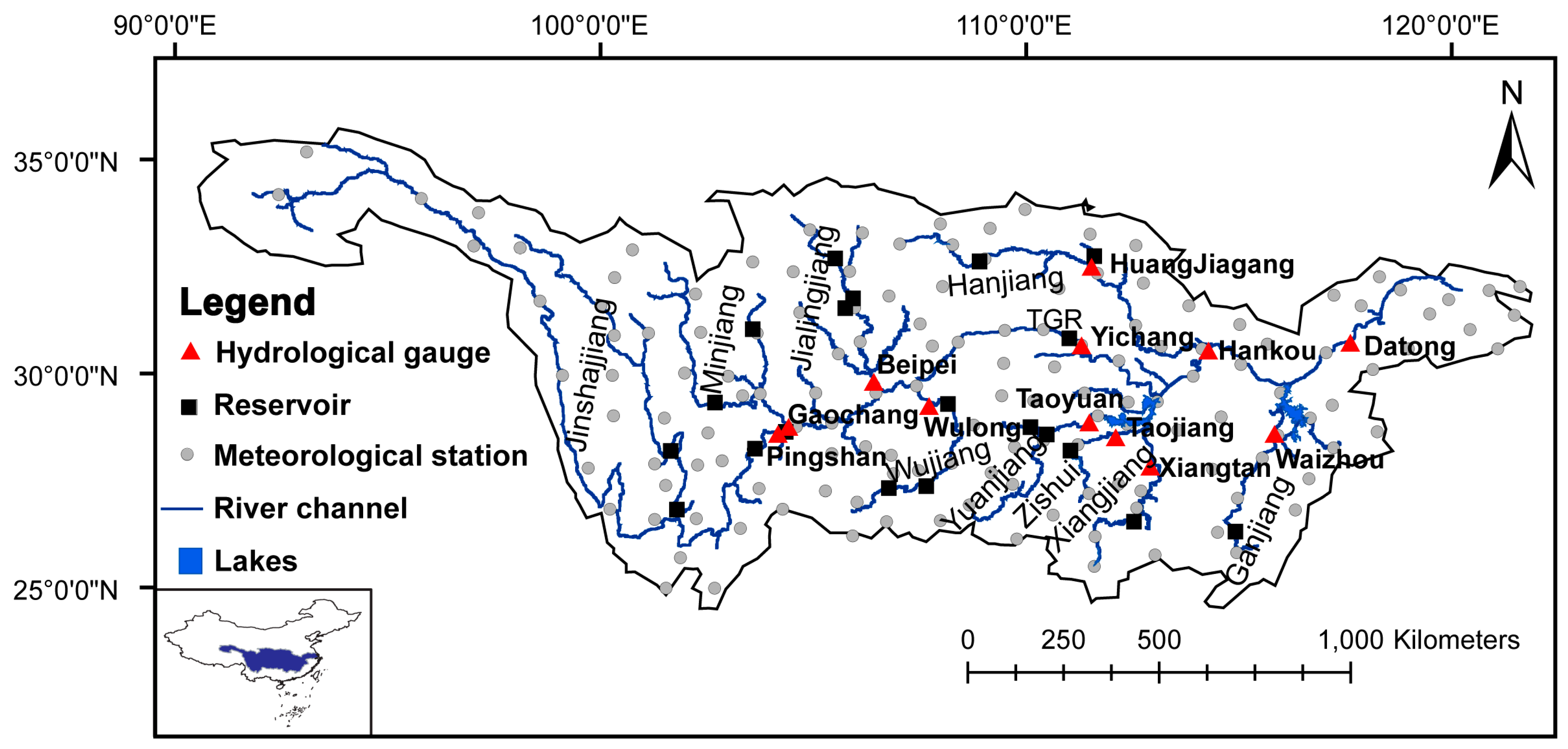
The Yangtze River (Figure 1) originates from the Tanggula Mountain on the Eastern Qinghai-Tibetan Plateau. It flows eastward into the East China Sea and has a length of 6380 km. The Yangtze River Basin has a drainage area of 1.8 million km2, which accounts for 18.8% of the entire area of China. The mean annual precipitation in the Yangtze River Basin is approximately 1070 mm. However, the spatial and temporal variability in precipitation is quite large due to the complex terrain of the Yangtze River Basin and the influence of the monsoon climate. The area upstream of the Yichang gauge (Figure 1) is called the upper reach of the Yangtze River, and the area downstream of the Yichang gauge is called the middle and lower reaches of the Yangtze River. The Yangtze River has abundant freshwater fishery production with more than 200 types of fishes, and the river plays an important role in maintaining the biodiversity of China. On the other hand, the Yangtze River Basin also has abundant hydropower resources. In the past 30 years, many large reservoirs have been constructed for hydro-energy production in the Yangtze River Basin. The major reservoirs in the Yangtze River Basin are summarized in Table 1. The Three Gorges Dam is located approximately 38 km upstream of the Yichang gauge. The TGR entered the first stage of operation in 2003, and it began regular operation at full capacity in 2006.
The observed daily river discharge data from 12 hydrological gauges along the main channel and major tributaries (Figure 1 and Table 2) were provided by the Hydrological Data Center of the Ministry of Water Resources in China. These data were selected to estimate changes in the flow regime because the length of observations at the selected gauges is more than 54 years and because there is at least one large reservoir located in the upstream of each gauge. There are four gauges on the main channel, namely, Pingshan, Yichang, Hankou, and Datong. The area upstream of the Pingshan gauge is also called the Jinshajiang River, and the area upstream of the Yichang gauge is the upper Yangtze River (Figure 1). There are three gauges located at the outlets of tributaries entering the upper Yangtze River: Gaochang, Wulong, and Beibei. There are five gauges on tributaries in the middle and lower Yangtze River, namely, Xiangtan, Taoyuan, Taojiang, Huangjiagang and Waizhou (Figure 1 and Table 2). The observed daily precipitation data from 1961 to 2014 were obtained from 143 meteorological stations (Figure 1) from the China Meteorological Administration [39]. The areal averaged precipitation in the drainage basin of each gauge was calculated using the inverse distance method.
The data used to drive the hydrological model include the atmospheric forcing, land use, soil type, digital elevation model (DEM), and normalized difference vegetation index (NDVI) data. The atmospheric forcing data including daily precipitation, temperature, sunshine hour, wind speed, and relative humidity were provided by the China Meteorological Administration [39]. The DEM data (Figure S1 in the Supplemental Material), with a 90-m spatial resolution, were obtained from the Shuttle Radar Topography Mission (SRTM) dataset [40]. The land use data used in this study were obtained from The Resources and Environment Data Center of the Chinese Academy of Sciences and have a 100 m spatial resolution. The land use data were regrouped into nine categories, including water bodies, urban areas, bare land, forest, cropland, grassland, shrub, wetland, and glacier (Figure S1). The soil type data were provided by the Food and Agriculture Organization (FAO) [41]. The GIMMS (Global Inventory Modelling and Mapping Studies) NDVI data were obtained from Tucker et al. [42].
3. Methodology
3.1. Hydrological Metrics
The IHA metrics were proposed by Richter et al. [13] and comprise 33 parameters in five groups which are shown in Table 3. In this study, a natural period is defined as the period from the year in which the observation started to the year after which the major reservoirs located upstream of the gauge began operating. In the natural period, streamflow is not affected by dam activities. The high flow pulse is defined as the period in which the daily streamflow is greater than the 75th percentile flow during the natural period. The low flow pulse is defined as the period in which the daily streamflow is less than the 25th percentile flow during the natural period. The baseflow index is defined as the seven-day minimum flow divided by the annual mean flow. The number of reversals is calculated by dividing the hydrological record into “rising” and “falling” periods, which correspond to periods when the daily flow changes are either positive or negative, respectively. The dates of the annual minimum and maximum flows are calculated using the Julian date.
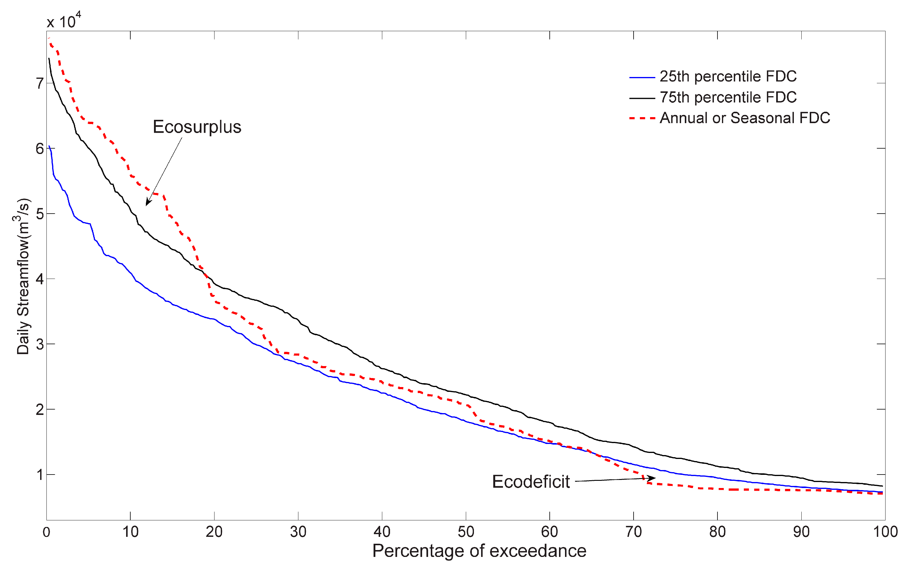
The eco-flow metrics are based on the FDC. The FDC provides a measurement of the time percentage during which a specific flow is equalized or exceeded. To construct an FDC, the observed daily flow data are organized in descending order and the flow Qi is plotted as a function of its corresponding exceedance probability pi. pi is calculated as follows:
where i is the rank corresponding to flow Qi and n is the total number of days. In the present study, both the annual and seasonal FDCs are estimated for each year to analyze the changes in the flow regime. The eco-flow metrics, including ecosurplus and ecodeficit, are calculated using the FDCs. For each gauge, the FDCs in the natural period are used to obtain the 75th percentile FDC and the 25th percentile FDC. Then, the 75th percentile FDC and the 25th percentile FDC are considered the upper and lower bounds of the adaptive range for riverine ecosystems, respectively. If the annual or seasonal FDC of a given year is located above the 75th percentile FDC, the area between the 75th percentile FDC and the annual or seasonal FDC is defined as ecosurplus [23]. Conversely, when the annual or seasonal FDC is below the 25th percentile FDC, the area between the 25th percentile FDC and the annual or seasonal FDC is defined as the ecodeficit (Figure 2). The values of the ecosurplus and ecodeficit are divided by the annual mean or seasonal mean flow to make them dimensionless. Thus, this method makes the eco-flow metrics comparable across different gauges. The ecosurplus represents the amount of streamflow that exceeds the ecosystem requirement and the ecodeficit represents the amount of water lacking in the riverine ecosystem [23].
pi = i/(n + 1)
3.2. Introduction of the Hydrological Model
The geomorphology-based hydrological model (GBHM) [43,44] was used to simulate the natural flow regime of the Yangtze River. The GBHM is a physically based distributed hydrological model for large catchments. A 10-km grid system was used to spatially discretize the whole Yangtze River Basin. A total of 137 sub-basins were identified in the study catchment. Each sub-basin was divided into several flow intervals along the main river channel. A sub-grid parameterization method was used to describe the sub-grid variabilities in topography, which represented a grid characterized by a number of hillslopes with averaged slope lengths and gradients. The hillslopes located within a grid were grouped according to the land use and soil type. Hillslopes represent a fundamental computational unit for hydrological simulation.
The hydrological processes simulated on the hillslopes include snowmelt, canopy interception, evapotranspiration, infiltration, surface runoff, subsurface flow, and the exchange between the groundwater and the river [43,44]. The actual evapotranspiration was calculated from the potential evaporation by considering the seasonal variation in leaf area index (LAI), root distribution and soil moisture availability. The vertical water flow in soil layers was calculated using Richards’ equation and solved by applying an implicit numerical solution scheme. The surface runoff flows through the hillslopes into the stream were calculated via the kinematic wave method. The groundwater aquifer was treated as an individual storage corresponding to each grid. The exchange between the groundwater and the river was considered a steady flow and was calculated according to Darcy’s law [44,45]. The runoff generated from the grid was the lateral inflow into the river at the corresponding flow interval. Flow routing in the river network was solved using the kinematic wave approach. A detailed description of the model can be found in Yang et al. [43,44], Gao [45] and Cong et al. [46].
3.3. Separation of the Impact of Damming and Climate Variation
For each gauge, the data series was divided into two stages: a pre-dam period and a post-dam period. The pre-dam period was from 1961 to the year after which the major reservoirs located upstream of the gauge began operating (Table 2). In the pre-dam period, the streamflow was not affected by dam activities. The post-dam period was from the year in which the major reservoirs started operation to 2014 (Table 2). Therefore, the streamflow in the post-dam period may be affected by dam activities. The model simulation represents the natural flow regime without consideration of reservoir operation. Therefore, the changes in the hydrological metric parameters caused by climate variation between the pre-dam and post-dam periods can be calculated as follows:
where ∆Hclimate is the change in the parameters caused by climate variation. Hsim,post and Hsim,pre are the mean values of the parameters of the hydrological metrics calculated by model simulation in the post-dam period and pre-dam period, respectively.
∆Hclimate = Hsim,post − Hsim,pre
The changes in the parameters between the pre-dam and post-dam periods caused by reservoir operation were calculated as follows:
where ∆Hdam is the change in the parameters caused by reservoir operation and is defined as the difference between the observed change in the parameters (∆Hobs) and the change in the parameters caused by climate variation (∆Hclimate). ∆Hobs was calculated as follows:
where Hobs,post and Hobs,pre are the mean observed values of the parameters of the hydrologic metrics in the post-dam period and pre-dam period, respectively.
∆Hdam = ∆Hobs − ∆Hclimate
∆Hobs = Hobs,post − Hobs,pre
The relative change in the parameters of the hydrological metrics caused by reservoir operation was calculated as follows:
The relative change in the parameters of the hydrological metrics caused by climate variation was calculated as follows:
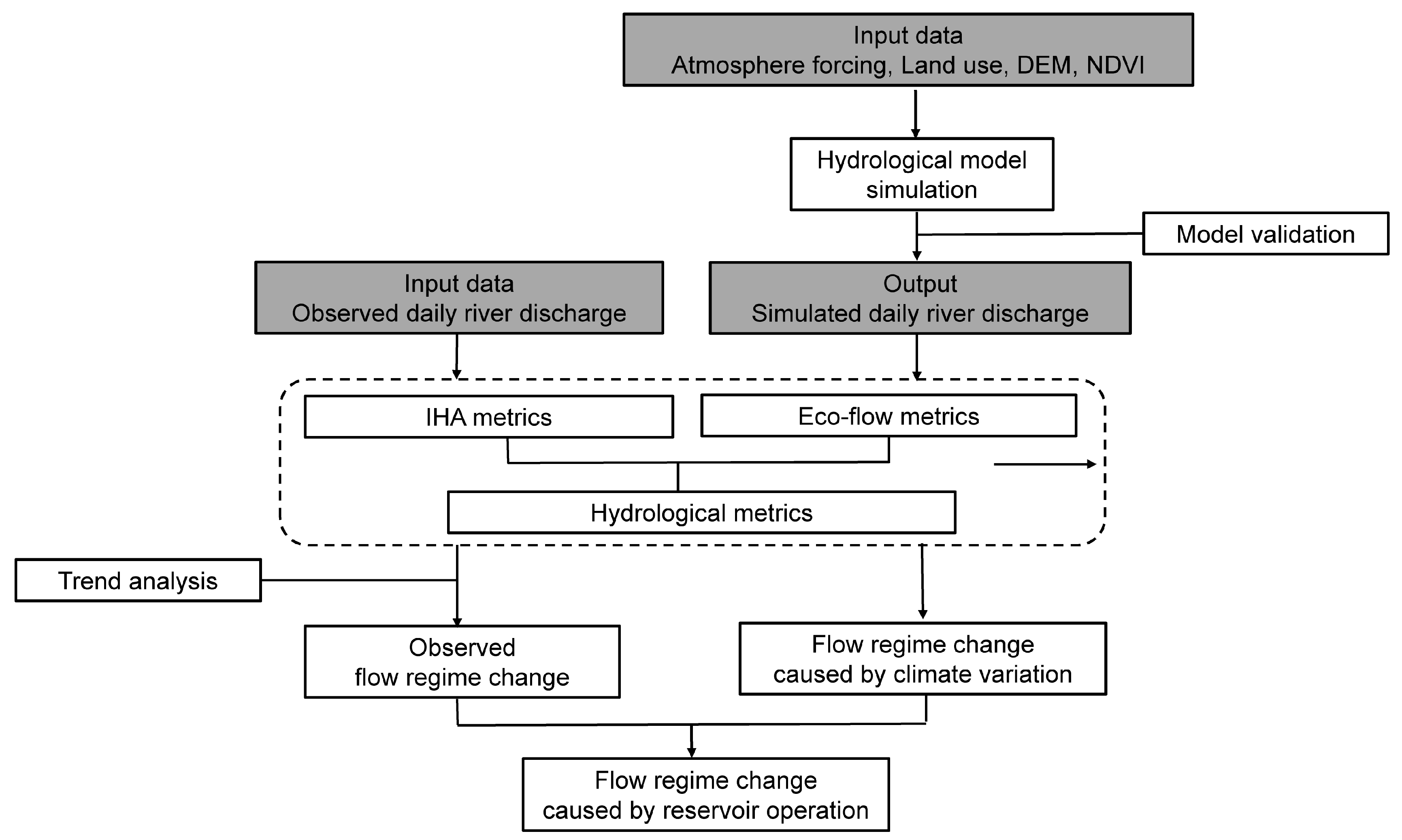
The methodology used in this study is also shown in Figure 3.
4. Results
4.1. Development of a Framework Combining the Eco-Flow Metrics and IHA Metrics
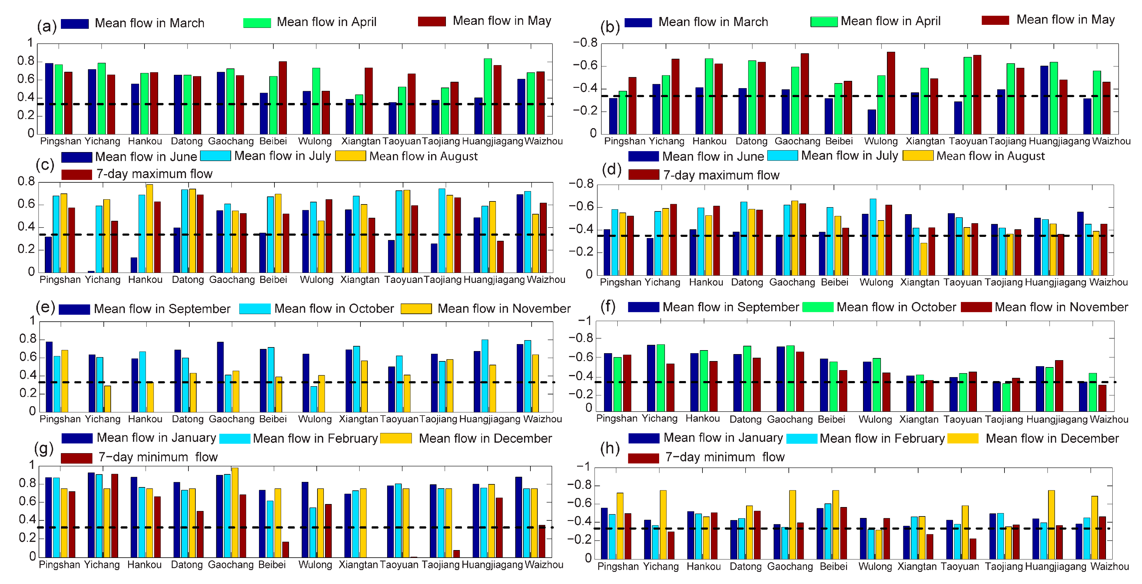
Figure S2 in the Supplement Materials demonstrates that the seven-day minimum flow shows significant correlations with the one-day, three-day, 30-day, and 90-day minimum flows and the baseflow index in group 2 of the IHA metrics. Additionally, the seven-day maximum flow shows significant correlations with the one-day, three-day, 30-day, and 90-day maximum flows. These results imply that the parameters in group 2 are highly inter-correlated and that there is a large degree of statistical redundancy. The seven-day maximum flow and seven-day minimum flow could be considered representative parameters of group 2 of the IHA metrics. The correlation coefficients between the eco-flow metrics and the IHA metrics are shown in Figure 4. This figure shows that the parameters in group 1 (magnitude of monthly streamflow) of the IHA metrics showed significant correlations with seasonal ecosurplus or ecodeficit. The seven-day minimum flow highly correlated with the winter ecodeficit or ecosurplus, and the seven-day maximum flow showed a high correlation with the summer ecodeficit. These results illustrate that the eco-flow metrics can describe changes in the magnitude of the monthly flow and represent changes in the magnitude of the annual extreme flow (parameters in groups 1 and 2 of the IHA metrics). This is consistent with the findings of previous studies [23]. Figure S3 in the Supplemental Materials illustrates that the eco-flow metrics generally show weak correlations with the parameters in groups 3, 4, and 5 of the IHA metrics, although the summer ecosurplus and ecodeficit show high correlations with the rise and fall rates at most gauges. Therefore, in this study, the eco-flow metrics were used to replace the parameters of the first and second groups of the IHA metrics. The metrics used in this study are summarized into two groups (Table 4). The metrics in the first group are the eco-flow metrics, including the annual and seasonal ecodeficit and ecosurplus; these metrics describe changes in the magnitude of the streamflow. The metrics in the second group are the same as the parameters of the third, fourth and fifth groups of the IHA metrics, and these metrics describe the frequency and duration of high and low flow pulses, the rate and frequency of streamflow changes and the timing of the annual extreme flow. This framework includes 19 parameters, which is less than the number of IHA metrics (i.e., 33 parameters). The definitions of the parameters of the second group (Table 4) are the same as those for the IHA metrics. The parameter number of zero flow days is not used in this study, because there are no zero flow days at any gauges in this study. The significance of the trends for all the parameters was examined using the Mann-Kendall non-parametric test [47]. The changes in the hydrological metrics between gauges with different locations were investigated to analyze the spatial changes in the flow regime.
4.2. Changes in Hydrological Metrics
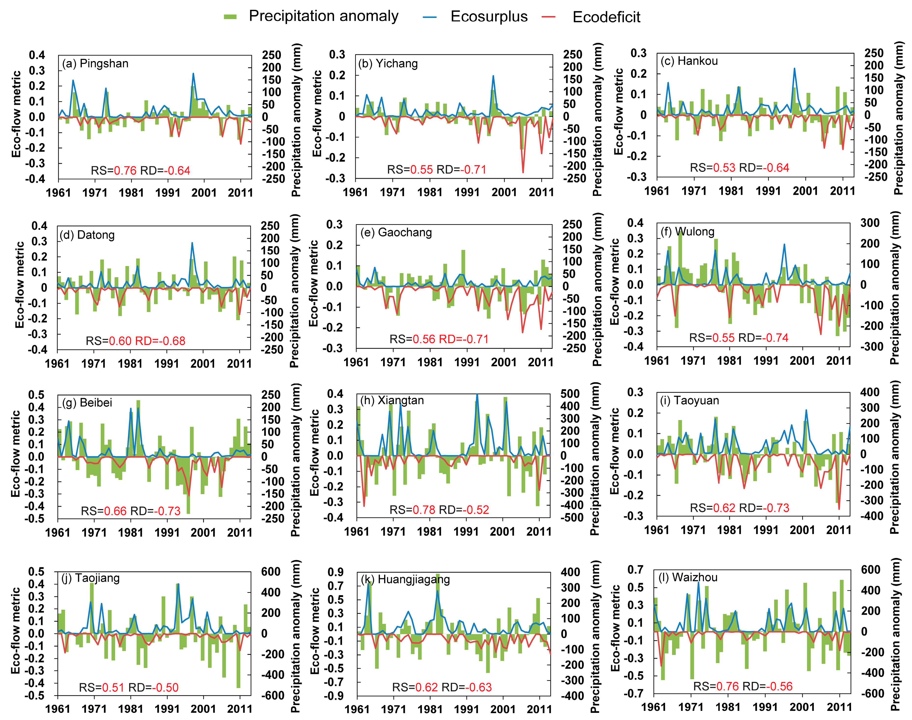
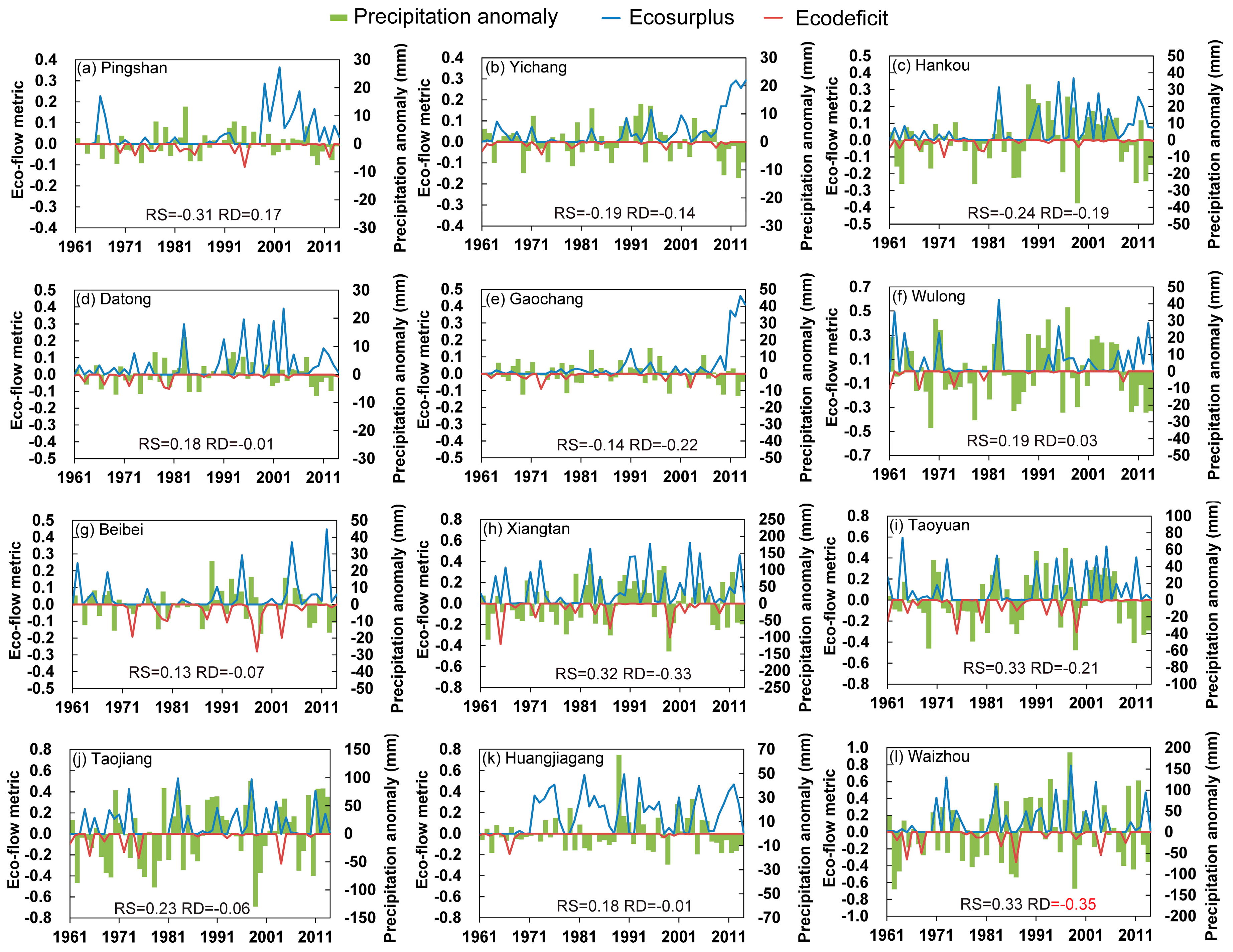
For most meteorological stations, precipitation observations have been available since 1961. Therefore, for each gauge, changes in the metrics during the period of 1961–2014 were examined together with the spatially averaged precipitation in the basin upstream of the gauge. Table 5 shows the linear trends of the parameters of the hydrologic metrics and the results of significance tests for the trends. Figure 5 shows the changes in the annual eco-flow metrics in the period from 2001 to 2014. The magnitude of eco-flow metrics at gauges located on the tributaries was commonly larger than that of the gauges located on the main channel. The magnitude of the eco-flow metrics at the Yichang gauge was similar to those at the Hankou and Datong gauges, even after the TGR started operation in 2003, indicating that the TGR did not have a significant effect on annual streamflow in the main channel. Generally, the eco-flow metrics showed significant correlations with precipitation (evidenced by the correlation coefficients shown in Figure 5), indicating that changes in the annual ecosurplus and ecodeficit were consistent with the changes in annual precipitation. The annual ecosurplus showed decadal variations at the Pingshan, Yichang, Hankou, and Datong gauges along the main channel. The annual ecodeficit clearly increased after the year 2001 at the Yichang and Hankou gauges. The annual ecodeficit also showed significant increasing trends at the gauges located in the tributaries of the upper Yangtze River, particularly the Gaochang and Wulong gauges (Table 5). These results indicated that the annual streamflow decreased significantly in the upper Yangtze River Basin. However, the annual ecodeficit showed no significant changes at the gauges located on the tributaries in the middle and lower Yangtze River Basin except for the Taoyuan gauge and Huangjiagang gauge, which showed a significant increasing trend (Table 5). The annual ecosurplus showed a non-significant decreasing trend at the Xiangtan, Taoyuan, Taojiang, and Huangjiagang gauges, and this trend was generally consistent with changes in precipitation, as illustrated by the correlation coefficient shown in Figure 5.
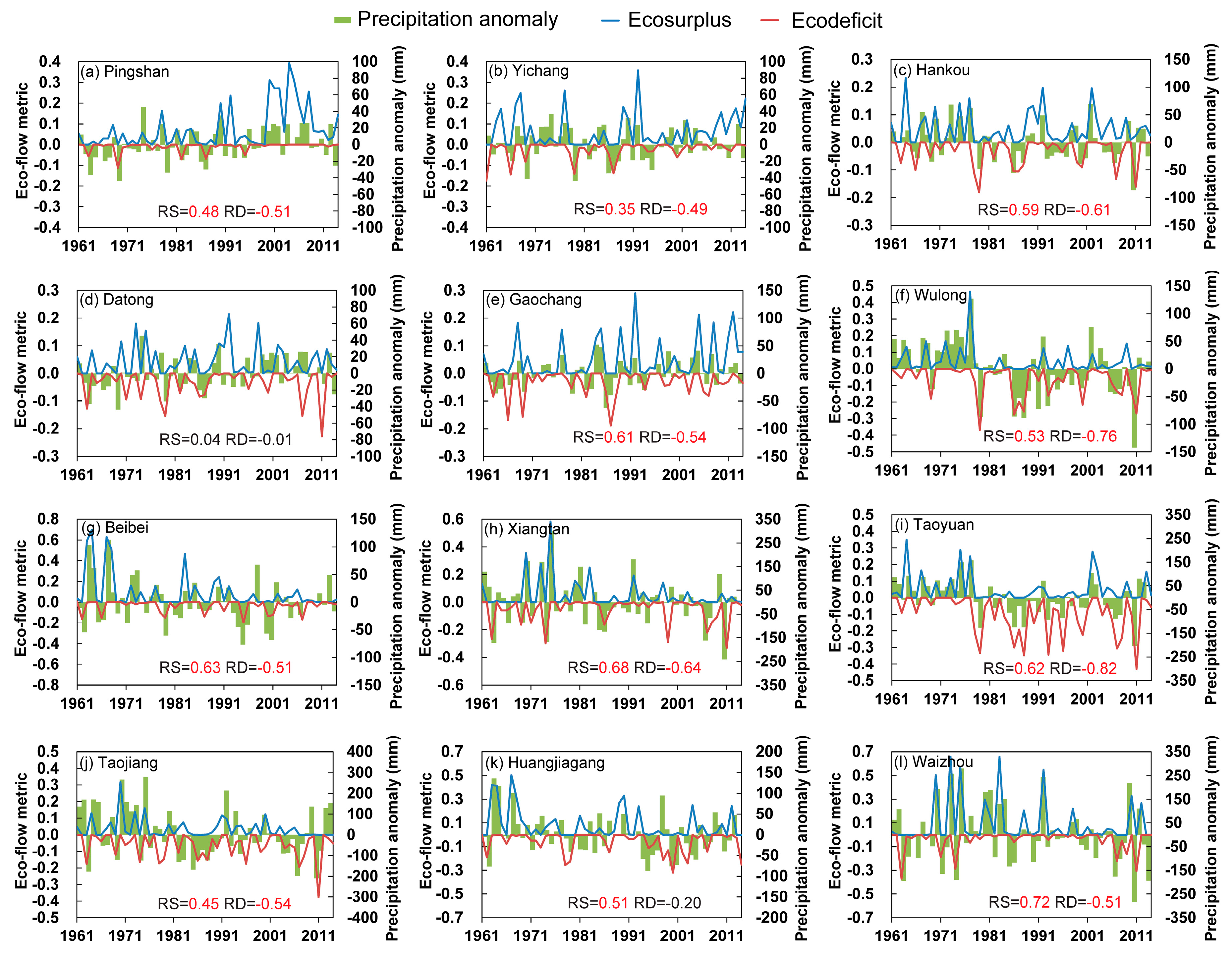
Figure 6 illustrates changes in the ecosurplus and ecodeficit in spring at all gauges. Similar to the annual eco-flow metrics, the magnitudes of ecosurplus and ecodeficit in spring at gauges located on tributaries were generally larger than those on the main channel. For the Pingshan gauge, the spring ecosurplus increased significantly after 1999. This increase was related to the water release of the Ertan Reservoir. No significant changes in the spring ecosurplus and ecodeficit were found at the Yichang gauge before 2003, which was consistent with the changes in precipitation. However, the spring ecosurplus continued to increase after 2003, which is when the TGR started operation. For the Hankou and Datong gauges, the spring ecosurplus and ecodeficit showed no significant changes (Table 5). These results indicate that the TGR had a limited effect on streamflow in the middle and lower reaches of the Yangtze River in spring. For the gauges located on the tributaries of the Yangtze River, the spring ecosurplus and ecodeficit showed significant correlation with precipitation (Figure 6), indicating that changes in the spring ecosurplus and ecodeficit were generally consistent with changes in precipitation. The spring ecosurplus has clearly decreased and the ecodeficit has clearly increased since 1981 at the Wulong gauge and Taoyuan gauge (Table 5), because of a decrease in precipitation. These results suggest that a decline in precipitation led to a significant decreasing trend in the streamflow in spring in the Wujiang River Basin and Yuanjiang River Basin.
Figure 7 shows the changes in the ecosurplus and ecodeficit in summer for all gauges. Generally, the ecosurplus and ecodeficit showed no significant changes at gauges located along the main channel (Table 5). For the gauges located on tributaries of the upper Yangtze River, a significant increase in the summer ecodeficit was observed starting in 2004 at the Gaochang gauge, which was not consistent with the changes in precipitation. This result may be related to the operation of the Zipingpu Reservoir which started in 2004, and the operation of the Pubugou Reservoir, which started in 2008. The summer ecodeficit also clearly increased at the Wulong gauge starting in 2004 because of the associated decrease in precipitation. For the gauges in the middle and lower reaches of the Yangtze River, in general, the summer ecosurplus and ecodeficit showed no evident changes (Table 5).
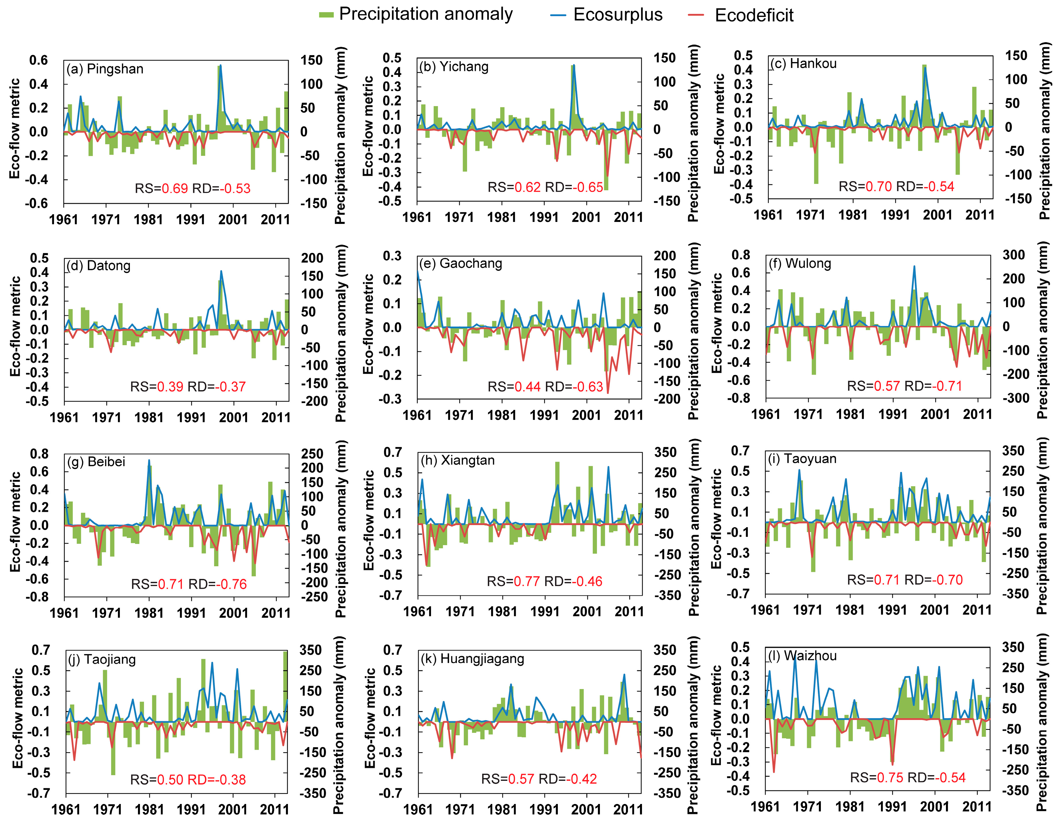
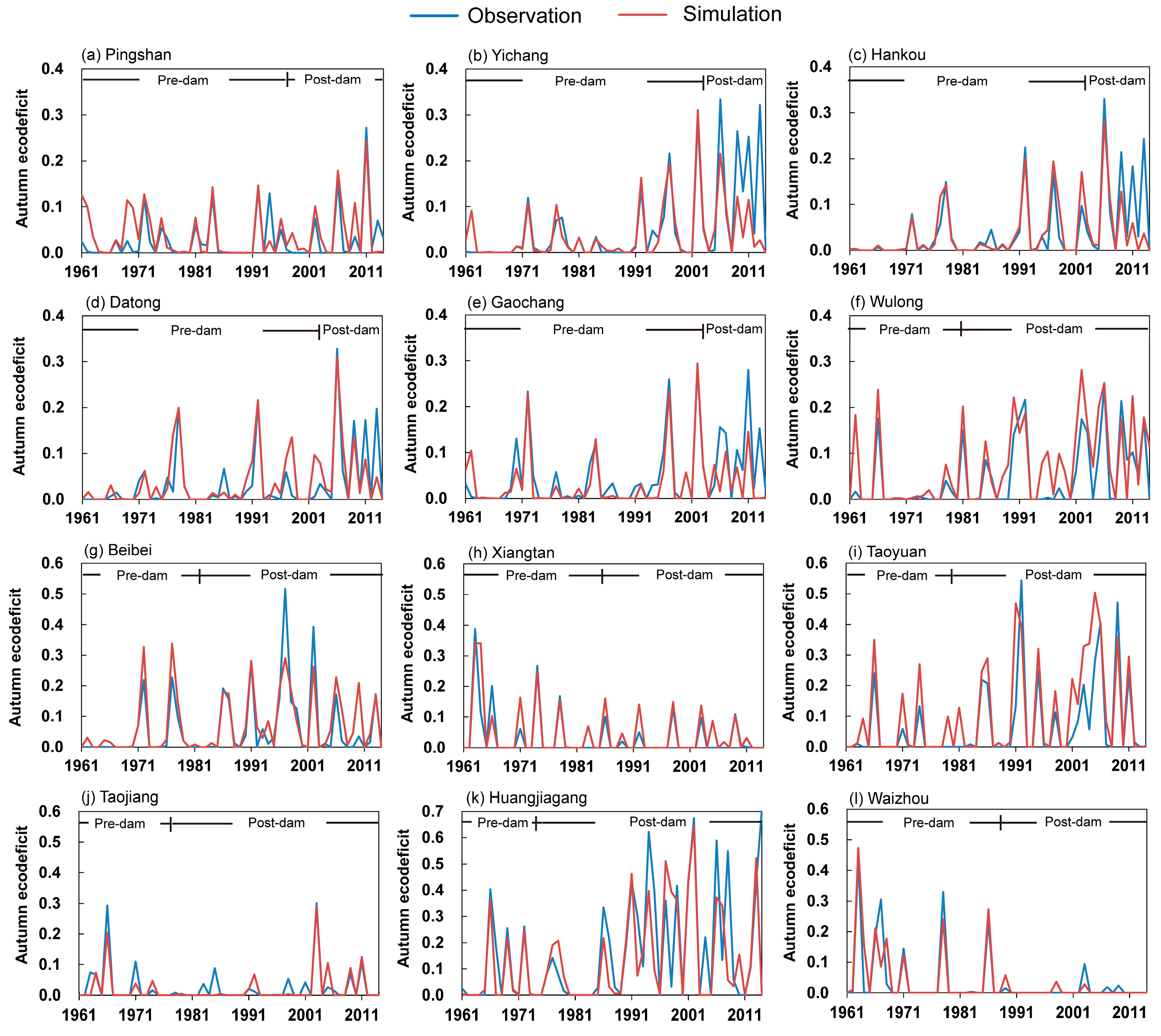
The eco-flow metrics showed larger changes in autumn and winter than in summer and spring. Figure 8 illustrates the changes in the ecosurplus and ecodeficit in autumn. The autumn ecosurplus decreased at all gauges along the main channel, particularly after 2001. The autumn ecodeficit clearly increased at the Yichang, Hankou and Datong gauges (Table 5), particularly after 2003, which is when the TGR started operation. This result illustrates that the autumn streamflow decreased significantly in the main channel of the Yangtze River. Significant increases in the ecodeficit were also found at all gauges located on the tributaries of the upper Yangtze River (Table 5). This result implies that the autumn streamflow significantly decreased in the tributaries of the upper Yangtze River Basin. As shown in Figure 8, the streamflow at the Gaochang and Wulong gauges located on tributaries of the upper Yangtze River showed stronger decreasing trends than the trend of the precipitation anomaly (Figure 8e,f). This result indicates that the decreased precipitation was not the only factor contributing to the decrease in streamflow; dam construction may be another reason. Generally, the autumn ecosurplus and ecodeficit showed no significant changes at most gauges located on the tributaries of the middle and lower Yangtze River Basin (Table 5). However, the Huangjiagang gauge and Taoyuan gauge have shown a significant increase in the autumn ecodeficit since 1981.
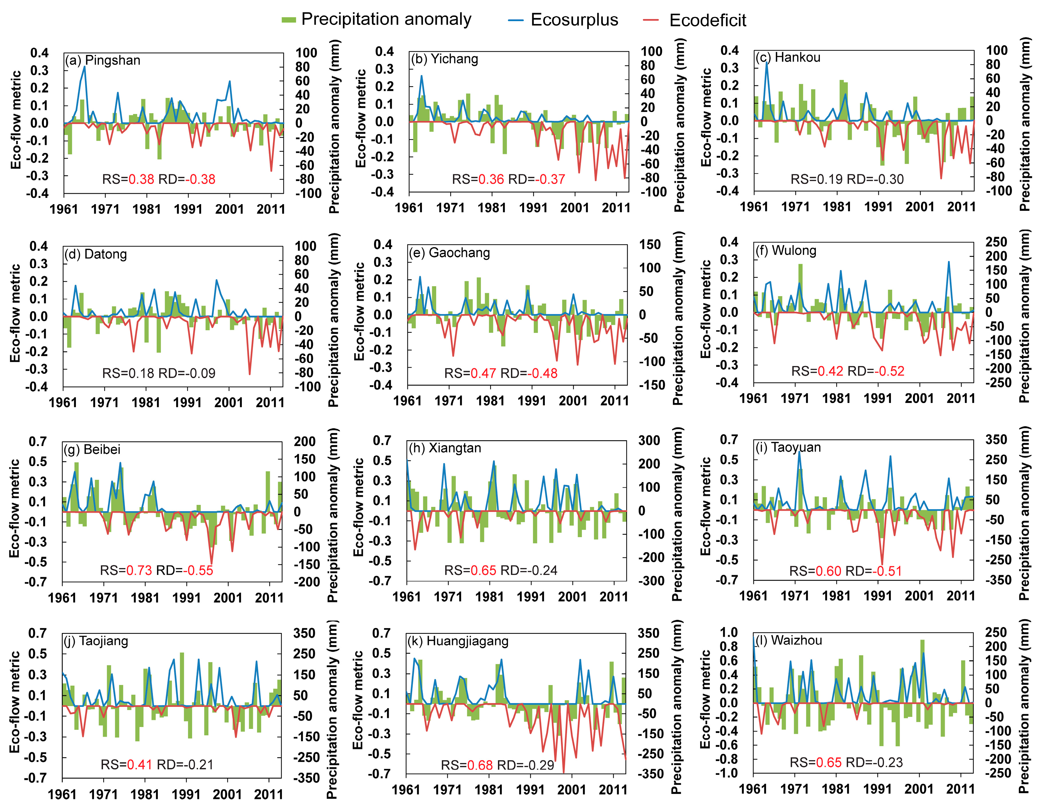
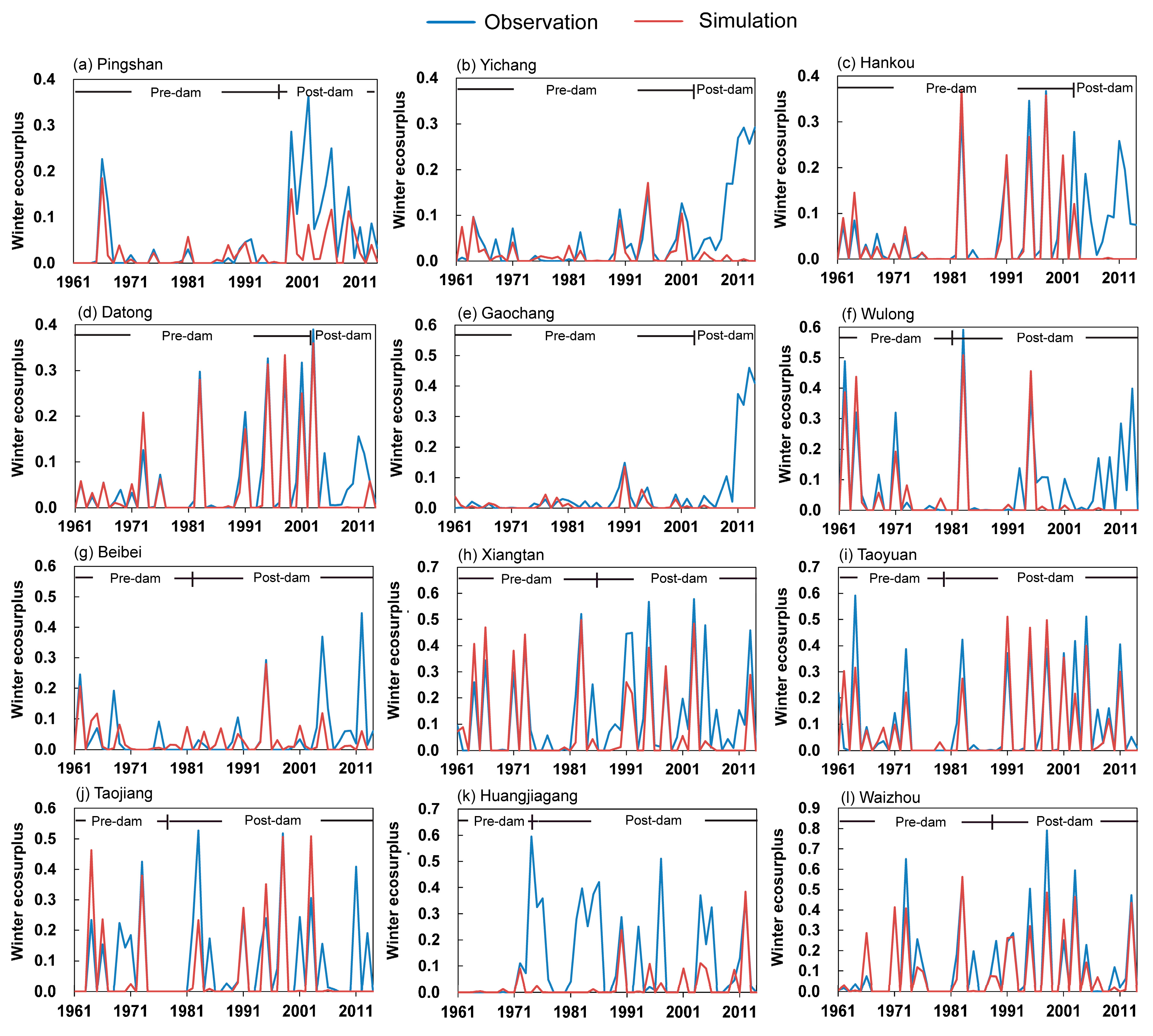
Figure 9 shows the changes in the ecosurplus and ecodeficit in winter. The winter ecosurplus increased at all gauges along the main channel. Moreover, the winter ecosurplus has increased significantly at the Pingshan gauge since 1999, which is when the Ertan Reservoir began operating. The winter ecosurplus also increased abruptly at the Yichang and Hankou gauges after the TGR began operating at full capacity in 2006, despite the negative precipitation anomaly observed since 2006 (Figure 9b,c). The winter ecosurplus significantly increased at the Gaochang, Wulong, and Beibei gauges, which are located on the tributaries of the upper Yangtze River Basin (Table 5). The increase in the ecosurplus at the Gaochang gauge was not consistent with changes in precipitation (Figure 9e), and a weak correlation between the winter ecosurplus and precipitation was observed (r = −0.14). This finding implies that the increase in winter streamflow in the Minjiang River may be related to reservoir operation. The winter ecosurplus and ecodeficit showed no significant changes at most gauges in the middle and lower Yangtze River Basin, with the exception of the Huangjiagang gauge, which showed a significant increasing trend for ecosurplus (Table 5).
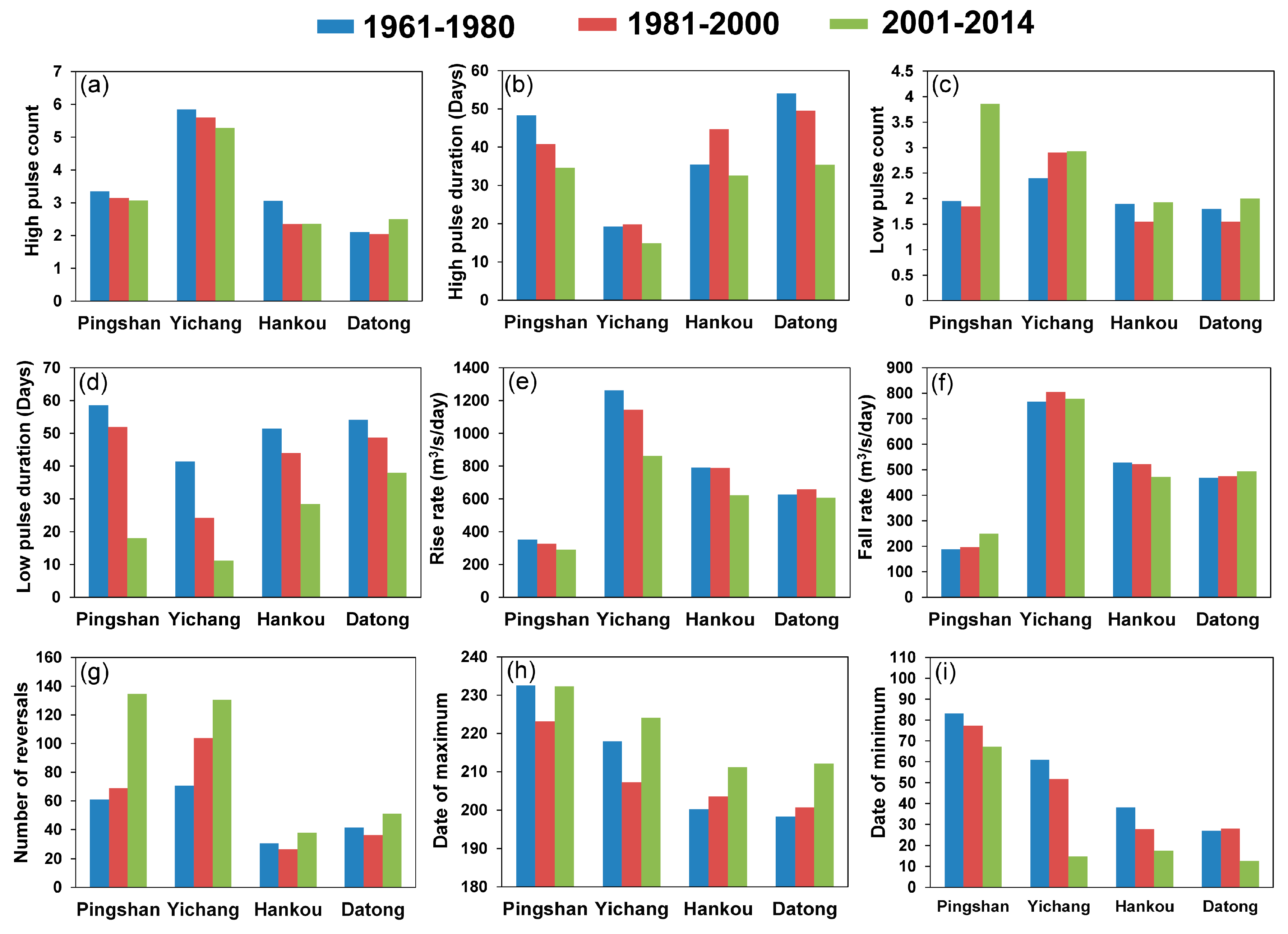
Table 5 and Figure 10 present the changes in the parameters of the group 2 hydrological metrics at the gauges located on the main channel. The spatial changes in the parameters can be observed in Figure 9. Number of reversals and the rise and fall rate of flow were larger at the Yichang gauge than at the Hankou and Datong gauges. This pattern may be because the topography in the upper Yangtze River Basin is much steeper than that in the middle and lower Yangtze River. Generally, the high and low pulse counts showed no significant changes during the period of 1961–2014, except at the Pingshan gauge, for which the low pulse count showed a significant increase (Figure 10a,c). The low flow pulse durations decreased significantly at the gauges located along the main channel (Table 5). The rise rate of flow was significantly reduced at the Yichang and Hankou gauges, but it showed no significant changes at the other gauges. The fall rate of flow showed no significant changes for all gauges along the main channel. A significant increase in the number of reversals was found at the Pingshan and Yichang gauges (Table 5). A slight delay in the date of the annual maximum flow and a significant advance in the date of the annual minimum flow were found at the Yichang, Hankou and Datong gauges (Figure 10 and Table 5).
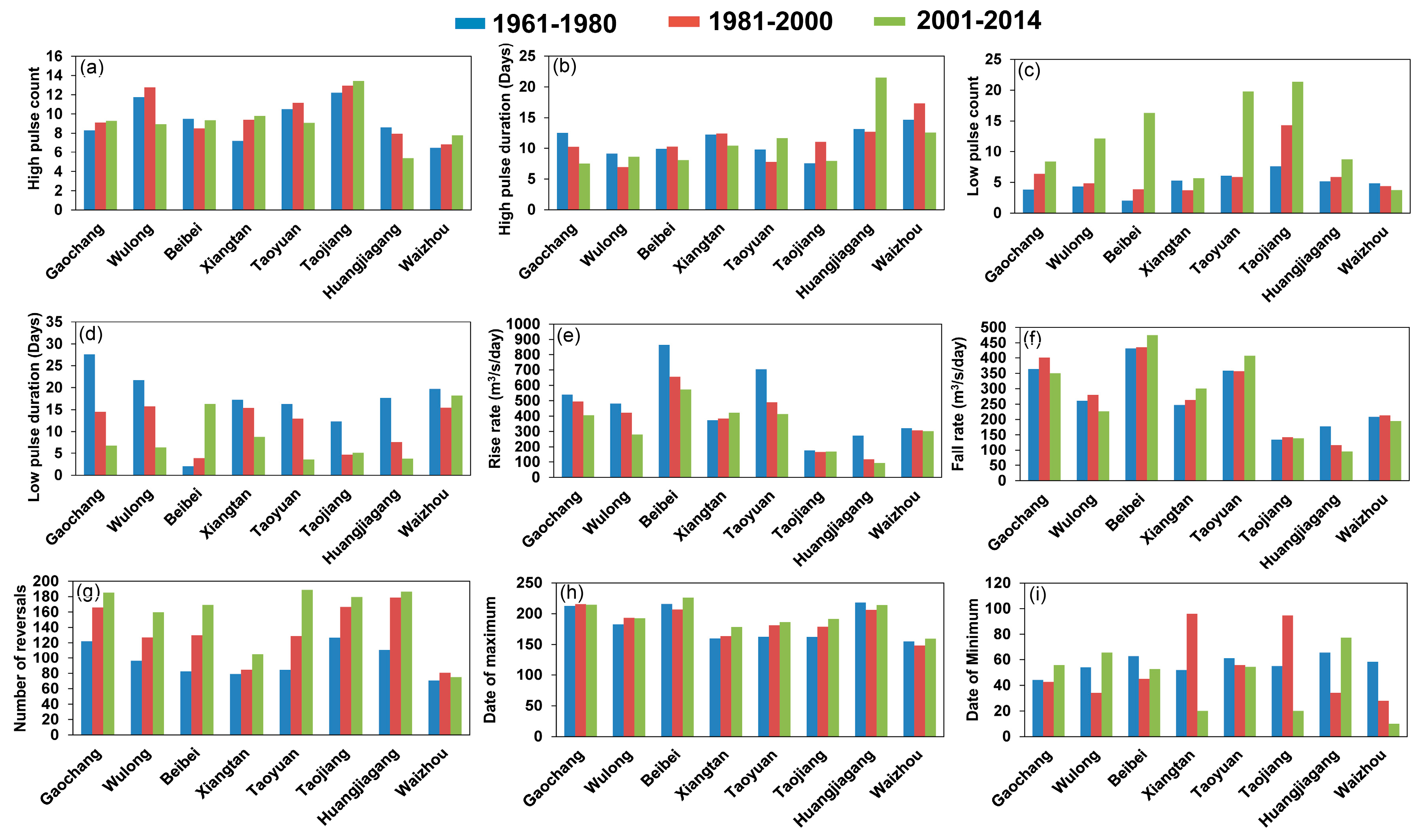
Table 5 and Figure 11 show the changes in the parameters of the group 2 hydrological metrics at gauges located on the tributaries. A comparison of Figure 10 and Figure 11 shows that there were generally more high and low pulse counts but shorter high and low pulse durations at the gauges located on the tributaries than at the gauges located on the main channel. This difference may be related to the differences in drainage area between gauges located on the main channel and those located on the tributaries. Figure 11 and Table 5 reveal that the high pulse count showed no significant changes during the period from 1961 to 2014, except at the Wulong gauge and Huangjiagang gauge, at which the counts have decreased significantly since 2001. The high pulse duration showed no significant changes at most gauges. Only the Gaochang gauge showed a significant decreasing trend, and the Huangjiagang gauge showed a significant increasing trend. The low pulse count commonly showed a significant increasing trend, except at the Waizhou gauge and Xiangtan gauge. In contrast, the low pulse duration commonly showed a significant decreasing trend (Table 5). However, the low pulse duration showed no significant changes at the Waizhou gauge, and a significant increasing trend was observed at the Beibei gauge. The rise rate of flow showed a significant decreasing trend at most gauges, except the Xiangtan gauge, Taojiang gauge, and Waizhou gauge, which showed no significant changes. The fall rate of flow showed no significant changes, except at the Huangjiagang gauge. The number of reversals showed a significant increasing trend for all gauges except the Waizhou gauge, which did not show significant changes. The date of the annual maximum flow showed no significant changes for all gauges. However, the date of the annual minimum flow significantly decreased at the Beibei, Xiangtan, Taojiang, and Waizhou gauges.
4.3. Validation of the Hydrological Model
The period of 1961–1965 was used to calibrate the GBHM model and the following period of 1966–1970 was used for model validation. The major calibrated parameters included the surface water retention capacity and the roughness of the river channel. The model performance in simulation of the daily river discharge is shown in Figure S4 and Table S2 in the Supplemental Material. The model simulation agrees well with the observed discharge in both the calibration and validation periods (Figure S4). The Nash-Sutcliffe efficiency (NSE) coefficient was larger than 0.7 for all gauges, except the Beibei and Huangjiagang gauge which had NSE values of 0.68 and 0.69 in the validation period, respectively (Table S2). The relative error (RE) was within 5% for all gauges, except for the Taojiang gauge which had an RE value of −7.3% in the validation period.
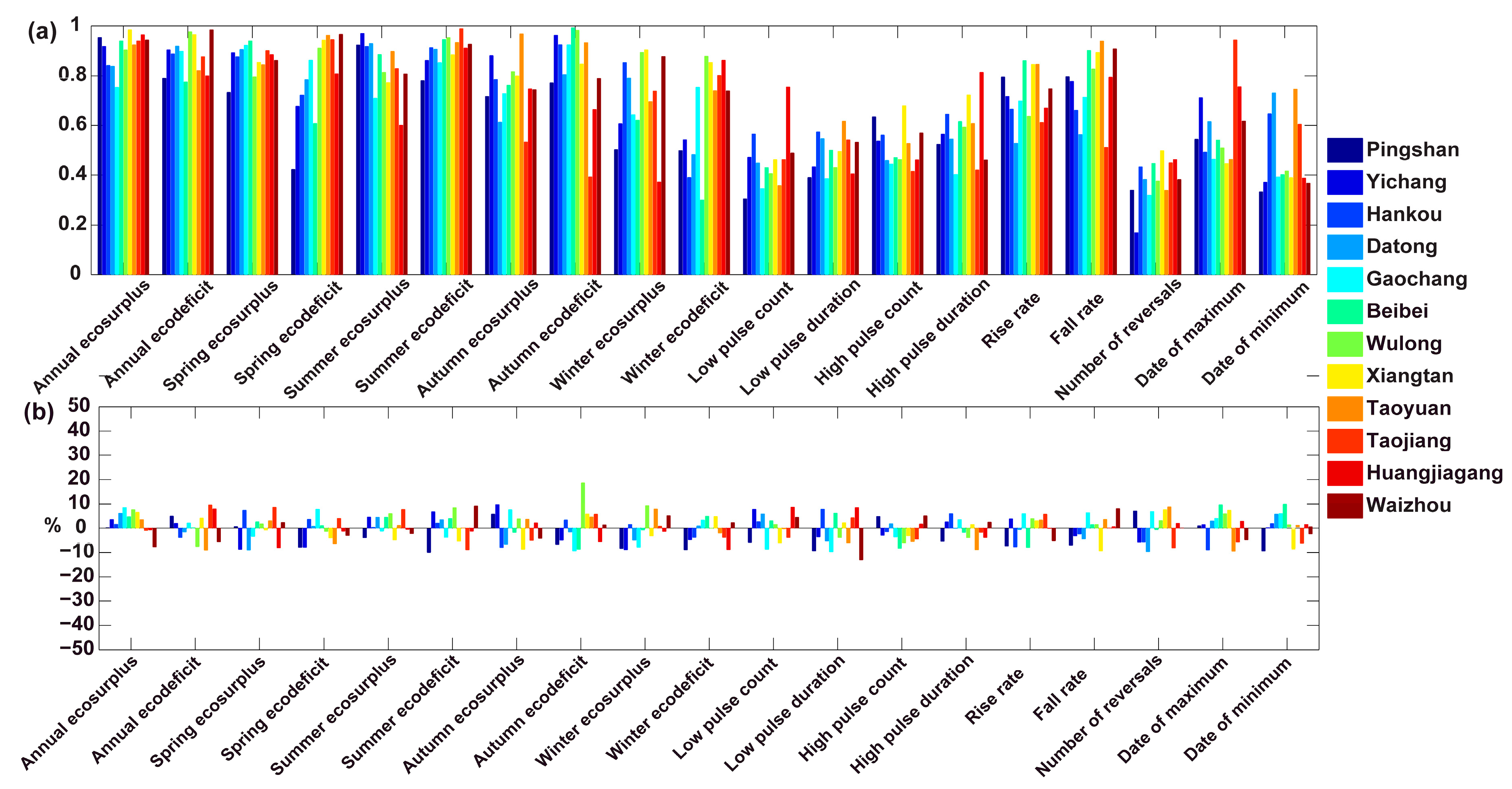
The model skill in simulating the hydrologic metrics was also validated. Figure 12 shows the correlation coefficient between the parameters of hydrologic metrics calculated by observation and model simulation. The model-simulated parameters showed high correlation with the observations and the REs were within 10% at most gauges. Therefore, the model effectively captured the changes in the hydrologic metrics at all the selected gauges.
4.4. Impacts of Dams on Flow Regime
Based on the results described in Section 4.2, the winter ecosurplus, autumn ecodeficit, low pulse count, low pulse duration, number of reversals, rise rate, and date of annual minimum flow showed larger changes than the other parameters. Therefore, these parameters were selected to further investigate the impacts of dams on the flow regime. The changes in parameters based on the observed and model-simulated daily river discharge values were analyzed.
Figure 13 illustrates the changes in the autumn ecodeficit between the pre-dam and post-dam periods. As shown in the figure, the model-simulated autumn ecodeficit was close to the observations in the pre-dam period at the Yichang, Hankou, and Datong gauges. However, the model-simulated ecodeficit was lower than the observations in the post-dam period. These results illustrate that water storage in the TGR significantly reduced the autumn streamflow in the main channel of the middle and lower reaches of the Yangtze River. Similar changes were found at the Gaochang gauge located on a tributary of the upper Yangtze River. These results indicate that water storage of the reservoirs was one of the major causes of the decrease in the autumn streamflow in the Minjiang River in the upper Yangtze River Basin. For the gauges located on the tributaries of the middle and lower Yangtze River, the model-simulated parameters were close to the observations. Therefore, the changes in the autumn ecodeficit in the tributaries of the middle and lower Yangtze River were mainly caused by climate variation.
Figure 14 illustrates the changes in the winter ecosurplus between the pre-dam and post-dam periods. In the pre-dam period, the model-simulated winter ecosurplus was close to the observations at the Pingshan, Yichang, Hankou, and Datong gauges. However, the observed winter ecosurplus was significantly larger than the model-simulated ecosurplus in the post-dam period. Therefore, the increase in the winter ecosurplus in the main channel was mainly caused by the release of water from the reservoirs. The Gaochang gauge and Wulong gauge located on the tributaries in the upper Yangtze River, also showed notable differences between the model simulation and the observations in the post-dam period. The model-simulated winter ecosurplus was close to the observations in the post-dam period at the Taoyuan gauge and Waizhou gauge located on tributaries of the middle and lower Yangtze River, which implies that reservoir operation did not have a significant impact on the winter streamflow in the Yuanjiang and Ganjiang tributaries. Compared with the pre-dam period, the observed winter ecosurplus at the Huangjiagang gauge in the post-dam period showed a much larger increase than the model-simulated ecosurplus, indicating that reservoir operation was the major factor contributing to the increase in the winter streamflow in the Hanjiang River. For the Xiangtan gauge and Taojiang gauge, the observed winter ecosurplus was significantly larger than the model simulation during some of the −s in the post-dam period. This finding implies that the impact of reservoir operation on the winter streamflow cannot be ignored in the Xiangjiang River and the Zishui River.
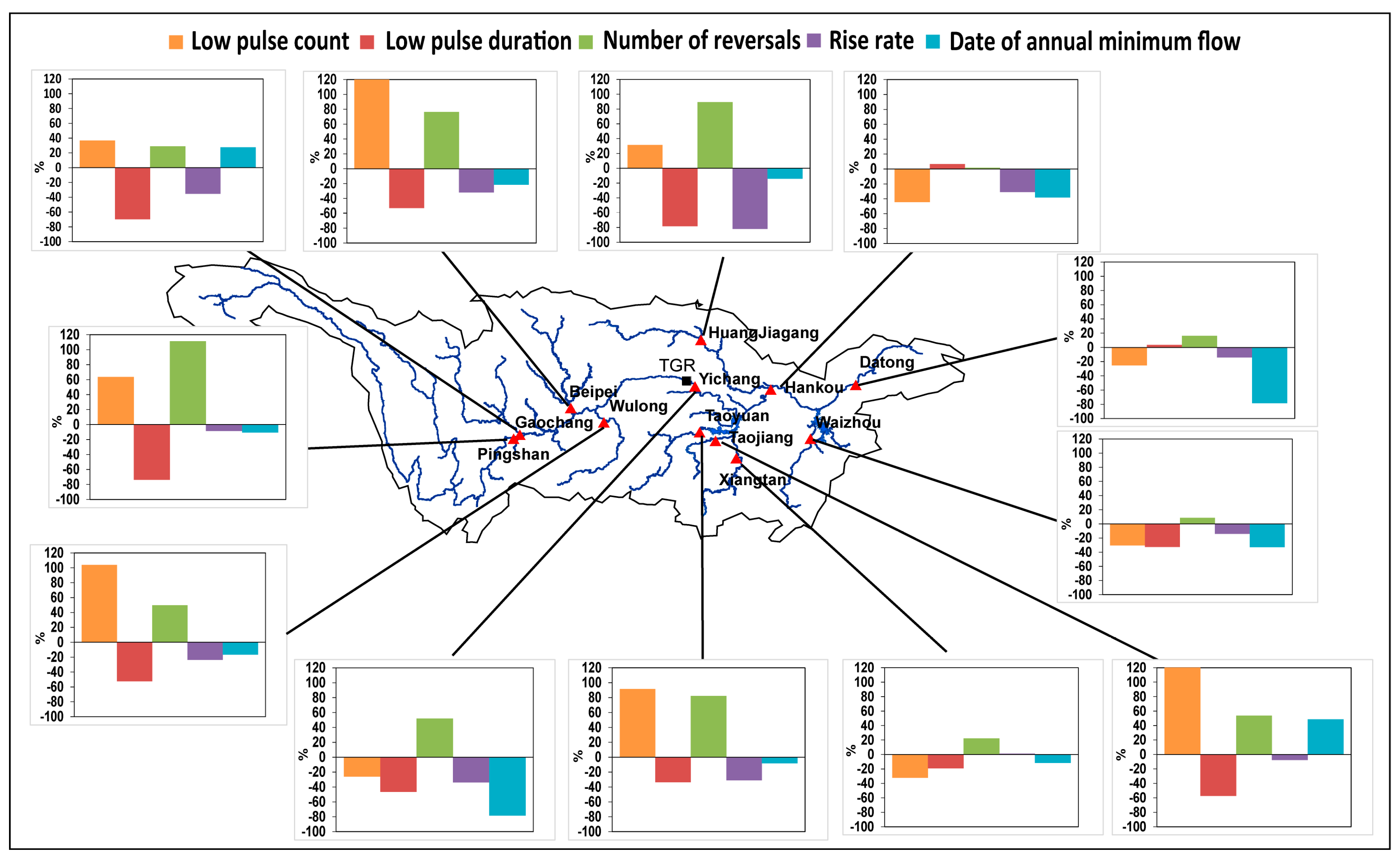
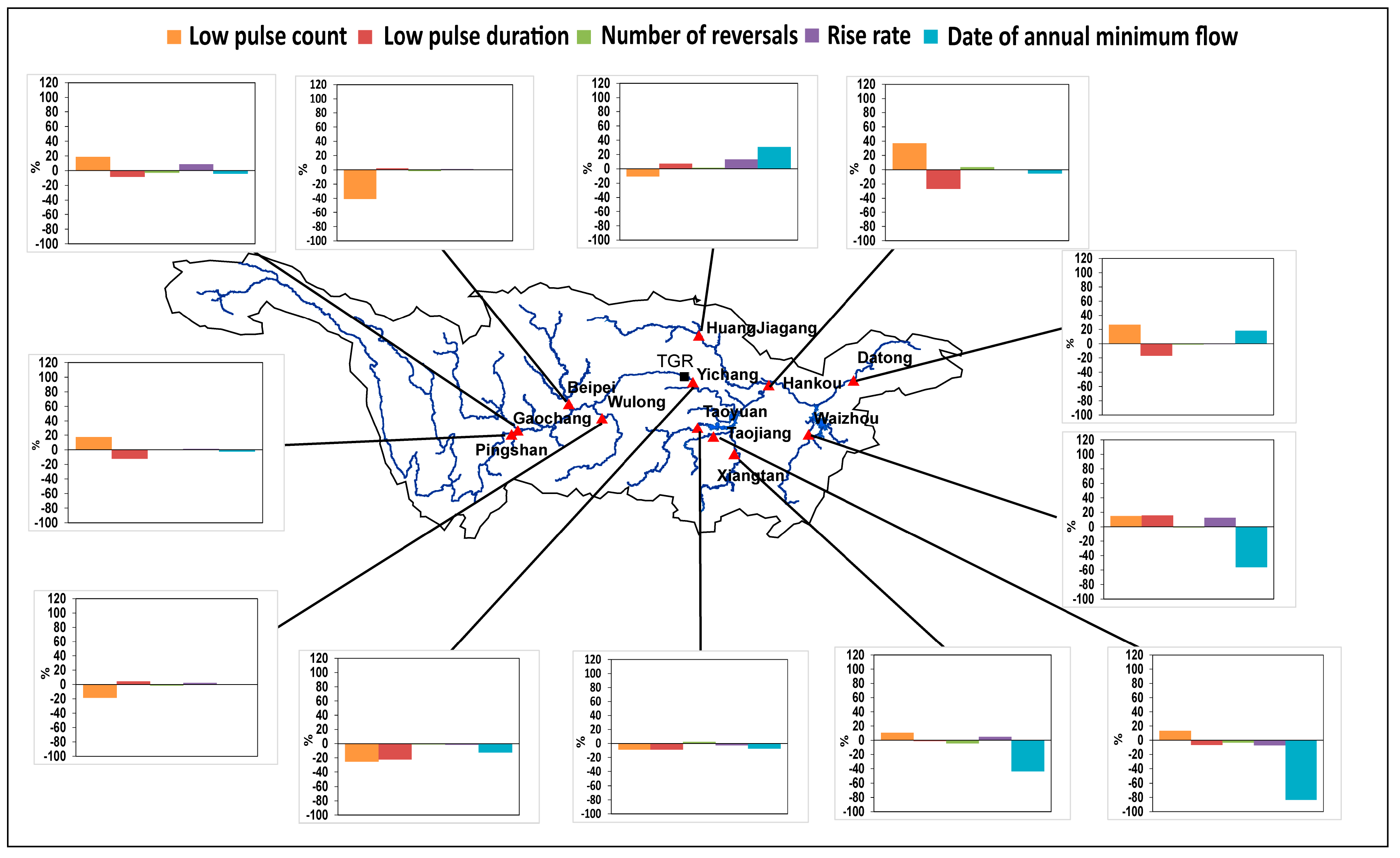
The relative changes in low pulse count, low pulse duration, number of reversals, rise rate, and date of annual minimum flow caused by reservoir operation (calculated by Equation (5)) and climate variation (calculated by Equation (6)) are shown in Figure 15 and Figure 16, respectively. As shown in Figure 15, compared with the pre-dam period, the increase in the low pulse count caused by reservoir operation in the post-dam period at the Pingshan gauge was approximately 60%, and the reduction in the low pulse duration caused by reservoir operation was more than 60%. These changes were much larger than those caused by climate variation, as shown in Figure 16. At the Yichang gauge, the decrease in the low pulse count caused by reservoir operation was more than 20% and was close to the relative change caused by climate variation (Figure 16). Reservoir operation led to an approximately 40% decrease in the low pulse duration at the Yichang gauge in the post-dam period, which was larger than the changes caused by climate variation. This result was related to the water released from the TGR in winter and spring. The relative changes in the number of reversals caused by reservoir operation were larger than 40% at the Pingshan and Yichang gauges, and the changes caused by climate variation were close to zero. For the Hankou gauge, the relative changes in the low pulse count caused by reservoir operation and climate variation were comparable in magnitude but different in direction. Thus, no significant change in the observed low pulse count was found for the Hankou gauge, as shown in Figure 10. The changes in the low pulse duration and the number of reversals caused by reservoir operation were less than 10% at the Hankou gauge. However, a significant reduction in the low pulse duration caused by climate variation was detected (Figure 16), indicating that climate variation was one of the major reasons for the reduction of low pulse duration in the middle reach. Similar results were found at the Datong gauge. These results indicate that the TGR exerted a significant impact by increasing the frequency of low flow pulses but showed no significant effect on the low flow duration and the frequency of flow changes in the middle and lower reaches of the Yangtze River. For the gauges located on tributaries, significant increases in the low pulse count and the number of reversals but significant decreases in the low pulse duration caused by reservoir operation were found at most gauges, with relative changes of greater than 20%. These changes were much larger than those caused by climate variation as shown in Figure 16, implying that reservoir operation was the primary factor contributing to the increase in the frequency of low flow, the decrease in the duration of low flow and the increase in the frequency of flow changes in most tributaries.
The changes in the rise rate of flow and the date of the annual minimum flow caused by reservoir operation and climate variation are also shown in Figure 15 and Figure 16. It can be observed from the figure that changes in the rise rate of flow between the post-dam and pre-dam periods caused by reservoir operation were larger than 20% at the Yichang and Hankou gauges. The changes in the rise rate of flow caused by climate variation were close to zero. These results imply that the operation of the TGR was the major cause for the reduction in the rise rate of flow in the middle reaches of the Yangtze River. Figure 15 illustrates that a significant decrease in the rise rate of flow caused by reservoir operation was also found at gauges located on the tributaries of the upper Yangtze River and at the Taoyuan gauge and the Huangjiagang gauge on tributaries of the middle and lower Yangtze River. These changes were also much larger than the changes caused by climate variation as shown in Figure 16. Reservoir operation also led to a significant decline in the date of the annual minimum flow at the Yichang, Hankou, and Datong gauges in the post-dam period (Figure 15), and climate variation had little effect on the changes in the date of the annual minimum flow (Figure 16). This result illustrates that the operation of the TGR led to an earlier occurrence of the annual minimum flow in the middle and lower reaches. Generally, reservoir operation dominated the changes in the date of the annual minimum flow in the tributaries of the upper Yangtze River, and climate variation showed a larger effect on the date of the annual minimum flow than reservoir operation in tributaries of the middle and lower Yangtze River.
5. Discussion
5.1. Possible Implications of Flow Regime Change for Aquatic Biota
A decrease in the autumn high flows in the main channel reduced the transport of sediment and organic resources and caused a decline in the habitat suitability for some fish species. A decrease in the autumn streamflow also reduced the water level and the areas of the Dongting Lake and the Poyang Lake though river-lake interactions, greatly affecting the ecosystem of the two lakes, including reductions in the habitats of many important fish and bird species.
An increase in the winter flow indicates an increase in the magnitude of low flows, which may create conditions that are unfavorable to native species and beneficial to other species. The timing of extreme flows is an important environmental cue for initiating life cycle transitions. An earlier occurrence of the annual minimum flow may affect the migration and spawning of some fish species.
An increase in the number of flow reversals and the low flow frequency may cause life cycle disruptions and a loss of some species that are sensitive to the frequency of flow variations. The reduction in the rise rate of flow greatly affected the spawning of some fish species, particularly in the middle and lower Yangtze River Basin.
The construction of dams continues on in the Yangtze River, particularly in the upper Yangtze River. For example, the Baihetan Reservoir and the Wudongde Reservoir, which are under construction on the Jinshajiang River, have capacities of 206 × 108 m3 and 74 × 108 m3, respectively. Their construction will cause large changes in the flow regime of the Yangtze River. Future studies are needed to incorporate the consideration of changes in hydrological metrics into the operation rules of multiple reservoirs in the Yangtze River Basin.
5.2. Comparison of the Eco-Flow Metrics with the IHA Metrics
The magnitude of the monthly streamflow showed a significant correlation with ecosurplus or ecodeficit (or both) in the same season (Figure 4). Therefore, the eco-flow metrics could describe major changes in the parameters of group 1 of the IHA metrics with fewer parameters. The magnitudes of extreme flows with different durations showed significant inter-correlations indicating that there is information redundancy in the parameters of group 2 of the IHA metrics. The eco-flow metrics in summer and winter are significantly correlated with the parameters describing the magnitudes of high and low flows, respectively (Figure 4). Therefore, the eco-flow metrics effectively capture the changes in the parameters of group 2 of the IHA metrics. These results show that the eco-flow metrics can describe changes in the magnitude of the monthly streamflow and extreme flow more effectively than the IHA metrics. However, the eco-flow metrics show weak correlation with parameters in the third, fourth and fifth groups of the IHA metrics (Figure S3 in the Supplemental Materials). Only the summer ecosurplus and summer ecodeficit showed significant correlations with the rise rate and fall rate of flow at most gauges, meaning that the eco-flow metrics can capture characteristics of the rate of flow changes but are unable to describe other parameters related to the frequency and duration of extreme flows, the frequency of flow change and the timing of extreme flows. This pattern is probably because the eco-flow metrics are calculated by FDCs. FDCs are related to the probability of different magnitudes of flows and may lose information on the timing and duration of extreme flows.
5.3. Comparison with Recent Similar Studies
Talukdar and Pal [48] analyzed the impact of dams on flow regime changes in the Punarbhaba River Basin of Indo-Bangladesh using some of the parameters in IHA metrics and found that dam construction increased the low flow in the dry season and reduced the high flow in autumn. However, the impact of the dams was not separated quantitatively from the impact of climate in their study. They also found that the mean flow in summer and the annual maximum flow significantly decreased in the post-dam period. This finding is different from the results of the current study. The difference is because reservoirs in the Punarbhaba River Basin are mainly designed to supply water for irrigation, whereas reservoirs in the Yangtze River are mainly for hydropower generation. Pumo et al. [49] analyzed the impact of human activities on the flow regime in two Sicilian river basins in Italy, and the simple hydrological model Tri.Mo.Ti.S. (Trinacria model for Monthly Time-Series), was used to simulate the natural flow regime. However, a temporal coarse indicator at the monthly scale was used in their study and the detailed changes in the flow regime were not assessed with respect to daily-based methods such as the IHA metrics used in this study. In this study, detailed changes in the flow regime were examined using the IHA metrics and model-simulated daily river discharge data. Li et al. [50] investigated the flow regime changes in the Mekong River Basin using the eco-flow metrics and IHA metrics and found that reservoir operation reduced the streamflow in the wet season and increased the streamflow in the dry season. They found that reservoir operation also significantly reduced the low pulse duration and increased the number of reversals. These findings are similar to those of the current study. The impacts of dams and climate on the annual streamflow were separated in their study. However, they did not compare the eco-flow metrics with IHA metrics, and the impacts of dams and climate variation on the seasonal flow regime were not separated in their study. In this study, based on model simulation, the observed and model-simulated seasonal eco-flow metrics were compared. Therefore, the impact of dams and climate variation on the seasonal flow regime was quantitatively estimated. Yang et al. [8] analyzed the correlation between the eco-flow metrics and modified IHA metrics in a study on climate change induced shifts in the flow regime in the Upper Niger River. They found that the parameters of the IHA metrics showed significant self-correlations and that certain parameters could be removed without affecting the measurement of flow regime change. They also argued that the eco-flow metrics provided a robust and simpler representation of overall flow regime changes than the IHA metrics in the Upper Niger River. In this study, we performed a detailed correlation analysis between the eco-flow metrics and parameters in different groups of the IHA metrics.
Alfredsen [51] analyzed the effect of river ice on some parameters of the Cold-regions Hydrological Indicators of Change (CHIC) in three small catchments in middle Norway with drainage areas of 545, 655, and 2280 km2, respectively. The hydrological variability before and after flow regulation was analyzed using modified indicators considering the ice effect. Kuriqi et al. [52] assessed the flow-habitat relationship by the implementation of different e-flow methods in two sites located in the southern part of Portugal, and the results for the nature condition were compared with other different scenarios. Pragana et al. [53] investigated flow regime changes in the Carvalhosa River (a tributary of the Paiva River with drainage area of 47.7 km2) under different reservoir operation scenarios and found that it was possible to reduce flow regime changes through alterations in hydropower plant operation. The River-2D model was applied to a hydrodynamic simulation in a 100-m long stream in their study. Kuriqi et al. [54] compared flow regime changes between different environmental flow methods using the IHA metrics in the Najerilla River, Ebro basin, Spain, which had a drainage area of 541 km2. These studies mainly focused on hydrological changes in small catchments, whereas this study analyzed hydrological changes in large catchments, revealing spatial variations in flow regime changes. Kuriqi et al. [52,54] and Pragana et al. [53] mainly analyzed changes in the flow regime under different scenarios. This study focused on understanding and quantitatively evaluating the effects of reservoir operation and climate variation on historical flow regime changes. Alfredsen [51] mainly focused on the hydrological alterations influenced by river ice and found an increase in averaged rise rate of flow in winter due to the releases from the power plant. This study proposed a framework that can describe a wide array of changes in flow regime in large catchments and we found a decrease in averaged rise rate of low in the whole year due to the operation of large reservoirs for flood control. Kuriqi et al. [54] found that the magnitude of low flows revealed relative high degree of alteration than the magnitude of high flows. This study found that in addition to the magnitude of low flows, the magnitude of autumn flow, the low pulse count and duration, the rise rate of flow, the number of reversals and the date of annual minimum flow showed a relatively high degree of change.
6. Conclusions
Changes in the flow regime of the Yangtze River Basin are analyzed based on daily river discharge data recorded at 12 gauges. A framework that combined the eco-flow metrics and IHA metrics was established to explore the spatial and temporal changes in the flow regime in the main channel and major tributaries. The distributed hydrological model GBHM was used to simulate the natural flow regime and the impact of reservoir operation on flow regime changes was quantitatively estimated. The causes of the changes in the flow regime were analyzed and the ecological impacts of these changes were discussed. The major findings are as follows:
- (1)
- Combining the eco-flow metrics with IHA metrics may yield an efficient framework that can provide good measurements of flow regime changes.
- (2)
- Changes in the magnitude of the streamflow showed noticeable spatial and temporal variations. The streamflow showed more significant changes in autumn and winter than in the other seasons. The upper and middle reaches of the Yangtze River, the tributaries of the upper Yangtze River and the Hanjiang River showed the most noticeable changes in the seasonal streamflow.
- (3)
- The GBHM model is suitable for simulating the natural flow regime of the Yangtze River. Based on the model simulation, the effect of reservoir operation and climate variation on the flow regime was analyzed. The results show that the annual streamflow decreased significantly in the upper and middle reaches of the Yangtze River and in the major tributaries of the upper Yangtze River. These changes were primarily caused by a decrease in annual precipitation. The decrease in precipitation and water storage in the reservoirs resulted in an obvious decrease in the autumn streamflow in the main channel of the Yangtze River and in the major tributaries of the upper Yangtze River. Water released from the reservoirs led to an obvious increase in low flow in winter in the main channel of the Yangtze River and in the Minjiang, Wujiang, and Hanjiang tributaries. Reservoir operation also resulted in a significant increase in the streamflow in spring in the Jinshajiang River. However, the spring streamflow did not show significant changes in the lower reaches or in most of the tributaries of the Yangtze River.
- (4)
- The frequency of low flow pulses showed a clearly increasing trend in the Jinshajiang River and in most of the tributaries of the Yangtze River due to reservoir operation. Reservoir operation and climate variation caused a significant decrease in the duration of the low flow pulse in the middle reach of the Yangtze River. Reservoir operation was the primary factor contributing to the increase in the frequency of flow changes and the decrease in the rise rate of flow in most of the tributaries of the Yangtze River. Reservoir operation also led to an earlier date of the annual minimum flow and a reduction in the rise rate of flow in the middle reach of the Yangtze River.
Supplementary Materials
The following are available online at https://www.mdpi.com/2073-4441/10/11/1552/s1, Figure S1: Elevation and land use in the Yangtze River Basin; Figure S2: Inter-correlation of parameters in group 2 of the IHA metrics; Figure S3: Correlation coefficient between the eco-flow metrics and the parameters in groups 3, 4, and 5 of the IHA metrics; Figure S4: Comparison of model simulated daily streamflow with observed daily streamflow at (a) the Yichang gauge; (b) the Hankou gauge; and (c) the Datong gauge; Table S1: Statistics of the hydrological parameters in the Mann-Kendall test; Table S2: Evaluation of the performance of the hydrological model for simulating daily river discharge in the calibration and validation periods.
Author Contributions
B.G. designed the framework for the analysis and calculated the metrics; J.L. and X.W. analyzed the data; and B.G. wrote the paper.
Funding
This research was funded by the National Natural Science Foundation of China (grant nos. 51309205, 41661144031) and the National Basic Research Program of China (“973” Program) (grant no. 2013CB036406).
Acknowledgments
We thank Shao Weiwei at the China Institute of Water Resources and Hydropower Research for her kind help with the data collection. We also wish to thank two anonymous reviewers for their comments and suggestions to the manuscript.
Conflicts of Interest
The authors declare no conflict of interest.
References
- Francis, J.M.; Keith, H.N. Changes in hydrologic regime by dams. Geomorphology 2005, 71, 61–78. [Google Scholar]
- Botter, G.; Basso, S.; Porporato, A.; Rodriguez-Iturbe, I.; Rinaldo, A. Natural streamflow regime alterations: Damming of the Piave river basin (Italy). Water Resour. Res. 2010, 46, W06522. [Google Scholar] [CrossRef]
- Al-Faraj, F.A.M.; Al-Dabbagh, B.N.S. Assessment of collective impact of upstream watershed development and basin-wide successive droughts on downstream flow regime: The Lesser Zab transboundary basin. J. Hydrol. 2015, 530, 419–430. [Google Scholar] [CrossRef]
- Skoulikidis, N.T.; Sabater, S.; Datry, T.; Morais, M.M.; Buffagni, A.; Dörflinger, G.; Zogaris, S.; Sánchez-Montoya, M.M.; Bonada, N.; Kalogianni, E.; et al. Non-perennial mediterranean rivers in Europe: Status, pressures, and challenges for research and management. Sci. Total Environ. 2017, 577, 1–18. [Google Scholar] [CrossRef] [PubMed]
- Stefanidis, K.; Panagopoulos, Y.; Psomas, A.; Mimikou, M. Assessment of the natural flow regime in a Mediterranean river impacted from irrigated agriculture. Sci. Total Environ. 2016, 573, 1492–1502. [Google Scholar] [CrossRef] [PubMed]
- Suen, J. Potential impacts to freshwater ecosystems caused by flow regime alteration under changing climate conditions in Taiwan. Hydrobiologia 2010, 649, 115–128. [Google Scholar] [CrossRef]
- Nazemi, A.; Wheater, H.S.; Chun, K.P.; Elshorbagy, A. A stochastic reconstruction framework for analysis of water resource system vulnerability to climate-induced changes in river flow regime. Water Resour. Res. 2013, 49, 291–305. [Google Scholar] [CrossRef] [Green Version]
- Yang, T.; Cui, T.; Xu, C.Y.; Ciais, P.; Shi, P. Development of a new IHA method for impact assessment of climate change on flow regime. Glob. Planet. Chang. 2017, 156, 68–79. [Google Scholar] [CrossRef]
- Poff, N.L.; Allan, J.D.; Bain, M.B.; Karr, J.R.; Prestegaard, K.L.; Richter, B.D.; Sparks, R.E.; Stromberg, J.C. The natural flow regime: A paradigm for river conservation and restoration. Bioscience 1997, 47, 769–784. [Google Scholar] [CrossRef]
- Webb, J.A.; Miller, K.A.; King, E.L.; de Little, S.C.; Stewardson, M.J.; Zimmerman, J.K.H.; Poff, N.L. Squeezing the most out of existing literature: A systematic re-analysis of published evidence on ecological responses to altered flows. Freshwater Biol. 2013, 58, 2439–2451. [Google Scholar] [CrossRef]
- Wheeler, K.; Wenger, S.J.; Freeman, M.C. States and rates: Complementary approaches to developing flow-ecology relationships. Freshwater Biol. 2017, 63, 906–916. [Google Scholar] [CrossRef]
- Bond, N.R.; Grigg, N.; Roberts, J.; McGinness, H.; Nielsen, D.; O’Brien, M.; Overton, I.; Pollino, C.; Reid, J.R.W.; Stratford, D. Assessment of environmental flow scenarios using state-and-transition models. Freshwater Biol. 2018, 63, 804–816. [Google Scholar] [CrossRef]
- Richter, B.D.; Baumgartner, J.V.; Powell, J.; Braun, D.P. A method for assessing hydrologic alteration within ecosystems. Conserv. Biol. 1996, 10, 1163–1174. [Google Scholar] [CrossRef]
- Worku, F.F.; Werner, M.; Wright, N.; Van der Zaag, P.; Demissie, S.S. Flow regime change in an endorheic basin in southern Ethiopia. Hydrol. Earth Syst. Sci. 2014, 18, 3837–3853. [Google Scholar] [CrossRef] [Green Version]
- Belmar, O.; Bruno, D.; Martínez-Capel, F.; Barquín, J.; Velasco, J. Effects of flow regime alteration on fluvial habitats and riparian quality in a semiarid mediterranean basin. Ecol. Indic. 2013, 30, 52–64. [Google Scholar] [CrossRef]
- Puig, A.; Salinas, H.F.O.; Borús, J.A. Recent changes (1973–2014 versus 1903–1972) in the flow regime of the lower paraná river and current fluvial pollution warnings in its delta biosphere reserve. Environ. Sci. Pollut. Res. 2016, 23, 11471–11492. [Google Scholar] [CrossRef] [PubMed]
- Olden, J.D.; Poff, N.L. Redundancy and the choice of hydrologic indices for characterizing streamflow regimes. River Res. Appl. 2003, 19, 101–121. [Google Scholar] [CrossRef]
- Gao, Y.; Vogel, R.M.; Kroll, C.N.; Poff, N.L.; Olden, J.D. Development of representative indicators of hydrologic alteration. J. Hydrol. 2009, 374, 136–147. [Google Scholar] [CrossRef]
- Vogel, R.M.; Sieber, J.; Archfield, S.A.; Smith, M.P.; Apse, C.D.; Huber-Lee, A. Relations among storage, yield and instream flow. Water Resour. Res. 2007, 43. [Google Scholar] [CrossRef]
- Zhang, Q.; Gu, X.; Singh, V.P.; Chen, X. Evaluation of ecological instream flow using multiple ecological indicators with consideration of hydrological alterations. J. Hydrol. 2015, 529, 711–722. [Google Scholar] [CrossRef]
- Zhang, H.; Singh, V.P.; Zhang, Q.; Gu, L.; Sun, W. Variation in ecological flow regimes and their response to dams in the upper Yellow River basin. Environ. Earth Sci. 2016, 75, 1–16. [Google Scholar] [CrossRef]
- Vega-Jácome, F.; Lavado-Casimiro, W.S.; Felipe-Obando, O.G. Assessing hydrological changes in a regulated river system over the last 90 years in rimac basin (Peru). Theor. Appl. Climatol. 2017, 7, 1–16. [Google Scholar] [CrossRef]
- Gao, B.; Yang, D.; Zhao, T.; Yang, H. Changes in the eco-flow metrics of the Upper Yangtze River from 1961 to 2008. J. Hydrol. 2012, 448, 30–38. [Google Scholar] [CrossRef]
- Wang, Y.; Wang, D.; Lewis, Q.W.; Wu, J.; Huang, F. A framework to assess the cumulative impacts of dams on hydrological regime: A case study of the Yangtze river. Hydrol. Process. 2017, 31, 3045–3055. [Google Scholar] [CrossRef]
- Yi, Y.J.; Wang, Z.Y.; Yang, Z.F. Impact of the Gezhouba and Three Gorges Dams on habitat suitability of carps in the Yangtze River. J. Hydrol. 2010, 3873, 283–291. [Google Scholar] [CrossRef]
- Ban, X.; Chen, S.; Pan, B.Z.; Du, Y.; Yin, D.C.; Bai, M.C. The eco-hydrologic influence of the Three Gorges Reservoir on the abundance of larval fish of four carp species in the Yangtze River, China. Ecohydrology 2017, 10, e1763. [Google Scholar] [CrossRef]
- Zhou, J.; Zhao, Y.; Song, L.; Bi, S.; Zhang, H. Assessing the effect of the Three Gorges reservoir impoundment on spawning habitat suitability of Chinese sturgeon (Acipenser sinensis) in Yangtze River, China. Ecol. Inform. 2014, 20, 33–46. [Google Scholar] [CrossRef]
- Zhang, Q.; Li, L.; Wang, Y.-G.; Werner, A.D.; Xin, P.; Jiang, T.; Barry, D.A. Has the Three-Gorges Dam made the Poyang Lake wetlands wetter and drier? Geophys. Res. Lett. 2012, 39, L20402. [Google Scholar] [CrossRef]
- Liu, Y.; Wu, G.; Guo, R.; Wan, R. Changing landscapes by damming: The three gorges dam causes downstream lake shrinkage and severe droughts. Landsc. Ecol. 2016, 31, 1–8. [Google Scholar] [CrossRef]
- Zhang, Q.; Singh, V.P.; Chen, X.H. Influence of Three Gorges Dam on streamflow and sediment load of the middle Yangtze River, China. Stoch. Environ. Res. Risk Assess. 2012, 26, 569–579. [Google Scholar] [CrossRef]
- Li, Q.; Yu, M.; Zhao, J.; Cai, T.; Lu, G.; Xie, W.; Bai, X. Impact of the Three Gorges reservoir operation on downstream ecological water requirements. Hydrol. Res. 2012, 43, 48–53. [Google Scholar] [CrossRef]
- Gao, B.; Yang, D.; Yang, H. Impact of the Three Gorges Dam on flow regime in the middle and lower Yangtze River. Quatern. Int. 2013, 304, 43–50. [Google Scholar] [CrossRef]
- Duan, W.; Guo, S.; Wang, J.; Liu, D. Impact of cascaded reservoirs group on flow regime in the middle and lower reaches of the Yangtze River. Water 2016, 8, 218. [Google Scholar] [CrossRef]
- Huang, F.; Zhang, N.; Ma, X.; Zhao, D.; Guo, L.; Ren, L.; Wu, Y.; Xia, Z. Multiple changes in the hydrologic regime of the Yangtze river and the possible impact of reservoirs. Water 2016, 8, 408. [Google Scholar] [CrossRef]
- Wang, Y.; Rhoads, B.L.; Wang, D. Assessment of the flow regime alterations in the middle reach of the Yangtze River associated with dam construction: Potential ecological implications. Hydrol. Process. 2016, 30, 3949–3966. [Google Scholar] [CrossRef]
- Lai, X.; Jiang, J.; Yang, G.; Lu, X.X. Should the three gorges dam be blamed for the extremely low water levels in the middle-lower Yangtze River? Hydrol. Process. 2013, 28, 150–160. [Google Scholar] [CrossRef]
- Li, S.; Xiong, L.; Dong, L.; Zhang, J. Effects of the Three Gorges Reservoir on the hydrological droughts at the downstream Yichang station during 2003–2011. Hydrol. Process. 2013, 27, 3981–3993. [Google Scholar] [CrossRef]
- Yang, S.L.; Xu, K.H.; Milliman, J.D.; Yang, H.F.; Wu, C.S. Decline of Yangtze River water and sediment discharge: Impact from natural and anthropogenic changes. Sci. Res-UK. 2015, 5, 12581. [Google Scholar] [CrossRef] [PubMed] [Green Version]
- National Meteorological Information Center, the China Meteorological Administration. Available online: http://cdc.nmic.cn (accessed on 24 September 2018).
- Jarvis, A.; Reuter, H.I.; Nelson, A.; Guevara, E. Hole-Filled Seamless SRTM Data, Version 4; International Centre for Tropical Agriculture (CIAT). Available online: http://srtm.csi.cgiar.org/SELECTION/inputCoord.asp (accessed on 12 September 2018).
- Food and Agriculture Organization. Digital Soil Map of the World and Derived Soil Properties. Available online: http://www.fao.org/soils-portal/soil-survey/soil-maps-and-databases/faounesco-soil-map-of-the-world (accessed on 15 September 2018).
- Tucker, C.J.; Pinzon, J.E.; Brown, M.E. Global Inventory Modeling and Mapping Studies, NA94apr15b.n11-VIg, 2.0; Global Land Cover Facility, University of Maryland: College Park, MD, USA, 2004. [Google Scholar]
- Yang, D.W.; Herath, S.; Musiake, K. Development of a geomorphology-based hydrological model for large catchments. Annu. J. Hydraul. Eng. 1998, 42, 169–174. [Google Scholar] [CrossRef]
- Yang, D.W.; Herath, S.; Musiake, K. Hillslope-based hydrological model using catchment area and width functions. Hydrol. Sci. J. 2002, 47, 49–65. [Google Scholar] [CrossRef]
- Gao, B. Land-Atmosphere Coupling Simulation and Analysis of Streamflow Changes in the Yangtze River Basin. Ph.D. Thesis, Tsinghua University, Beijing, China, 2 July 2012. [Google Scholar]
- Cong, Z.T.; Yang, D.W.; Gao, B.; Yang, H.B.; Hu, H.P. Hydrological trend analysis in the Yellow River basin using a distributed hydrological model. Water Resour. Res. 2009, 45, W00A13. [Google Scholar] [CrossRef]
- Yue, S.; Pilon, P.; Phinney, B.; Cavadias, G. The influence of autocorrelation on the ability to detect trend in hydrological series. Hydrol. Process. 2002, 16, 1807–1829. [Google Scholar] [CrossRef]
- Talukdar, S.; Pal, S. Impact of dam on flow regime and flood plain modification in Punarbhaba River basin of Indo-Bangladesh Barind tract. Water Conserv. Sci. Eng. 2018, 3, 59–77. [Google Scholar] [CrossRef]
- Pumo, D.; Francipane, A.; Cannarozzo, M.; Antinoro, C.; Noto, L.V. Monthly hydrological indicators to assess possible alterations on rivers’ flow regime. Water Resour. Manag. 2018, 32, 3687–3706. [Google Scholar] [CrossRef]
- Li, D.; Long, D.; Zhao, J.; Lu, H.; Hong, Y. Observed changes in flow regimes in the Mekong river basin. J. Hydrol. 2017, 551, 217–232. [Google Scholar] [CrossRef]
- Alfredsen, K. An assessment of ice effects on indices for hydrological alteration in flow regimes. Water 2017, 9, 914. [Google Scholar] [CrossRef]
- Kuriqi, A.; Rivaes, R.; Sordo-Ward, A.; Pinheiro, A.N.; Garrote, L. Comparison and validation of hydrological e-flow methods through hydrodynamic modelling. In Proceedings of the EGU General Assembly Conference, Vienna, Austria, 24–28 April 2017; The European Geophysical Union: Munich, Germany, 2017. [Google Scholar]
- Pragana, I.; Boavida, I.; Cortes, R.; Pinheiro, A. Hydropower plant operation scenarios to improve brown trout habitat. River Res. Appl. 2017, 33, 364–376. [Google Scholar] [CrossRef]
- Kuriqi, A.; Pinheiro, A.; Sordo-Ward, A.; Garrote, L. Trade-off between environmental flow policy and run-of-river hydropower generation in Mediterranean climate. In Proceedings of the 10th World Congress on Water Resources and Environment on Water Resources and Environment “Panta Rhei”, Athens, Greece, 5–9 July 2017; European Water Resources Association (EWRA): Athens, Greece, 2017. [Google Scholar]
Figure 1.
Study area, and locations of hydrological gauges, meteorological stations, and major reservoirs.
Figure 1.
Study area, and locations of hydrological gauges, meteorological stations, and major reservoirs.

Figure 2.
Definition of the eco-flow metrics (ecosurplus and ecodeficit) according to Gao et al. [23].
Figure 2.
Definition of the eco-flow metrics (ecosurplus and ecodeficit) according to Gao et al. [23].

Figure 3.
Flowchart of the methodology used in this study.

Figure 4.
Correlation between the eco-flow metrics and the parameters of groups 1 and group 2 of the IHA metrics: (a) Correlation between the spring ecosurplus and the mean flow in March, April and May; (b) Correlation between the spring ecodeficit and the mean flow in March, April, and May; (c) Correlation between the summer ecosurplus and the mean flow in June, April, and May and the seven-day maximum flow; (d) Correlation between the summer ecodeficit and the mean flow in June, April and May and the seven-day maximum flow; (e) Correlation between the autumn ecosurplus and the mean flow in September, October, and November; (f) Correlation between the autumn ecodeficit and the mean flow in September, October, and November; (g) Correlation between the winter ecosurplus and the mean flow in January, February, and December and the seven-day minimum flow; (h) Correlation between the winter ecodeficit and the mean flow in January, February and December and the seven-day minimum flow. The dashed line is the threshold corresponding to the significance level (p = 0.05).

Figure 5.
Changes in the annual eco-flow metrics (the ecodeficit was multiplied by −1) at the: (a) Pingshan gauge; (b) Yichang gauge; (c) Hankou gauge; (d) Datong gauge; (e) Gaochang gauge; (f) Wulong gauge; (g) Beibei gauge; (h) Xiangtan gauge; (i) Taoyuan gauge; (j) Taojiang gauge; (k) Huangjiagang gauge; and (l) Waizhou gauge. RS represents the correlation between the ecosurplus and precipitation. RD represents the correlation between the ecodeficit and precipitation. The numbers in red indicate that the correlation is significant (p = 0.05).

Figure 6.
Changes in the eco-flow metrics in spring (the ecodeficit was multiplied by −1) at the: (a) Pingshan gauge; (b) Yichang gauge; (c) Hankou gauge; (d) Datong gauge; (e) Gaochang gauge; (f) Wulong gauge; (g) Beibei gauge; (h) Xiangtan gauge; (i) Taoyuan gauge; (j) Taojiang gauge; (k) Huangjiagang gauge; and (l) Waizhou gauge. RS represents the correlation between the ecosurplus and precipitation. RD represents the correlation between the ecodeficit and precipitation. The numbers in red indicate that the correlation is significant (p = 0.05).

Figure 7.
Changes in the eco-flow metrics in summer (the ecodeficit was multiplied by −1) at the: (a) Pingshan gauge; (b) Yichang gauge; (c) Hankou gauge; (d) Datong gauge; (e) Gaochang gauge; (f) Wulong gauge; (g) Beibei gauge; (h) Xiangtan gauge; (i) Taoyuan gauge; (j) Taojiang gauge; (k) Huangjiagang gauge; and (l) Waizhou gauge. RS represents the correlation between the ecosurplus and precipitation. RD represents the correlation between the ecodeficit and precipitation. The numbers in red indicate that the correlation is significant (p = 0.05).

Figure 8.
Changes in the eco-flow metrics in autumn (the ecodeficit was multiplied by −1) at the: (a) Pingshan gauge; (b) Yichang gauge; (c) Hankou gauge; (d) Datong gauge; (e) Gaochang gauge; (f) Wulong gauge; (g) Beibei gauge; (h) Xiangtan gauge; (i) Taoyuan gauge; (j) Taojiang gauge; (k) Huangjiagang gauge; and (l) Waizhou gauge. RS represents the correlation between the ecosurplus and precipitation. RD represents the correlation between the ecodeficit and precipitation. The numbers in red indicate that the correlation is significant (p = 0.05).

Figure 9.
Changes in the eco-flow metrics in winter (the ecodeficit was multiplied by −1) at the: (a) Pingshan gauge; (b) Yichang gauge; (c) Hankou gauge; (d) Datong gauge; (e) Gaochang gauge; (f) Wulong gauge; (g) Beibei gauge; (h) Xiangtan gauge; (i) Taoyuan gauge; (j) Taojiang gauge; (k) Huangjiagang gauge; and (l) Waizhou gauge. RS represents the correlation between the ecosurplus and precipitation. RD represents the correlation between the ecodeficit and precipitation. The numbers in red indicate that the correlation is significant (p = 0.05).

Figure 10.
Changes in the parameters of group 2 at the gauges located on the main channel: (a) High pulse count; (b) high pulse duration; (c) low pulse count; (d) low pulse duration; (e) rise rate; (f) fall rate; (g) number of reversals; (h) date of annual maximum flow; and (i) date of annual minimum flow.

Figure 11.
Changes in the parameters of group 2 at the gauges located on the tributaries: (a) High pulse count; (b) high pulse duration; (c) low pulse count; (d) low pulse duration; (e) rise rate; (f) Fall rate; (g) number of reversals; (h) date of annual maximum flow; and (i) date of annual minimum flow.

Figure 12.
Validation of the GBHM model simulation of the hydrological metrics in the pre-dam period: (a) correlation coefficient between the model-simulated parameters and observed parameters; and (b) the relative error of the model-simulated parameters.
Figure 12.
Validation of the GBHM model simulation of the hydrological metrics in the pre-dam period: (a) correlation coefficient between the model-simulated parameters and observed parameters; and (b) the relative error of the model-simulated parameters.

Figure 13.
Changes in the autumn ecodeficit calculated by observation and model simulation in the pre- and post-dam periods at the: (a) Pingshan gauge; (b) Yichang gauge; (c) Hankou gauge; (d) Datong gauge; (e) Gaochang gauge; (f) Wulong gauge; (g) Beibei gauge; (h) Xiangtan gauge; (i) Taoyuan gauge; (j) Taojiang gauge; (k) Huangjiagang gauge; and (l) Waizhou gauge.

Figure 14.
Changes in the winter ecosurplus calculated by observation and model simulation in the pre- and post-dam periods at the: (a) Pingshan gauge; (b) Yichang gauge; (c) Hankou gauge; (d) Datong gauge; (e) Gaochang gauge; (f) Wulong gauge; (g) Beibei gauge; (h) Xiangtan gauge; (i) Taoyuan gauge; (j) Taojiang gauge; (k) Huangjiagang gauge; and (l) Waizhou gauge.

Figure 15.
Relative changes in hydrological parameters caused by reservoir operation between the post and pre-dam periods at all gauges.
Figure 15.
Relative changes in hydrological parameters caused by reservoir operation between the post and pre-dam periods at all gauges.

Figure 16.
Relative changes in hydrological parameters caused by climate variation between the post and pre-dam periods at all gauges.
Figure 16.
Relative changes in hydrological parameters caused by climate variation between the post and pre-dam periods at all gauges.


Table 1.
Major reservoirs in the Yangtze River Basin.
| Name | Total Capacity (108 m3) | Operation Starting Year | Location |
|---|---|---|---|
| Ertan | 58.0 | 1998 | Jinshajiang |
| Jinpingyiji | 77.6 | 2013 | Jinshajiang |
| Xiangjiaba | 51.6 | 2013 | Jinshajiang |
| Xiluodu | 126.7 | 2014 | Jinshajiang |
| Zipingpu | 11.3 | 2004 | Minjiang |
| Pubugou | 53.3 | 2008 | Minjiang |
| Wujiangdu | 23.0 | 1982 | Wujiang |
| Goupitan | 55.6 | 2011 | Wujiang |
| Pengshui | 14.6 | 2009 | Wujiang |
| Shengzhong | 13.4 | 1983 | Jialingjiang |
| Baozhusi | 25.5 | 1998 | Jialingjiang |
| Tingzikou | 40.8 | 2013 | Jialingjiang |
| Danjiangkou | 174.5 | 1974 | Hanjiang |
| Ankang | 25.9 | 1992 | Hanjiang |
| Zhexi | 35.7 | 1975 | Zishui |
| Dongjianghu | 91.5 | 1986 | Xiangjiang |
| Wuqiangxi | 42.9 | 1994 | Yuanjiang |
| Fengtan | 17.3 | 1980 | Yuanjiang |
| Wanan | 22.2 | 1990 | Ganjiang |
| TGR | 393.0 | 2003 | Main channel |
Table 2.
Description of the hydrological gauges.
| Name | Drainage Area (km2) | Located River | Data Records | Natural Period | Pre-Dam Period | Post-Dam Period |
|---|---|---|---|---|---|---|
| Yichang | 1,005,500 | Main channel | 1951–2014 | 1951–2002 | 1961–2002 | 2003–2014 |
| Hankou | 1,488,036 | Main channel | 1952–2014 | 1952–2002 | 1961–2002 | 2003–2014 |
| Datong | 1,705,383 | Main channel | 1951–2014 | 1951–2002 | 1961–2002 | 2003–2014 |
| Pingshan | 458,800 | Main channel (Jinshajiang) | 1951–2014 | 1951–1997 | 1961–1997 | 1998–2014 |
| Gaochang | 135,378 | Minjiang | 1951–2014 | 1951–2003 | 1961–2003 | 2004–2014 |
| Beibei | 156,736 | Jialingjiang | 1951–2014 | 1951–1982 | 1961–1982 | 1983–2014 |
| Wulong | 83,035 | Wujiang | 1956–2014 | 1956–1981 | 1961–1981 | 1982–2014 |
| Huangjiagang | 95,217 | Hanjiang | 1954–2014 | 1954–1973 | 1961–1973 | 1974–2014 |
| Xiangtan | 81,638 | Xiangjiang | 1953–2014 | 1953–1985 | 1961–1985 | 1986–2014 |
| Taojiang | 26,748 | Zishui | 1953–2014 | 1953–1974 | 1961–1974 | 1975–2014 |
| Taoyuan | 85,223 | Yuanjiang | 1953–2014 | 1953–1979 | 1961–1979 | 1980–2014 |
| Waizhou | 80,948 | Ganjiang | 1955–2014 | 1955–1989 | 1961–1989 | 1990–2014 |
Table 3.
Indicators of hydrologic alteration (IHA).
| Group | Parameter |
|---|---|
| 1. Magnitude of monthly streamflow | Mean flow in January, mean flow in February, mean flow in March, mean flow in April, mean flow in May, mean flow in June, mean flow in July, mean flow in August, mean flow in September, mean flow in October, mean flow in November, mean flow in December |
| 2. Magnitude of annual extreme flow | One-day maximum flow, three-day maximum flow, seven-day maximum flow, 30-day maximum flow, 90-day maximum, one-day minimum flow, three-day minimum flow, seven-day minimum flow, 30-day minimum flow, 90-day minimum flow Baseflow index |
| 3. Frequency and duration of high and low pulses | Low pulse count, low pulse duration, high pulse count, high pulse duration |
| 4. Rate of flow change | Rise rate, Fall rate, Number of reversals |
| 5. Timing of flow | Date of annual maximum flow, date of annual minimum flow, number of zero flow days |
Table 4.
Hydrological metrics used in this study.
| Group 1 | Group 2 |
|---|---|
| Annual ecosurplus | Low pulse count |
| Annual ecodeficit | Low pulse duration |
| Spring ecosurplus | High pulse count |
| Spring ecosurplus | High pulse duration |
| Summer ecosurplus | Rise rate |
| Summer ecodeficit | Fall rate |
| Autumn ecosurplus | Number of reversals |
| Autumn ecodeficit | Date of annual maximum flow |
| Winter ecosurplus | Date of annual minimum flow |
| Winter ecodeficit | - |
Table 5.
Linear trend of hydrologic metrics and the results of the Mann-Kendall test.
| Name | PS | YC | HK | DT | GC | BB | WL | XT | TY | TJ | HJG | WZ |
|---|---|---|---|---|---|---|---|---|---|---|---|---|
| Annual ecosurplus (year−1) | 0.0000 | 0.0001 | 0.0002 | 0.0003 | 0.0001 | −0.0015 | −0.0002 | −0.0002 | −0.0003 | −0.0002 | −0.0012 | −0.0007 |
| Annual ecodeficit (year−1) | 0.0004 | 0.0010 | 0.0006 | 0.0003 | 0.0014 | 0.0009 | 0.0015 | 0.0005 | 0.0010 | 0.0001 | 0.0018 | −0.0014 |
| Spring ecosurplus (year−1) | 0.0028 | 0.0007 | 0.0003 | 0.0001 | 0.0011 | −0.0041 | −0.0007 | −0.0013 | −0.0005 | −0.0008 | −0.0023 | −0.0008 |
| Spring ecodeficit (year−1) | −0.0003 | −0.0006 | 0.0001 | 0.0001 | −0.0002 | 0.0001 | 0.0009 | 0.0001 | 0.0022 | 0.0008 | 0.0009 | −0.0001 |
| Summer ecosurplus (year−1) | −0.0004 | 0.0002 | 0.0007 | 0.0007 | −0.0006 | 0.0010 | 0.0005 | 0.0008 | 0.0013 | 0.0013 | 0.0004 | −0.0001 |
| Summer ecodeficit (year−1) | 0.0003 | 0.0009 | 0.0005 | 0.0001 | 0.0013 | 0.0016 | 0.0017 | −0.0013 | 0.0002 | −0.0002 | 0.0008 | −0.0005 |
| Autumn ecosurplus (year−1) | −0.0006 | −0.0011 | −0.0010 | −0.0002 | −0.0008 | −0.0025 | −0.0008 | −0.0010 | 0.0002 | −0.0007 | −0.0026 | −0.0011 |
| Autumn ecodeficit (year−1) | 0.0008 | 0.0028 | 0.0020 | 0.0014 | 0.0017 | 0.0013 | 0.0017 | −0.0013 | 0.0024 | −0.0001 | 0.0054 | −0.0019 |
| Winter ecosurplus (year−1) | 0.0020 | 0.0029 | 0.0024 | 0.0017 | 0.0034 | 0.0012 | 0.0002 | 0.0018 | 0.0011 | 0.0005 | 0.0009 | 0.0016 |
| Winter ecodeficit (year−1) | 0.0000 | −0.0002 | −0.0004 | −0.0003 | −0.0001 | 0.0003 | −0.0006 | −0.0004 | −0.0007 | −0.0007 | −0.0005 | −0.0006 |
| Low pulse count (year−1) | 0.0451 | −0.0055 | −0.0042 | 0.0026 | 0.1145 | 0.3469 | 0.1756 | −0.0024 | 0.3089 | 0.3635 | 0.0970 | −0.0286 |
| Low pulse duration (days year−1) | −1.2803 | −0.5824 | −0.3330 | −0.3192 | −0.5844 | 1.0403 | −0.3406 | −0.2368 | −0.2909 | −0.2186 | −0.3452 | −0.1147 |
| High pulse count (year−1) | 0.0003 | −0.0117 | −0.0240 | 0.0011 | 0.0454 | −0.0003 | −0.0731 | 0.0577 | −0.0289 | 0.0190 | −0.0939 | 0.0370 |
| High pulse duration (days year−1) | −0.5648 | −0.1247 | 0.0479 | −0.3046 | −0.1642 | −0.0720 | 0.0057 | −0.0140 | 0.0463 | 0.0427 | 0.2250 | −0.0302 |
| Rise rate (m3∙s−1∙day−1∙year−1) | −1.4068 | −10.585 | −4.8428 | −0.3878 | −4.1624 | −9.6661 | −4.351 | 0.9901 | −7.6253 | −0.2686 | −6.5807 | −0.5797 |
| Fall rate (m3∙s−1∙day−1∙year−1) | 1.5684 | 0.0129 | −2.0357 | 0.1716 | −0.1110 | 0.2642 | −0.2813 | 1.2389 | 1.4484 | 0.3140 | −3.0452 | −0.1708 |
| Number of reversals (year−1) | 1.7242 | 1.5285 | 0.0833 | 0.1169 | 1.8269 | 2.3570 | 1.6929 | 0.6602 | 2.6343 | 1.5476 | 2.2697 | 0.1691 |
| Date of maximum (year−1) | −0.0883 | 0.1012 | 0.2423 | 0.3250 | −0.0405 | 0.2890 | 0.2850 | 0.6063 | 0.8314 | 0.8172 | −0.1203 | 0.0594 |
| Date of minimum (year−1) | −0.4110 | −1.1407 | −0.5325 | −0.3044 | 0.2568 | −0.3682 | 0.0932 | −1.2589 | −0.3942 | −1.4391 | 0.09849 | −1.7357 |
Note: Numbers in red indicate statistical significance (p = 0.05), which means that the absolute values of the statistics of the hydrological parameter (see Table S1 in the Supplement Materials) in the Mann-Kendall test are larger than the threshold corresponding to the significance level (p = 0.05). PS means the Pingshan gauge, YC means the Yichang gauge, HK means the Hankou gauge, DT means the Datong gauge, GC means the Gaochang gauge, BB means the Beibei gauge, WL means the Wulong gauge, XT means the Xiangtan gauge, TY means the Taoyuan gauge, TJ means the Taojiang gauge, HJG means the Huangjiagang gauge, and WZ means the Waizhou gauge.
© 2018 by the authors. Licensee MDPI, Basel, Switzerland. This article is an open access article distributed under the terms and conditions of the Creative Commons Attribution (CC BY) license (http://creativecommons.org/licenses/by/4.0/).
Share and Cite
MDPI and ACS Style
Gao, B.; Li, J.; Wang, X. Analyzing Changes in the Flow Regime of the Yangtze River Using the Eco-Flow Metrics and IHA Metrics. Water 2018, 10, 1552. https://doi.org/10.3390/w10111552
AMA Style
Gao B, Li J, Wang X. Analyzing Changes in the Flow Regime of the Yangtze River Using the Eco-Flow Metrics and IHA Metrics. Water. 2018; 10(11):1552. https://doi.org/10.3390/w10111552
Chicago/Turabian StyleGao, Bing, Jie Li, and Xiaoshu Wang. 2018. "Analyzing Changes in the Flow Regime of the Yangtze River Using the Eco-Flow Metrics and IHA Metrics" Water 10, no. 11: 1552. https://doi.org/10.3390/w10111552
Note that from the first issue of 2016, this journal uses article numbers instead of page numbers. See further details here.