Adaptive Detection Method for Organic Contamination Events in Water Distribution Systems Using the UV-Vis Spectrum Based on Semi-Supervised Learning

Abstract

A method that uses the ultraviolet-visible (UV-Vis) spectrum to detect organic contamination events in water distribution systems exhibits the advantages of rapid detection, low cost, and no need for reagents. The speed, accuracy, and comprehensive analysis of such a method meet the requirements for online water quality monitoring. However, the UV-Vis spectrum is easily disturbed by environmental factors that cause fluctuations of the spectrum and result in false alarms. This study proposes an adaptive method for detecting organic contamination events in water distribution systems that uses the UV-Vis spectrum based on a semi-supervised learning model. This method modifies the baseline using dynamic orthogonal projection correction and adjusts the support vector regression model in real time. Thus, an adaptive online anomaly detection model that maximizes the use of unlabeled data is obtained. Experimental results demonstrate that the proposed method is adaptive to baseline drift and exhibits good performance in detecting organic contamination events in water distribution systems.

1. Introduction

Water is one of the most important resources for human survival, and the quality of urban drinking water directly determines people’s lives [1]. The rapid industrialization and urbanization worldwide have increased the demand for water resources given that these resources are important production cycle and life support components. However, sudden water pollution incidents can seriously affect the safety of residential drinking water and considerably damage the environment of local water sources, thereby threatening the water supply and public environment of entire cities. If organic contamination events can be detected early, then their impact can be mitigated or even avoided. Early warning systems [2] are effective for detecting sudden organic contamination events. They typically comprise online sensors, data acquisition devices, anomaly detection methods, and decision-making strategies.

Current methods for detecting anomalies in online water quality data rely mostly on conventional water quality parameters. Therefore, many researchers have developed optimization algorithms to detect anomalies by using conventional water quality parameters (e.g., pH, free chlorine, oxidation reduction potential, conductivity, turbidity, and dissolved oxygen content). Their suggestions have included statistic-based and machine learning-based abnormal event detection algorithms. Conde [3] used an artificial neural network and a correlation vector machine to study water quality data under normal conditions. He then generated a discriminating classifier, which has been used as an indicator for determining whether online water quality data are abnormal. Kühnert et al. [4] conducted principal component analysis (PCA) to extract the eigenvalues of monitored water quality indicators and combined T2 statistics to serve as a base for detecting abnormal events. Hou et al. [5] proposed a multifactor fusion algorithm for detecting water quality anomaly events based on autoregression and fuzzy C-means clustering. Their algorithm significantly improves detection performance under multi-index evidence conflicts. Liu et al. [6] compared the detection performance of three contamination detection methods, namely, a Pearson correlation Euclidean distance (PE)-based detection method, a multivariate Euclidean distance method, and a linear prediction filter method, using data from an actual contamination accident. The PE method can differentiate between equipment noise and contamination presence better than the two other methods. Liu et al. [7] combined the Pearson coefficient and the multidimensional Euclidean distance among water quality indicators to detect abnormal events. Their method is effective for detecting weak signals. Huang et al. [8] adopted the support vector machine algorithm to develop a classification of the substances that caused anomalies. The event detection rate and pollutant recognition performance of their algorithm are good. Abnormal detection technology using conventional water quality parameters comprises multiple sensors to improve the detection accuracy of water contamination events, which require a complex and expensive detection system to evaluate the parameters.

Ultraviolet-visible (UV-Vis) spectrometry has elicited considerable attention because of its advantages, such as rapid detection, low cost, and no need for reagents. Several organic compounds exhibit fingerprint characteristics for the UV-Vis spectrum. This spectrum is strongly relative to certain organic contaminants within the wavelength of 200–400 nm. Therefore, low concentrations of organic contaminants are possibly detected. The most common method uses statistical learning to perform a time series analysis on the characteristics of the UV-Vis spectrum at single or multiple wavelengths to determine contamination events. Langergraber et al. [9,10] proposed an early warning method that uses the UV-Vis spectrum. His method adopts variation in the UV-Vis spectrum as the object of analysis and evaluates any change in timing to detect anomalies. Guercio and Ruzza [11] developed an early warning system based on the UV-Vis spectrum and verified its ability to detect and identify specific organic pollutants. Dürrenmatt and Gujer [12] used a two-stage clustering method that comprises a self-organizing map algorithm and a Ward clustering method on UV-Vis measurements taken at the inlet of a plant to detect industrial discharge events. Hou et al. [13] and Zhang et al. [14] performed PCA to extract spectral features. They then adopted statistical analysis and sequential Bayes to extract time series features, thereby considerably improving the accuracy of organic contamination event detection and reducing false alarm rate (FAR). Guo et al. [15] proposed a method based on PCA and asymmetric least squares baseline correction that can detect 50 µg·L⁻¹ organic contamination event.

The aforementioned methods have made remarkable contributions to the field of water quality anomaly detection. Unsupervised models lack prior knowledge, which results in a high detection limit and numerous false negatives and positives. By contrast, supervised learning models can maximize the fingerprint characteristics of the UV-Vis spectrum of special organic contaminants; this spectrum can detect lower concentrations of organic contaminants, increase detection rate, and reduce FAR [16]. However, the UV-Vis spectrum changes with the environment. In particular, the training dataset of a supervised model cannot cover all the cases of baseline fluctuations. If baseline drift exceeds the data in the training dataset, then the accuracy of detection is considerably reduced, thereby resulting in a large number of false positives and negatives.

This study aims to improve the adaptability and performance of the detection method for organic contamination events in water distribution systems by using the UV-Vis spectrum. An updating semi-supervised model [17,18,19] that explicitly solves the problem as mentioned earlier is proposed. In particular, dynamic orthogonal projection correction continuously updates the difference space to eliminate baseline drift and denoise newly obtained data. The support vector regression (SVR) model dynamically updates to adapt to organic contamination detection on the newly obtained data. The proposed method maximizes the use of information from labeled data and new data to dynamically update the anomaly detection model, thereby considerably improving the adaptability of supervised learning and the efficiency of abnormal event detection.

The remainder of the paper is organized as follows. Section 2 briefly explains the methodology, which includes dynamic orthogonal projection correction, SVR, sequential Bayesian, receiver operating characteristic (ROC) curve and detection accuracy. Section 3 introduces the general experimental device and then presents and analyzes the detection results. Section 4 discusses the effect of dynamic orthogonal projection correction and the adaptability of the semi-supervised learning model. Finally, Section 5 presents the conclusions of the study and directions for future work.

2. Methods

This study proposes a novel detection method for organic contamination events based on a semi-supervised learning model. The details of the proposed framework are further described as follows and illustrated in Figure 1. In particular, the proposed methodology is comprised of the following steps.

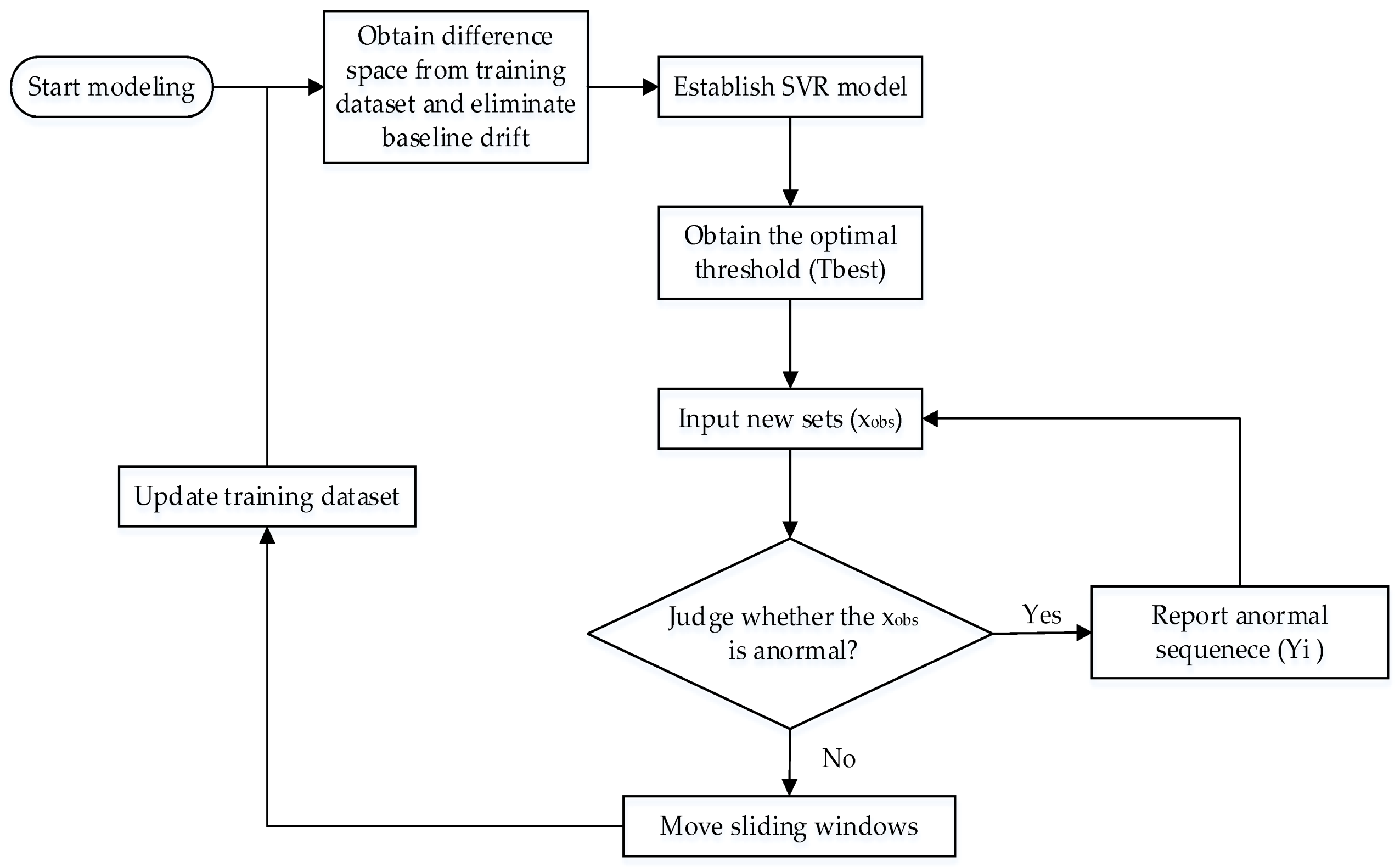
• The difference space is estimated from the normal sets in the training dataset and the latest normal sets in the test dataset, which has the same number of sets as the training dataset.
• The baseline drift of the training dataset is omitted by using the difference space obtained in Step 1. Then, the SVR model is established by adopting the labeled training dataset.
• The ROC curve is based on the detection rate of the ordinate and the FAR of the abscissa. The optimal threshold ($T_{best}$) is obtained according to the ROC curve.
• The test dataset is inputted with 50 UV-Vis spectral sets at each time. The baseline drift is removed from the new sets using the difference space obtained in Step 1. Then, the trained SVR method regresses the new sets and outputs the results. The outlier is obtained by comparing with the optimal threshold ($T_{best}$) determined using Step 3.
• Sequential Bayesian is used to identify outliers and determine contamination events. If no contamination event occurs, then the sliding window moves forward, and the procedure returns to Step 1. Otherwise, the program triggers the alarm signals and returns to Step 4.

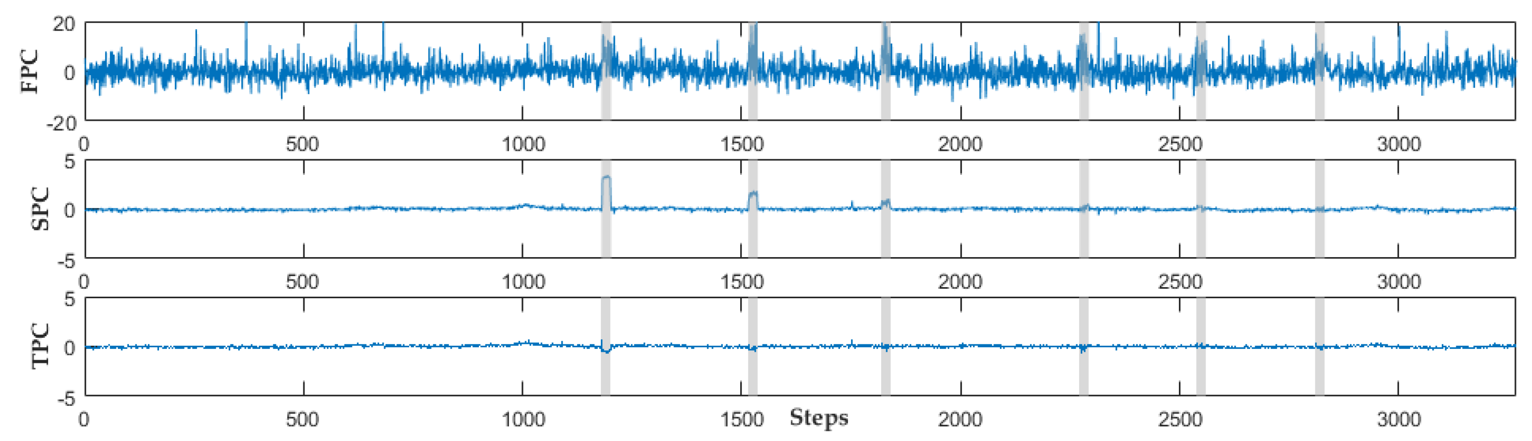
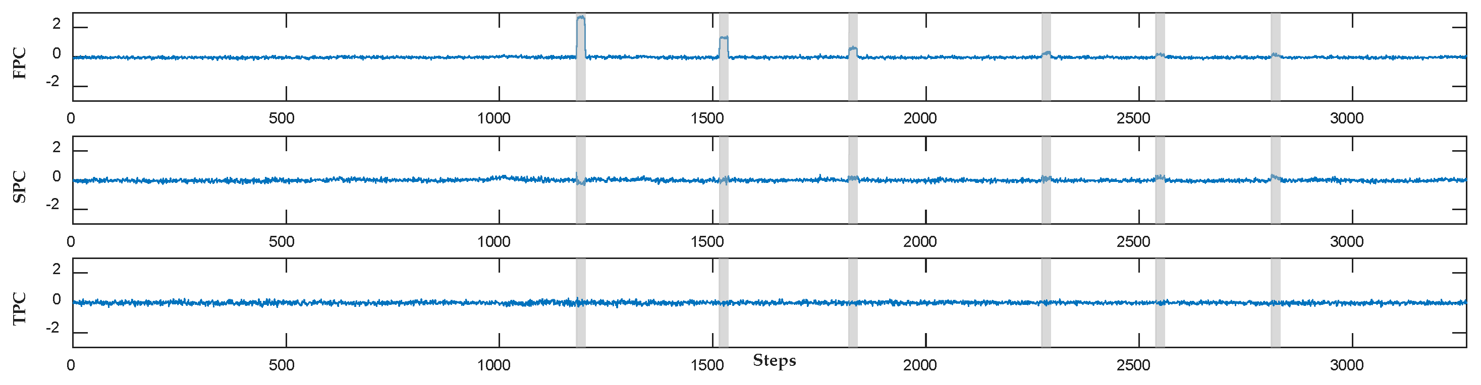
2.1. Dynamic Orthogonal Projection Correction

The orthogonal projection correction method removes the difference among various spectral data for preprocessing and denoises spectral data [20,21]. The spectral data observed at time $i$ is characterized by $x_{i,obs},i=1\dots N$, where $N$ is the observation duration and $x_{i,obs}$ is a row vector of multiple parameters. $x_{i,obs}$ is composed of two superimposed parts: the pure spectrum $x_i$ and the unexpected part $h_i$. It can be expressed as the following equation:

$$x_{i,obs}=x_i+h_i.$$

(1)

If the unexpected part $h_i$ of (1) is estimated correctly, then the pure spectrum can be characterized as

$$x_i=x_{i,obs}-h_i.$$

(2)

The cause of the unexpected part of each factor is complex. Hence, the distribution of each factor is difficult to estimate. Accordingly, an overall estimation of the unexpected part should be obtained instead. If space ${\epsilon }^D$ is used to characterize the spectral difference according to the orthographic projection theorem, then the corrected spectrum $x_{i,corr}$ can be expressed as a part of the original spectrum. In this manner, the components in the difference space are removed, thereby leaving the part in the zero space as the corrected value. Therefore, the corrected spectrum $x_{i,corr}$ can be represented by (3), where matrix $\mathrm{A}$ is a set of bases that characterize the difference space of the spectra ${\epsilon }^D$:

$$x_{i,corr}=x_{i,obs}{P}^{\perp }=x_{i,obs}(I-A^{⊺}{(A{A}^{⊺})}^{-1}A).$$

(3)

Orthogonal projection is used to remove the baseline drift through the difference space. The UV-Vis spectrum changes with the environment. Thus, baseline fluctuations lead to a decrease, or even a failure, in the ability of the orthogonal projection to perform baseline corrections. The core of the method, i.e., dynamic orthogonal projection correction, constantly searches for difference spaces in the training set by using the normal water quality data in a sliding window. Each time a difference space is found, orthogonal projection correction is applied to the training set and the newly obtained data to eliminate baseline drift.

2.2. SVR

SVR [22,23] replaces the linear term in traditional linear equations with a kernel function and constructs a linear decision function in high-dimensional space for prediction. A linear kernel function is used to map the input data onto a high-dimensional feature space $F$ (typically an infinite dimension). Then, linear regression is performed on the feature space. The estimation function is given by the following equation:

$$f(x)=\omega \cdot \phi (x)+b,$$

(4)

where $\phi :R^d\to F$ is mapped onto the feature space; and $\langle \cdot \rangle$ denotes the inner product in the feature space, $\omega \in F$ and $b\in R$. Given a dataset $\left\{(x_i,y_i),i=1,2,\dots n\right\}$ with a sample size of n, SVR obtains a regression function model of (4) to ensure that $f(x_i)$ and $y_i$ are as close as possible. Considering the characteristics of the spectral data, this study uses a $\epsilon -\mathrm{SVR}$ regression algorithm, which can be formalized as

$$\underset{\omega ,b}{\min }\frac{1}{2}{\left|\left|\omega \right|\right|}^2+C{{\displaystyle \sum }}_{i=1}^n{l}_{\epsilon }(f(x_i)-y_i),$$

(5)

where $C$ is regularization constant, and $l_{\epsilon }$ is an $\mathsf{\epsilon }-$ insensitive loss function. The obtained result of $\omega$ can be expressed as follows by solving the quadratic programming problem to minimize the regularization risk functional:

$$\omega ={{\displaystyle \sum }}_{i=1}^n(a_i^{*}-a_i)\phi (x_i).$$

(6)

The coefficients $a_i^{*},a_i\in R$ are determined by solving quadratic programming problems. Therefore, the estimation function presents the following equation:

$$f(x)={{\displaystyle \sum }}_{i=1}^n(a_i^{*}-a_i)K(x_i,x_j)+b,$$

(7)

where $K(x_i,x_j)$ is a kernel function.

In the modeling, SVR sets 0 as a normal sample and 1 as an abnormal sample. After obtaining the model, the optimal threshold is determined on the basis of the ROC curve of the training dataset. The SVR model is expressed as $f(\cdot )$. The alarm signal, which is the output at time $i$, is represented by $Y_i$. Thus, the outlier prediction result is the output at time $i$.

$$Y_i=\{\begin{array}{c}\text{“}\mathrm{Outlies}\text{”},y_i=f(x_{i,corr})\ge T_{best}\\ \text{“}\mathrm{Normal}\text{”},y_i=f(x_{i,corr})<T_{best}\end{array}$$

(8)

The output is the binary time series of 0 and 1, which is consistent with the SVR modeling process. 0 represents the normal point, whereas 1 denotes the outlier in the time series.

2.3. Sequential Bayesian Anomaly Detection

Many outliers still do not belong to the anomaly even after removing the baseline drift due to noise interference from the original data and other factors. In general, the abnormal outliers from the pollutant intrusion event will continue for several detection cycles because pollutant intrusion events last for a certain period. Therefore, the appearance of multiple continuous outliers is common in contamination events.

In this study, sequential water quality anomaly points are detected as events by using a sequential Bayesian update probability method [24,25,26]. In our time series analysis, the probability that a current point is an outlier is determined by historical observation points. Then, the state obtained by performing the sequential Bayes method at time $t+1$ is determined using the Bayesian equation:

$${\pi }_1(t+1)=\frac{{\pi }_{1}P(y_{t+1}|{\theta }_1)}{(1-{\pi }_1(t))P(y_{t+1}|{\theta }_0)+{\pi }_1(t)P(y_{t+1}|{\theta }_1)},$$

(9)

where ${\pi }_1(t)$ denotes the probability that t is anomalous, and the initial moment can be considered a small probability. Therefore, ${\pi }_1(0)$ is a small value. In our experiment, we set ${10}^{-5}$. We use (9) to obtain a probability that represents the possibility of an anomaly and then pass it to the next moment. If the probability ${\pi }_1(t+1)$ exceeds 0.95, then the current point is an abnormal point and set as an alarm. If the probability is lower than 0.95, then the point is a normal condition and set as unalarmed. In (9), ${\theta }_1$ is abnormal and ${\theta }_0$ is normal. $P(y_{t+1}|\theta )$ can be estimated on the basis of the detection or the FAR of the historical or training data at the optimal threshold point position.

2.4. ROC Curve

The ROC curve [27,28,29] is based on the detection rate of the ordinate and the FAR of the abscissa. The performance curve of the detection model is judged intuitively. In the same spectral dataset, we compare the performance of two or more detection models using the area under ROC (AUROC) [29]. In general, 0.5 < AUROC < 1. Hence, the greater the AUROC, the better the performance. The same water quality detection model considers that the higher the detection rate, the lower the FAR, and consequently, the better the detection result. Thus, the threshold value that is represented by the point closest to the upper left corner on the ROC curve is a balance point. This point can be considered the optimal threshold ($T_{best}$) of the model.

2.5. Detection Accuracy

The performance evaluation indexes of abnormal water quality detection methods typically include the true positive rate (TPR) and FAR [30]. The TPR is the percentage of the total number of organic contamination events detected by the method within a certain period. It can be formalized as (10). The FAR is the percentage of false water quality contamination events detected by the algorithm within a certain period. It can be formalized as (11).

$$\mathrm{TPR}=\frac{\mathrm{TP}}{\mathrm{TP}+\mathrm{FN}},$$

(10)

$$\mathrm{FAR}=\frac{\mathrm{FP}}{\mathrm{FP}+\mathrm{TN}},$$

(11)

The meanings of TP, TN, FP, and FN are provided in

Table 1. The meaning of TP, TN, FP, FN.

	Real Class	Normal	Abnormal
Predict Class
Normal		True Negative (TN)	False Negative (FN)
Abnormal		False Positive (FP)	True Positive (TP)

. The higher the calculated TPR value, the better the detection performance. The higher the calculated FAR value, the worse the detection performance.

3. Experiments and Results

This section, which includes the introduction of experiments and the analysis of results, is organized as follows. In Section 3.1, the experimental device and procedures are described (Section 3.1.1), and the organic contaminants and experimental datasets are implemented (Section 3.1.2). Section 3.2 presents the detection results of the semi-supervised learning model (Section 3.2.1), the supervised learning model (Section 3.2.2), and the unsupervised learning model (Section 3.2.3). Finally, the analysis results (Section 3.2.4) indicate that the semi-supervised learning model achieves the best performance in detecting organic contamination events.

3.1. Experimental Data Acquisition

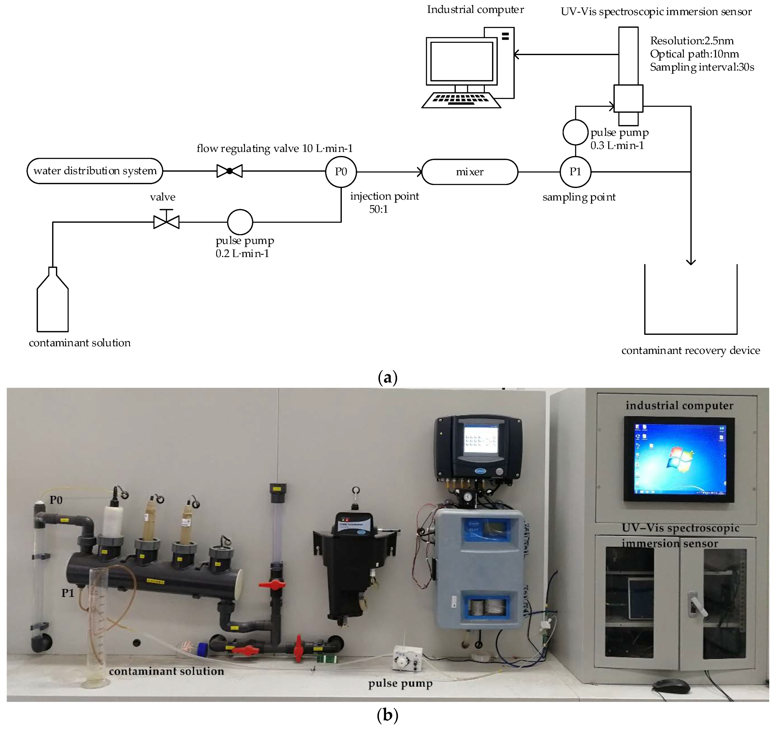
3.1.1. Experiment Device Introduction

The core of testing the developed methodology is to create simulated organic contamination events in water distribution systems and attempt to detect them using a UV-Vis spectrometer. The experimental platform for detecting organic contamination events in urban drinking water comprises a water distribution pipe and a UV-Vis spectrometer connected to an actual water distribution system (Figure 2). An industrial computer that controls the water quality monitoring process and saves the UV-Vis spectral data is embedded into the system. The pipeline of the experimental setup is made of unplasticized polyvinyl chloride with a length of 6 m and an internal diameter of 1.50 cm. Organic contamination events are simulated by injecting an organic contaminant solution into the pipeline (P0) using a high-frequency pulse pump. A mixing pipe thoroughly mixes the organic contaminant solution with the urban drinking water to ensure that the contaminant intrusion event achieves a uniform concentration distribution. After mixing uniformly, the contaminant solution is extracted from the pipeline (P1) using a pulse pump. Then, the contaminant solution flows through the UV-Vis spectroscopic immersion sensor with an immersed path length of 10 mm spectrometer.

Before the simulation of organic contamination events, the experimental platform runs for a certain period (>1 h) to obtain a sufficient baseline of normal water quality. The baseline of normal water quality is used to establish the difference space of dynamic orthogonal projection when the semi-supervised model is first trained. Simultaneously, various concentrations of different contaminant solutions supplied with tap water are prepared to verify the feasibility of the developed methodology.

During the simulation of organic contamination events, the regulation flow in the experimental device is 10 L∙min⁻¹. The interval between events should be sufficiently long (>1 h) to eliminate interference. A standard concentration of the contaminated solution is injected into the static mixing tube through a pulse pump. The injected flow rate is controlled by the closed-loop feedback system that controls the pulse pump. The flow is fine-tuned to reflect the pipeline. In this manner, the dosing flow rate is stabilized at 0.2 L∙min⁻¹. The ratio of the injected pollutant flow to the pipeline flow is 1:50. The flow time of the contaminants from the injection point (P0) to the sampling point (P1) is approximately 11.67 s. The spectrometer performs measurement every 30 s. The measurement and delay times are 20 s and 10 s, respectively. The real-time scanning wavelength range of the UV-Vis sensor is 200–750 nm, and the resolution is 2.5 nm. In this study, the wavelength range of the selected set is 240–400 nm.

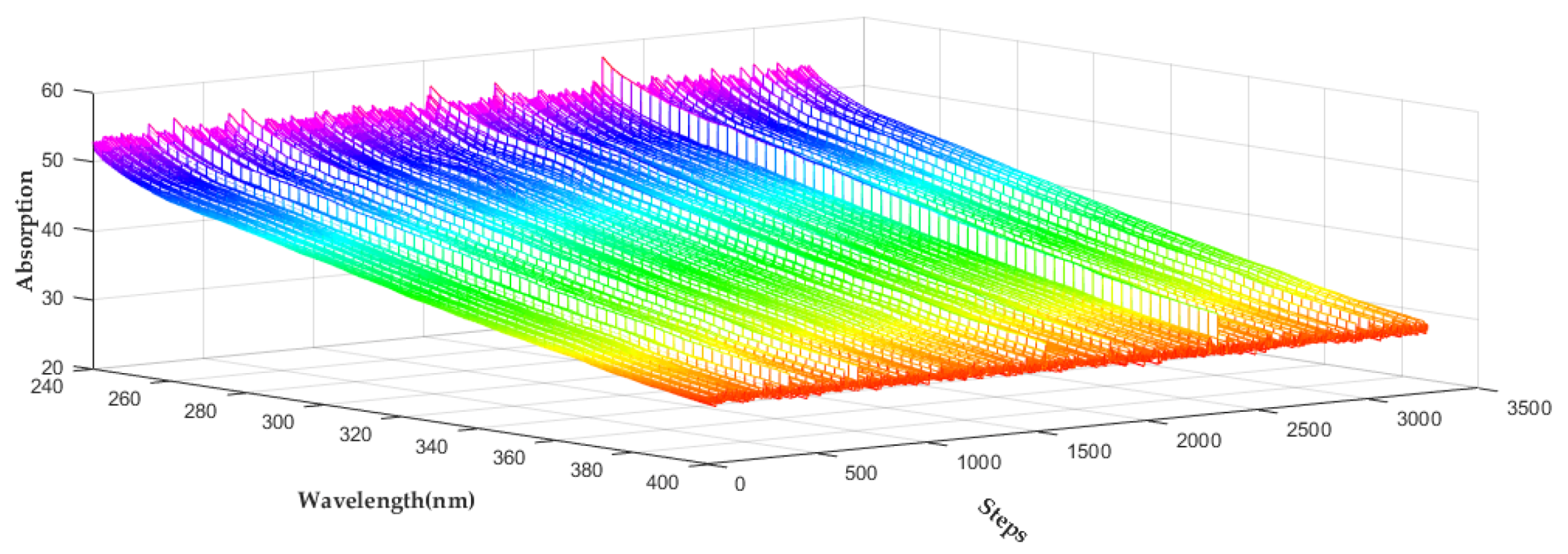
3.1.2. Organic Contaminant Selection and Dataset Acquisition

Organic contaminants are major threats to water distribution systems because they affect the safety of drinking water [13,14,15,16]. Several organic aromatic compounds exhibit fingerprint characteristics for the UV-Vis spectrum. Four types of typical organic contaminants, namely, phenol, m-phenylenediamine, hydroquinone, and resorcinol, are selected in the experiment. Phenol is an organic contaminant listed in the 2012 Edition of the Drinking Water Standards and Health Advisories (US Environmental Protection Agency 2012). Phenol is a high-risk organic aromatic compound, and its significant absorption peaks are at 270 nm and 290 nm. To verify that the detection method is feasible for other organic pollutants, m-phenylenediamine, hydroquinone, and resorcinol are selected as representatives. The three pollutants are frequently used in the chemical industry and exhibit their own absorption peaks. The four substances are frequently detected in water distribution systems and dangerous if consumed even in minimal amounts. Hence, they are selected in the experiment to create simulated contamination events.

The study is based on datasets that contain normal water quality and organic contamination events recorded from March to April 2017. Each organic contamination event corresponds to different concentration intensities of 20, 30, 40, 50, 100, and 200 µg·L⁻¹. The dilution ratio is 1:50. Therefore, the concentrations of the injected solution are 1, 1.5, 2.0, 2.5, 5, and 10 mg·L⁻¹. The interval among events is greater than 1 h, and each event lasts approximately 20 steps. To verify the feasibility of the semi-supervised learning method, experiments with varying concentrations (20, 30, 40, 50, 100, and 200 µg·L⁻¹) of different pollutants (phenol, m-phenylenediamine, hydroquinone, and resorcinol) are conducted twice at various times. One experiment is used as a training dataset, whereas the other is used as a test dataset. In this study, the wavelength range of the selected UV-Vis spectral data is 240–400 nm. The resolution of the original spectrum is 2.5 nm. Hence, each UV-Vis spectral set includes 65 points that represent the absorption values of the corresponding wavelength. Figure 3 shows the portion of the data sampled in the experiment, with phenol as an example. Although six organic contamination events are injected, the locations of the events are not evident due to the influence of baseline drift.

3.2. Detection Results of Organic Contamination Events

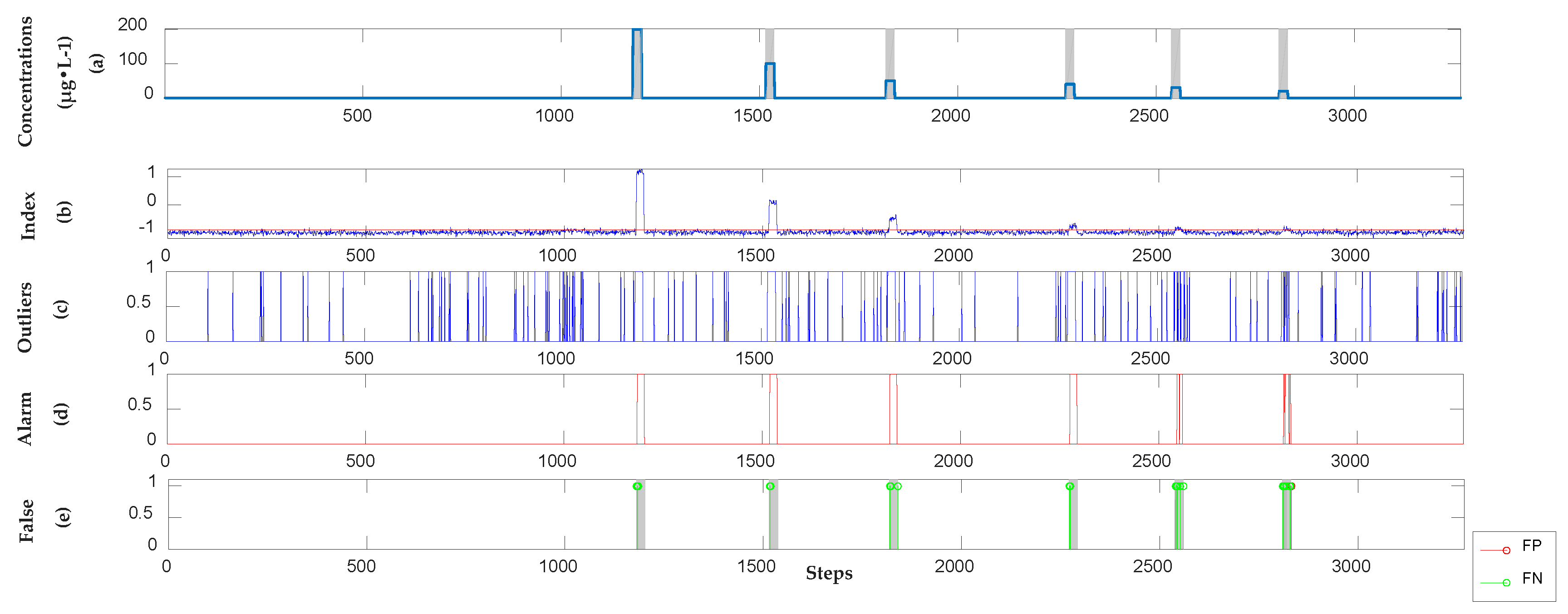
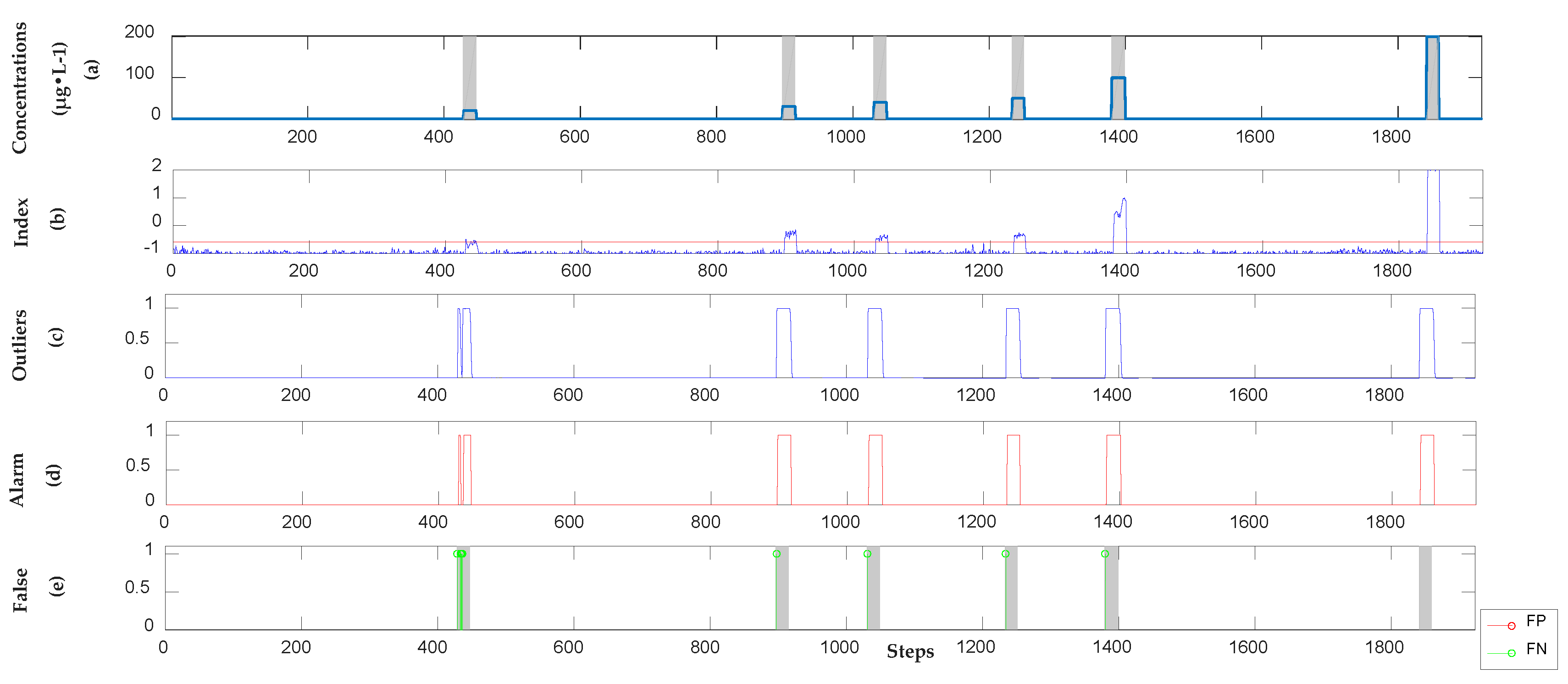
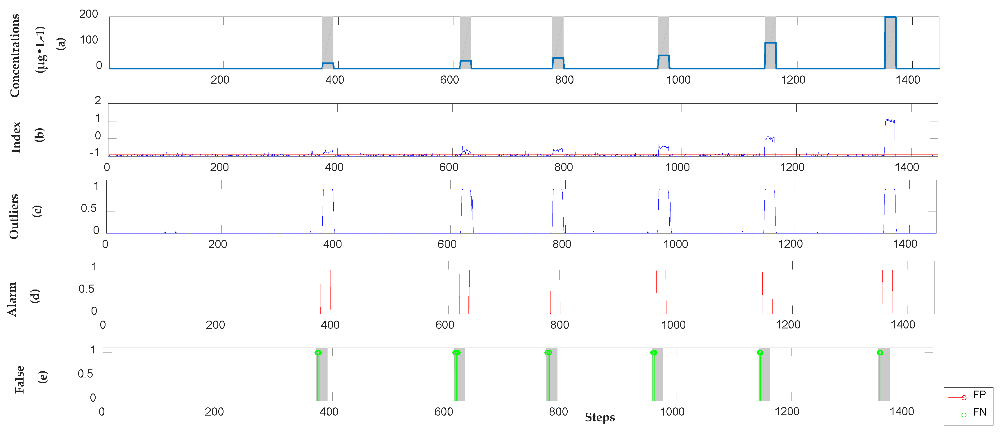
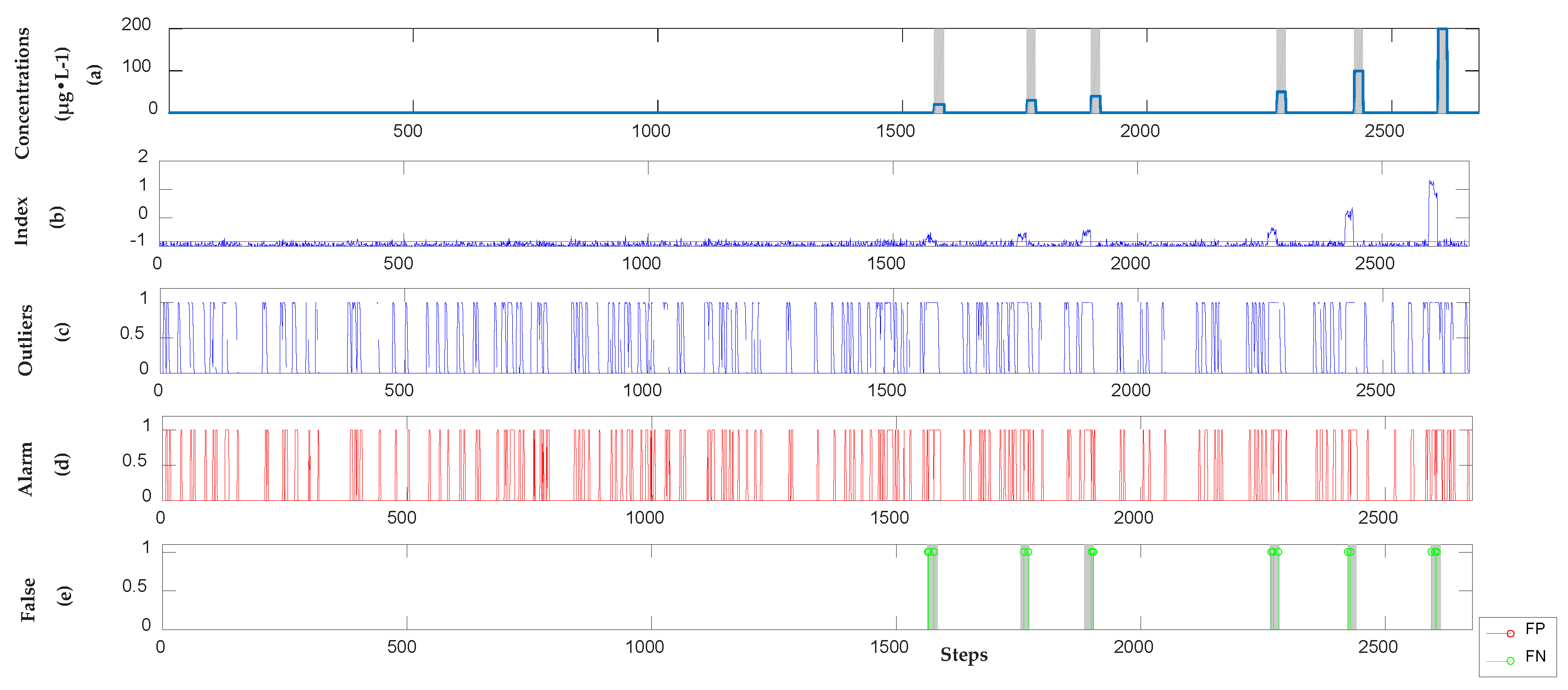
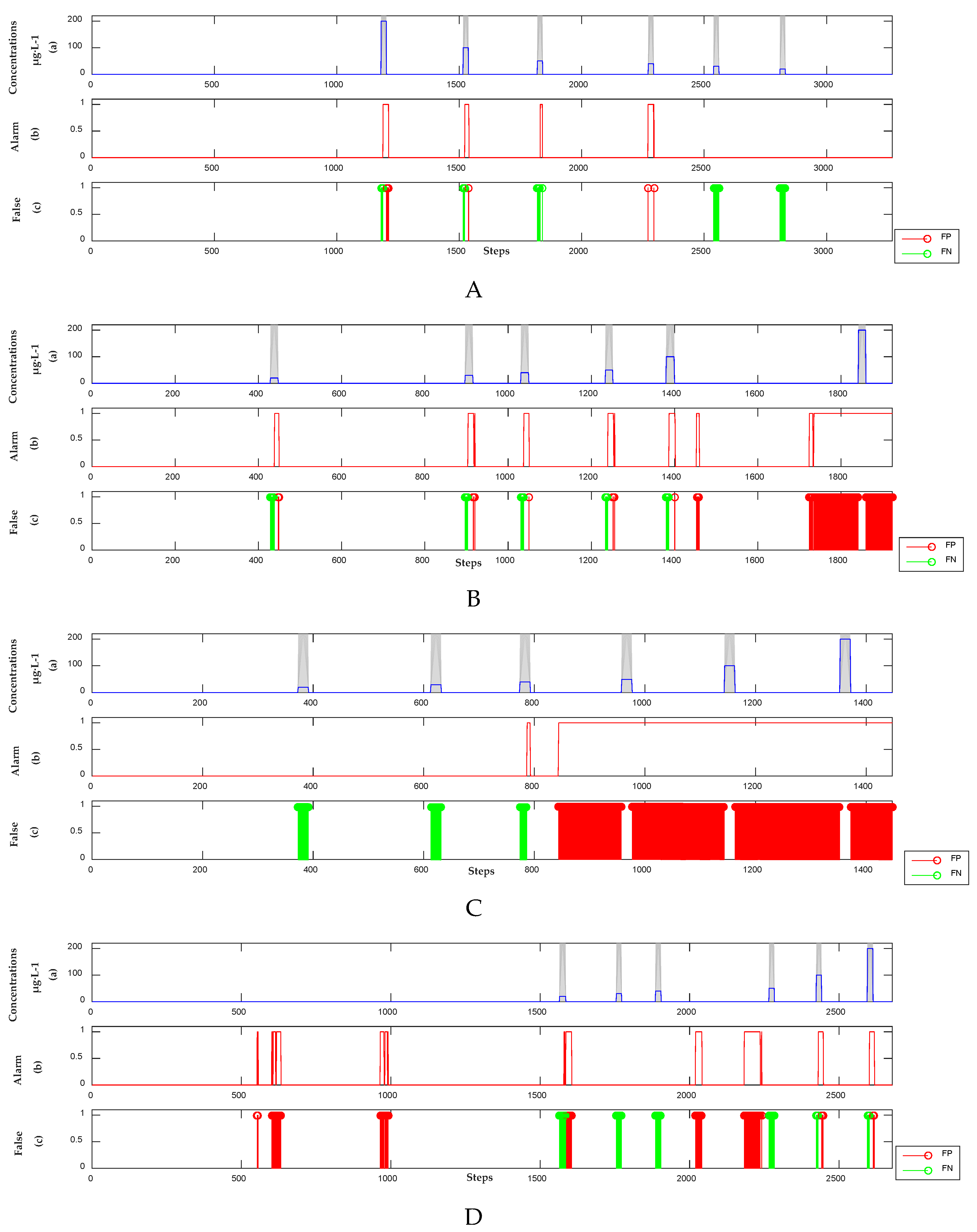
3.2.1. Detection Results of Semi-Supervised Learning Model

Considering the full use of prior knowledge and the dynamic baseline drift of the spectrum, the detection method for organic contamination events in water distribution systems based on semi-supervised learning is modeled according to Figure 1. The corresponding semi-supervised learning model is obtained by training the dataset of the four organic contaminants. The training dataset of each organic contaminant includes different concentrations (20, 30, 40, 50, 100, and 200 µg·L⁻¹) of organic contaminant and normal water quality data. The area under ROC (AUROC) and optimal threshold ($T_{best}$) (Section 2.4) of the corresponding model for each organic contaminant are shown in

Table 2. Parameters of semi-supervised model for different contaminants.

Organic Contaminant	AUROC	${\mathit{T}}_{\mathit{b}\mathit{e}\mathit{s}\mathit{t}}$
phenol	0.97440	−0.8131
m-phenylenediamine	0.96517	−0.5785
hydroquinone	0.96957	−0.8806
resorcinol	0.95730	−0.8310

. The ROC results of the training sets of different organic contaminants listed in Table 2 show that AUROC is close to 1. Thus, the semi-supervised learning model achieves excellent detection of each contaminant.

Four organic contaminants are identified after completing the semi-supervised learning model of each organic contaminant. The dynamic orthogonal projection correction method (3) is used to continuously update the difference space in a sliding window to dynamically correct the baseline and denoise the new sets. The trained SVR model (7) is applied to detect new sets for obtaining the alarm signals and determining the outliers via $T_{best}$ (8). Single-point false positives (FPs) are filtered using sequential Bayes (9), and successive alarm sequences are obtained. Figure 4, Figure 5, Figure 6 and Figure 7 present the detection results. In each figure, (a) indicates the location and concentration of each event; whereas (b) shows the probability of contamination events calculated using SVR. The threshold is obtained according to the model that corresponds to different organic contaminants. It is indicated as a red dotted line in (b) for triggering alarm signals during organic contamination events; (c) shows the anomaly outliers obtained using SVR; (d) presents the anomalous alarm triggered by the sequential Bayesian. The alarm triggered in (d) is accurate in determining the locations of organic contamination events; (e) illustrates the accuracy of the detection. FN indicates the false negative point, whereas FP indicates the false positive point.

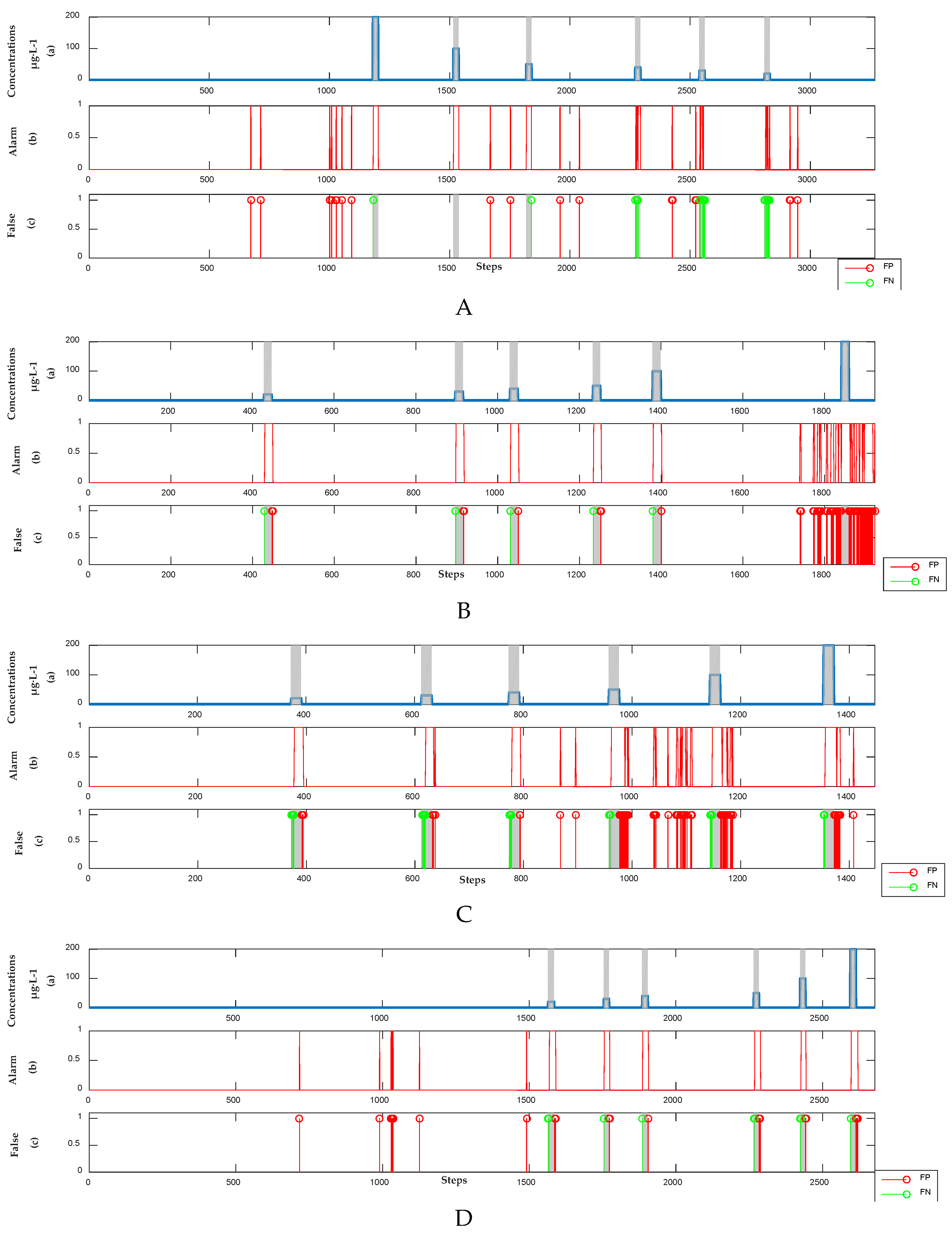
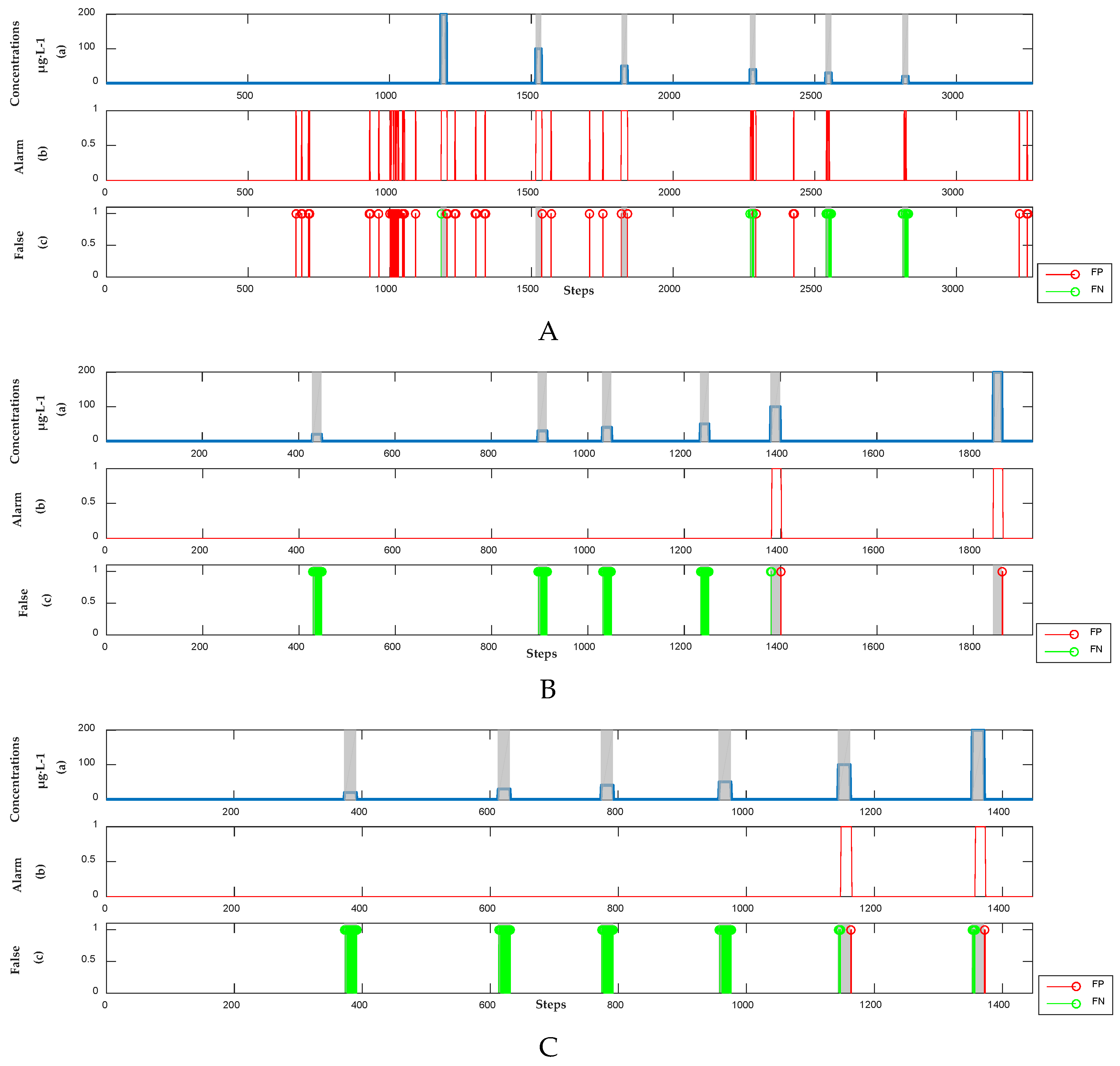
3.2.2. Detection Results of Supervised Learning Model

The baseline drift of UV-Vis spectral data changes with the environment (such as temperature and water flow rate), and the drift range is unpredictable. The supervised model obtains a model by learning the fixed labeled dataset [22,31,32,33]. Therefore, the model cannot be adapted to the baseline drift. To demonstrate this scenario, a supervised model is used to analyze the UV-Vis spectral data of phenol, m-phenylenediamine, hydroquinone, and resorcinol. The results are presented in Figure 8. The detection of contamination events has no false negative (FN) but has a large number of FPs. This large number occurs because the baseline changes considerably during detection, thereby exceeding the predictions for baseline change in the test dataset made by the orthogonal projection correction and estimated by the SVR model.

3.2.3. Detection Results of Unsupervised Model

In studying the unsupervised model [14], PCA is used to extract the principal components of the newly collected UV-Vis spectral data, whereas Hotelling’s T2 statistical method is adopted to calculate the principal components. If the result of the latter exceeds the threshold, then the point is an outlier. Finally, the outliers are filtered using sequential Bayes. As shown in Figure 9, the results of the unsupervised model have a large number of FNs and positives.

3.2.4. Analysis Results

Figure 4, Figure 5, Figure 6, Figure 7, Figure 8 and Figure 9 present the results of the three methods. The results of the semi-supervised learning model are provided in Figure 4, Figure 5, Figure 6 and Figure 7. All events can be detected without any FPs. The supervised model can detect all events. However, some FPs are observed, as shown in Figure 8. In Figure 9, the unsupervised model is ineffective in detecting events with concentrations below 50 µg·L⁻¹. Moreover, several FPs are identified. In particular,

Table 3. Comparison of three methods based on the points’ level.

	Unsupervised		Supervised		Semi-Supervised
Organic Contaminants	TPR	FAR	TPR	FAR	TPR	FAR
phenol	0.4545	0.0041	0.7652	0.0096	0.7576	0.0001
m-phenylenediamine	0.6726	0.1094	0.9558	0.0514	0.9204	0
hydroquinone	0.5526	0.4144	0.7544	0.0555	0.7368	0
resorcinol	0.2212	0.0624	0.8673	0.0129	0.8584	0

shows the TPR (10) and FAR (11) of the four organic contamination events based on the level of points. The average accuracy of the supervised model, which reaches approximately 80%, is the highest among the three methods but accompanied by a small number of FPs. However, when measuring performance at the level of the contamination event (it is considered the same event if the interval between points does not exceed 3), true positive (TP) is the detection of an actual event, whereas FP refers to normal water quality data being incorrectly classified as a contamination event.

Table 4. Comparison of three methods based on the events’ level. (Each organic contaminant includes 6 events). TP indicates the number of abnormal events detected; FP indicates the number of false positive events.

	Unsupervised		Supervised		Semi-Supervised
Organic Contaminants	TP	FP	TP	FP	TP	FP
phenol	4	0	6	14	6	0
m-phenylenediamine	6	4	6	8	6	0
hydroquinone	1	1	6	11	6	0
resorcinol	3	7	6	4	6	0

shows the TP and FP of the four organic contaminant events based on the level of the events. The semi-supervised learning model can detect all organic contamination events without any false positives, and the TP and FP of this model are considerably better than those of the supervised and unsupervised learning models.

An event typically contains a series of consecutive points. Hence, the level of the contamination event should be used to judge detection performance. Compared with the results of the supervised and unsupervised learning models, the accuracy of the semi-supervised learning model is considerably improved. The semi-supervised model dynamically eliminates baseline drift and uses unlabeled data to dynamically correct such drift. In this manner, a large number of FPs in the supervised and unsupervised models are eliminated. Hence, the semi-supervised learning model can effectively detect organic contamination events without any FPs. However, a small number of FN points and positive negative points still occur in each event. In conclusion, compared with the unsupervised model, the supervised learning model can effectively reduce the detection limit of organic contaminants. Moreover, the semi-supervised learning model exhibits better adaptability and performance in detecting organic contamination events than the supervised learning model.

4. Discussion

The effect of dynamic orthogonal projection correction and the adaptability of the semi-supervised learning model when the baseline gradually drifts are discussed in this paper. First, the comparison of the effects of baseline drift correction with dynamic orthogonal projection correction and without baseline drift correction shows that the former can effectively eliminate baseline drift and improve the signal-to-noise ratio (SNR). Second, the comparison of the detection accuracy of the supervised and semi-supervised models when the baseline gradually drifts indicates that the latter can adapt to the baseline drift more effectively than the former.

4.1. Effect of Dynamic Orthogonal Projection Correction

UV-Vis spectral data changes with time. Thus, the spectral dataset collected at different times has varying ranges of drift. The interference of baseline drift on the training and test datasets should be reduced [14,15,16]. If the raw data are modeled directly, then the detection results generate a large number of FPs and negatives. To adapt to the dynamic changes of the spectrum and extract useful signals, dynamic orthogonal projection correction is continuously used in eliminating baseline drift.

To clearly illustrate the interference of baseline correction, the UV-Vis spectral sets of phenol are used as example. As shown in Figure 3, approximately 3300 UV-Vis spectral sets of phenol are collected, including 6 organic contamination events. The organic contamination events are difficult to analyze because of the high dimension of the original UV-Vis spectral sets and baseline drift. To intuitively demonstrate changes in the UV-Vis spectral data, PCA can effectively reduce the dimension of UV-Vis spectral data and extract features. The dimension and features of the data are reduced and extracted, respectively, using PCA. Then, the change in the UV-Vis spectral data can be observed clearly. The first to third principal components of the original UV-Vis spectral data of phenol are shown in Figure 10. Meanwhile, Figure 11 presents the first to third principal components of the UV-Vis spectral data of phenol corrected via dynamic orthogonal projection.

Figure 10 shows that the phenol invasions in the first principal component, which represent 98.88% of the information of the UV-Vis spectrum, are submerged by the baseline drift. Although the second and third principal components can clearly express three phenol invasion events, they only represent 0.49% and 0.11%, respectively. The results of the UV-Vis spectral data corrected by dynamic projection correction are presented in Figure 11. The first to third principal components of the UV-Vis spectral sets of phenol corrected by dynamic orthogonal projection represent 42.96%, 9.76%, and 7.35%, respectively. The abnormal changes in the first principal component of the UV-Vis spectral data at the points where phenol intrudes are clearly more recognizable than those in Figure 10. Therefore, the signals of organic contamination events are amplified after correcting the baseline drift via dynamic orthogonal projection.

To demonstrate the effect of dynamic baseline correction, we construct the semi-supervised learning model directly from the UV-Vis spectral sets of phenol, m-phenylenediamine, hydroquinone, and resorcinol. The results are presented in Figure 12 and

Table 5. Comparison the two methods based on the events’ level (Each organic contaminant includes 6 events). TP indicates the number of abnormal events detected; FP indicates the number of false positive events.

	Baseline Correction		No Baseline Correction
Organic Contaminants	TP	FP	TP	FP
phenol	6	0	6	17
m-phenylenediamine	6	0	2	0
hydroquinone	6	0	2	0
resorcinol	6	0	6	0

. When compared with Figure 4, Figure 5, Figure 6 and Figure 7, the detection results of the organic contamination events contain FPs apart from a large number of FNs.

Therefore, eliminating baseline drift through dynamic orthogonal projection can considerably improve SNR and reduce the impact of water quality fluctuations, thereby subsequently increasing detection accuracy.

4.2. Comparison of the Adaptability between the Supervised and Semi-Supervised Models When the Baseline Gradually Drifts

To study the adaptability of the detection methods using the UV-Vis spectrum, the practical problems of the long-term situation of water quality monitoring with the baseline slowly drifting should be solved. We collect more than 63,000 UV-Vis spectral datasets of water quality within 23 days. Three incidents of m-phenylenediamine events are injected at different time intervals. Each event includes concentration intensities of 20, 30, 40, 50, 100, and 200 µg·L⁻¹. These intensities are used to analyze event detection in long-term situations. PCA is used to obtain the first to third principal components of the UV-Vis spectral data for depicting the baseline drift, as shown in Figure 13. If the dashed line is used to divide the daily monitoring data, then the baseline is shown to gradually drift.

A supervised learning model is used to analyze the UV-Vis spectral sets observed over the previous 23 days. The results are presented in Figure 14. The alarm signals for the test dataset obtained with the supervised learning model also drifts to a certain extent due to the drift on the surface of the water quality baseline. Figure 14b shows that the alarm results for SVR gradually deviate below the threshold, thereby rendering the optimal threshold obtained in the training dataset invalid in the test dataset. Meanwhile, a semi-supervised model is also applied to analyze the same UV-Vis spectral sets. The orthogonal projection and SVR models are updated using unlabeled sets. The results are provided in Figure 15. Figure 15b shows the SVR output for the alarm signals, whereas Figure 15c presents the outliers obtained after comparing the alarm information with the optimal threshold ($T_{best}$) of the training dataset. Sequential Bayesian is used to update the probability of outliers. When the probability threshold exceeds 0.95, a contamination event has occurred. The result is recorded in the water quality alarm sequence, as shown in Figure 15d. Compared with the detection results of the supervised learning model, the semi-supervised learning model can detect events effectively when the baseline gradually drifts.

Therefore, the semi-supervised learning method can more effectively adapt to baseline drift than the supervised learning model. The semi-supervised learning model can detect all organic contamination events, whereas the supervised model becomes gradually invalid with baseline drift. The supervised model trains a model by learning the fixed labeled dataset that does not cover all the cases of the baseline drift. Thus, the detection accuracy of the supervised model is comparatively low in the tests. To adapt to the gradual drift of the baseline, the semi-supervised learning model maximizes the information from the labeled and new data. Then, it dynamically updates the anomaly detection model, thereby possibly improving the detectability of organic contamination events using the UV-Vis spectrum to a considerable extent.

5. Conclusions

This study presents a novel method that combines dynamic orthogonal projection correction and an SVR model to detect organic contamination events in water distribution systems.

The proposed semi-supervised learning method adopts a dynamic orthogonal projection correction method to continuously update the difference space. In this manner, the incapability of static orthogonal projection correction to adequately adapt to the baseline drift is overcome. After eliminating the baseline drift via dynamic orthogonal projection, the signals of the organic contamination events are highlighted. This method processes unlabeled samples and maximizes the implicit supervision information provided by the samples of the labeled dataset. It also fully uses unlabeled data and considerably improves the detectability of organic contamination events with the UV-Vis spectrum. The semi-supervised learning model dynamically updates the orthogonal projection correction and the SVR model. Accordingly, the method can provide accurate detection even when the baseline drifts considerably.

Despite the advantages of the detection method, a certain number of FN points still occur in the organic contamination events, particularly when the concentration is below 30 µg·L⁻¹. Additional studies should be conducted in the future to further reduce the FN points. By purposefully extracting features from the UV-Vis spectral data, the signals of low-concentration organic contaminants can be amplified, particularly to enhance detection performance when the concentration is below 30 µg·L⁻¹.

Therefore, the proposed method can effectively detect organic contaminants by evaluating UV-Vis spectral sets. This novel method can be applied to water distribution systems to ensure the safety of drinking water given its high adaptability and good performance.

References

1. Piao, S.; Ciais, P.; Huang, Y.; Shen, Z.; Peng, S.; Li, J.; Zhou, L.; Liu, H.; Ma, Y.; Ding, Y.; et al. The impacts of climate change on water resources and agriculture in China. Nature 2010, 467, 43–51. [Google Scholar] [CrossRef] [PubMed]
2. Hasan, J.; States, S.; Deininger, R. Safeguarding the security of public water supplies using early warning systems: A brief review. J. Contemp. Water Res. Educ. 2004, 129, 27–33. [Google Scholar] [CrossRef]
3. Conde, E.F. Environmental Sensor Anomaly Detection Using Learning Machines; Utah State University: Logan, UT, USA, 2011. [Google Scholar]
4. Kühnert, C.; Baruthio, M.; Bernard, T.; Steinmetz, C.; Weber, J. Cloud-based event detection platform for water distribution networks using machine-learning algorithms. Procedia Eng. 2015, 119, 901–907. [Google Scholar] [CrossRef]
5. Hou, D.; He, H.; Huang, P.; Zhang, G.; Loaiciga, H. Detection of water-quality contamination events based on multi-sensor fusion using an extented dempster-shafer method. Meas. Sci. Technol. 2013, 24, 055801. [Google Scholar] [CrossRef]
6. Liu, S.; Che, H.; Smith, K.; Lei, M.; Li, R. Performance evaluation for three pollution detection methods using data from a real contamination accident. J. Environ. Manag. 2015, 161, 385–391. [Google Scholar] [CrossRef] [PubMed]
7. Liu, S.; Smith, K.; Che, H. A multivariate based event detection method and performance comparison with two baseline methods. Water Res. 2015, 80, 109–118. [Google Scholar] [CrossRef] [PubMed]
8. Huang, P.; Yu, J.; Hou, D.; Yu, J.; Tu, D.; Cao, Y.; Zhang, G. Online classification of contaminants based on multi-classification support vector machine using conventional water quality sensors. Sensors 2017, 17, 581. [Google Scholar] [CrossRef] [PubMed]
9. Langergraber, G.; Weingartner, A.; Fleischmann, N. Time-resolved delta spectrometry: A method to define alarm parameters from spectral data. Water Sci. Technol. 2004, 50, 13–20. [Google Scholar] [PubMed]
10. Langergraber, G.; Fleischmann, N.; Hofstaedter, F. A multivariate calibration procedure for uv/vis spectrometric quantification of organic matter and nitrate in wastewater. Water Sci. Technol. 2003, 47, 63–71. [Google Scholar] [CrossRef] [PubMed]
11. Guercio, R.; Di Ruzza, E. An early warning monitoring system for quality control in a water distribution network. WIT Trans. Ecol. Environ. 2007, 103, 143–152. [Google Scholar]
12. Dürrenmatt, D.J.; Gujer, W. Identification of industrial wastewater by clustering wastewater treatment plant influent ultraviolet visible spectra. Water Sci. Technol. 2011, 63, 1153–1159. [Google Scholar] [CrossRef] [PubMed]
13. Hou, D.; Zhang, J.; Yang, Z.; Liu, S.; Huang, P.; Zhang, G. Distribution water quality anomaly detection from UV optical sensor monitoring data by integrating principal component analysis with chi-square distribution. Opt. Express 2015, 23, 17487–17510. [Google Scholar] [CrossRef] [PubMed]
14. Zhang, J.; Hou, D.; Wang, K.; Huang, P.; Zhang, G.; Loaiciga, H. Real-time detection of organic contamination events in water distribution systems by principal components analysis of ultraviolet spectral data. Environ. Sci. Pollut. Res. 2017, 24, 12882–12898. [Google Scholar] [CrossRef] [PubMed]
15. Guo, B.; Hou, D.; Jin, Y.; Yin, H.; Huang, P.; Zhang, G.; Zhang, H. Online detecting water quality anomaly from UV/Vis spectra using baseline correction and principal component analysis method. Spectrosc. Spectr. Anal. 2017, 37, 1460–1465. [Google Scholar]
16. Yin, H.; Yu, Q.; Dong, H.; Hou, D.; Huang, P.; Zhang, G. Detection of specific contamination events in water distribution system using ultraviolet spectra. In Proceedings of the 2018 IEEE International Instrumentation and Measurement Technology Conference (I2MTC), Houston, TX, USA, 14–17 May 2018. [Google Scholar] [CrossRef]
17. Huang, G.; Song, S.; Gupta, J.N.; Wu, C. Semi-supervised and unsupervised extreme learning machines. IEEE Trans. Cybern. 2017, 44, 2405–2417. [Google Scholar] [CrossRef] [PubMed]
18. Zhou, Z.H.; Li, M. Semi-supervised learning by disagreement. Knowl. Inf. Syst. 2010, 24, 415–439. [Google Scholar] [CrossRef]
19. Blanchard, G.; Lee, G.; Scott, C. Semi-supervised novelty detection. J. Mach. Learn. Res. 2010, 11, 2973–3009. [Google Scholar]
20. Boulet, J.C.; Roger, J.M. Pretreatments by means of orthogonal projections. Chemom. Intell. Lab. Syst. 2012, 117, 61–69. [Google Scholar] [CrossRef]
21. Poerio, D.V.; Brown, S.D. Dual-domain calibration transfer using orthogonal projection. Appl. Spectrosc. 2017, 72, 378–391. [Google Scholar] [CrossRef] [PubMed]
22. Hsu, C.W.; Lin, C.J. A simple decomposition method for support vector machines. Mach. Learn. 2002, 46, 291–314. [Google Scholar] [CrossRef]
23. Rivas-Perea, P.; Cota-Ruiz, J. An algorithm for training a large scale support vector machine for regression based on linear programming and decomposition methods. Pattern Recognit. Lett. 2013, 34, 439–451. [Google Scholar] [CrossRef]
24. Oliker, N.; Ostfeld, A. Comparison of multivariate classification methods for contamination event detection in water distribution systems. Procedia Eng. 2014, 70, 1271–1279. [Google Scholar] [CrossRef]
25. Aktekin, T.; Polson, N.; Soyer, R. Sequential bayesian analysis of multivariate count data. Bayesian Anal. 2018, 13, 385–409. [Google Scholar] [CrossRef]
26. Perelman, L.; Arad, J.; Housh, M.; Ostfeld, A. Event detection in water distribution systems from multivariate water quality time series. Environ. Sci. Technol. 2012, 46, 8212. [Google Scholar] [CrossRef] [PubMed]
27. Fawcett, T. An introduction to ROC analysis. Pattern Recognit. Lett. 2006, 27, 861–874. [Google Scholar] [CrossRef]
28. Metz, C.E. Basic principles of roc analysis. Semin. Nuclear Med. 1978, 8, 283–298. [Google Scholar] [CrossRef]
29. Hand, D.J.; Till, R.J. A simple generalisation of the area under the ROC curve for multiple class classification problems. Mach. Learn. 2001, 45, 171–186. [Google Scholar] [CrossRef]
30. Arad, J.; Housh, M.; Perelman, L.; Ostfeld, A. A dynamic thresholds scheme for contaminant event detection in water distribution systems. Water Res. 2013, 47, 1899–1908. [Google Scholar] [CrossRef] [PubMed]
31. Zhou, Z. Multi-instance learning from supervised view. J. Comput. Sci. Technol. 2006, 21, 800–809. [Google Scholar] [CrossRef]
32. Ye, X.; Wu, G.; Fan, F.; Peng, X.; Wang, K. Overhead ground wire detection by fusion global and local features and supervised learning method for a cable inspection robot. Sens. Rev. 2018, 38, 376–386. [Google Scholar] [CrossRef]
33. Zhou, Z. A brief introduction to weakly supervised learning. Natl. Sci. Rev. 2018, 5, 44–53. [Google Scholar] [CrossRef]
Figure 1. Modeling and detection flow chart.
Water 10 01566 g001
Figure 2. Detection device structure for an urban drinking-water pipe network. (a) Schematic Diagram; (b) Actual Experimental Installation Diagram.
Water 10 01566 g002
Figure 3. Original data of UV-Vis spectra of phenol.
Water 10 01566 g003
Figure 4. The detection results of phenol in the semi-supervised model. (a) Location and concentration of each event; (b) Alarm signals, which exceeded the threshold shown as the red dotted line; (c) Outliers obtained by using SVR; (d) Alarm sequences triggered by Sequential Bayesian; (e) False positive (FP) points and False negative (FN) points compare with real categories.
Water 10 01566 g004
Figure 5. The detection results of m-phenylenediamine in the semi-supervised model. (a) Location and concentration of each event; (b) Alarm signals, which exceeded the threshold shown as the red dotted line; (c) Outliers obtained by using SVR; (d) Alarm sequences triggered by Sequential Bayesian; (e) FP points and FN points compare with real categories.
Water 10 01566 g005
Figure 6. The detection results of hydroquinone in the semi-supervised model. (a) Location and concentration of each event; (b) Alarm signals, which exceeded the threshold shown as the red dotted line; (c) Outliers obtained by using SVR; (d) Alarm sequences triggered by Sequential Bayesian; (e) FP points and FN points compare with real categories.
Water 10 01566 g006
Figure 7. The detection results of resorcinol in the semi-supervised model. (a) Location and concentration of each event; (b) Alarm signals, which exceeded the threshold shown as the red dotted line; (c) Outliers obtained by using SVR; (d) Alarm sequences triggered by Sequential Bayesian; (e) FP points and FN points compare with real categories.
Water 10 01566 g007
Figure 8. Detection results of the supervised model. (Panel (A)) The concentrations, alarm signals and FP points and FN points of phenol; (Panel (B)) The concentrations, alarm signals and FP points and FN points of m-phenylenediamine; (Panel (C)) The concentrations, alarm signals and FP points and FN points of hydroquinone; (Panel (D)) The concentrations, alarm signals and FP points and FN points of resorcinol.
Water 10 01566 g008
Figure 9. Detection results of the unsupervised model. (Panel (A)) The concentrations, alarm signals and FP points and FN points of phenol; (Panel (B)) The concentrations, alarm signals and FP points and FN points of m-phenylenediamine; (Panel (C)) The concentrations, alarm signals and FP points and FN points of hydroquinone; (Panel (D)) The concentrations, alarm signals and FP points and FN points of resorcinol.
Water 10 01566 g009
Figure 10. The first to third principal components of the original spectrum of phenol samples. FPC represents the first principal component of the UV-Vis spectrum; SPC represents the second principal component of the UV-Vis spectrum; TPC represents the third principal component of the UV-Vis spectrum.
Water 10 01566 g010
Figure 11. The first to third principal components of the corrected spectrum of phenol samples. FPC represents the first principal component of the UV-Vis spectrum; SPC represents the second principal component of the UV-Vis spectrum; TPC represents the third principal component of the UV-Vis spectrum.
Water 10 01566 g011
Figure 12. Detection results of the semi-supervised model without baseline drift correction. (Panel (A)) The concentrations, alarm signals and FP points and FN points of phenol; (Panel (B)) The concentrations, alarm signals and FP points and FN points of m-phenylenediamine; (Panel (C)) The concentrations, alarm signals and FP points and FN points of hydroquinone; (Panel (D)) The concentrations, alarm signals and FP points and FN points of resorcinol.
Water 10 01566 g012aWater 10 01566 g012b
Figure 13. The first to third principal components of the original spectrum of 23-day water samples. FPC represents the first principal component of the UV-Vis spectrum; SPC represents the second principal component of the UV-Vis spectrum; TPC represents the third principal component of the UV-Vis spectrum.
Water 10 01566 g013
Figure 14. Results of the 23-days’ m-phenylenediamine detection in the supervised model. (a) Location and concentration of each event; (b) Alarm signals, which exceeded the threshold shown as the red dotted line; (c) Outliers obtained by using SVR; (d) Alarm sequences triggered by Sequential Bayesian.
Water 10 01566 g014
Figure 15. Results of the 23 days’ m-phenylenediamine detection in the semi-supervised model. (a) Location and concentration of each event; (b) Alarm signals, which exceeded the threshold shown as the red dotted line; (c) Outliers obtained by using SVR; (d) Alarm sequences triggered by Sequential Bayesian.
Water 10 01566 g015