Evaluation of Various Probability Distributions for Deriving Design Flood Featuring Right-Tail Events in Pakistan

Abstract

Design flood estimation is very important for hydraulic structure design, reservoir operation, and water resources management. During the last few decades, severe flash floods have caused substantial human, agricultural, and economic damages in Pakistan during the Monsoon seasons. However, despite phenomenal losses, the flood characteristics are rarely investigated. In this paper, flood frequency analysis (FFA) on four major rivers over Pakistan is performed to probe probability distributions (PDs)at the right-tail flood events. For this purpose, (i) we employed ten different probability distributions associating with an L-moments method for constructing FFA models across Pakistan; (ii) we evaluated the best-fit distribution by using goodness-of-fit test and statistical criteria; and finally; (iii) we devised a Monte Carlo simulation to systematically evaluate the robustness of a selected distribution’s fitting performance by using a synthetic data series of different sizes. Our results indicated that generalized Pareto and Weibull emerged as the most viable options for quantifying hydrological quantiles for most of the river basins in Pakistan. Our main findings would provide rich information as references for flood risk assessment and water resource management in Pakistan.

1. Introduction

Flooding is among the most threatening natural disasters, and its mitigation and management are pivotal for the design of enormous hydraulic structures, according to regulations administered by flood frequency analysis (FFA) [1,2]. It is projected that flooding phenomena will continue to happen in the future; therefore, FFA is recommended to evaluate the frequency of occurrence of extreme flood events by using several probability distributions (PDs) [3,4,5,6]. To achieve this purpose, one key issue is the selection of appropriate PD [6,7]. Cunnane (1989) designated the difficulty of identifying a statistical distribution from a pool of globally used distributions for FFA [8]. During the last few decades, many studies are carried out over the best-fit PD in a certain scenario. Some famous and widely used PDs are log Pearson type III (LP3), Pearson type III (P3), generalized Pareto (GPA), generalized logistic (GLO), generalized extreme value (GEV), exponential (EXP), gamma (GAM), Weibull (WEI), Gumbel (GUM) and generalized normal (GNO) [9]. In addition, many countries use specific standard PD for FFA. For instance, China uses P3 distribution [10,11], whereas the United States has adopted LP3distribution [12,13,14] and Europe prefers GEV distribution [15,16]. Therefore, a lack of global standard PD has restrained hydrologists to using a generic distribution throughout the world [17]. Hence, it is a challenging task to identify a best-fit PD for the available record of rivers in a specific region of the world.

The process of identifying the most reliable PD requires quantifying various candidate PDs by using a goodness-of-fit test. Moreover, different flood characteristics in different rivers and the availability of a wide range of selection criteria demands the selection of PDs from a wide range of available distributions [18]. Cicioni et al. (1973) engaged P3, GEV, three-parameter log-normal (LN₃) and two-parameter log-normal (LN₂) for FFA of 108 stations in Italy, with a record length of more than 27 years [19]. Haktanir and Horlacher (1993) compared nine different statistical distributions for 11 unregulated streams in Scotland and Rhine Basin in Germany [20]. Karim and Chowdhury employed four different PDs for selecting the best-fit for basins in Bangladesh with the goodness-of-fit analysis [21]. According to Kumar et al. (2003), GEV is the best-fitted PD for estimation of extreme hydrological events after adopting 12 frequency distributions using linear moments (LMO) for estimation of parameters [22]. Yue and Wang (2004) applied LMO to identify the suitable probability distribution for modeling annual streamflow in different climatic regions of Canada [23]. Saf (2009) observed that the P3 distribution is better suited for modeling hydrological quantiles for Antalya and lower West Mediterranean subregions, whereas GLO has the best fit for the upper region [24]. FFA was performed by Haberlandt and Radtke (2014) for identifying PD for three catchments in different regions of northern Germany [25]. In Iran, the GEV has been identified as the best-fit PD amongst five distributions for modeling annual maximum discharge [26]. Likewise, many such studies have been proposed for selection of PDs, but quite infrequent studies have been conducted regarding selection criteria corresponding to the right-tail behavior. Therefore, the selection of PD should take place by considering right-tail events.

The inadequate length of historical data offers a high degree of uncertainty in determining the flood quantiles of a certain magnitude. The right-tail of flood frequency curves also shows the sizeable difference for contending distributions. The Monte Carlo method offers a reduction of uncertainty in the estimation of extreme hydrological variables, and this approach manages the inadequacy by generating longer data series [27,28,29,30]. The menace of flooding is projected to continue in developing countries, therefore, it is fundamental to understand the dynamics of floods for urban development and better management of water resources [31]. The prediction of floods has received the considerable attention of hydrologists particularly ungauged mountainous areas that are more prone to flash flooding [32]. Since flash floods possess the potential for instant infrastructural damage in Pakistan, the flood quantiles with higher return periods are significant for the evaluation of PDs. In previous studies, various goodness-of-fit tests had been applied to determine the most reliable PD in Pakistan. Therefore, the primary objective of our study is focusing on the determination of PD at a national scale by probing them at the right-tail segment. This study is intended to determine the best-fit distributions by (i) ascertaining the performance of PD on available records of rivers in Pakistan by hypothesis testing while the selection criteria is useful for evaluating the PD and (ii) establishing results for evaluating the performances of PD featuring their right-tail behavior, and concluding the qualitative evaluation from estimated flood quantiles and flood frequency curves. For this reason, this research is important in planning and managing water resources in the studied rivers, which is significant for agriculture development, construction of hydraulic structures, and conservation of natural resources. The remainder of the paper is organized as follows. The study basin is discussed in Section 2. Section 3 presents methods applied in the study and procedural advancing of our work. In Section 4, we present results obtained by our case study and their evaluation. Section 5 manifests the discussion about our results and comparison with similar works to obtain PDs for deriving design flood in Pakistan. Finally, Section 5 presents the conclusion of our study.

2. Study Basin and Data

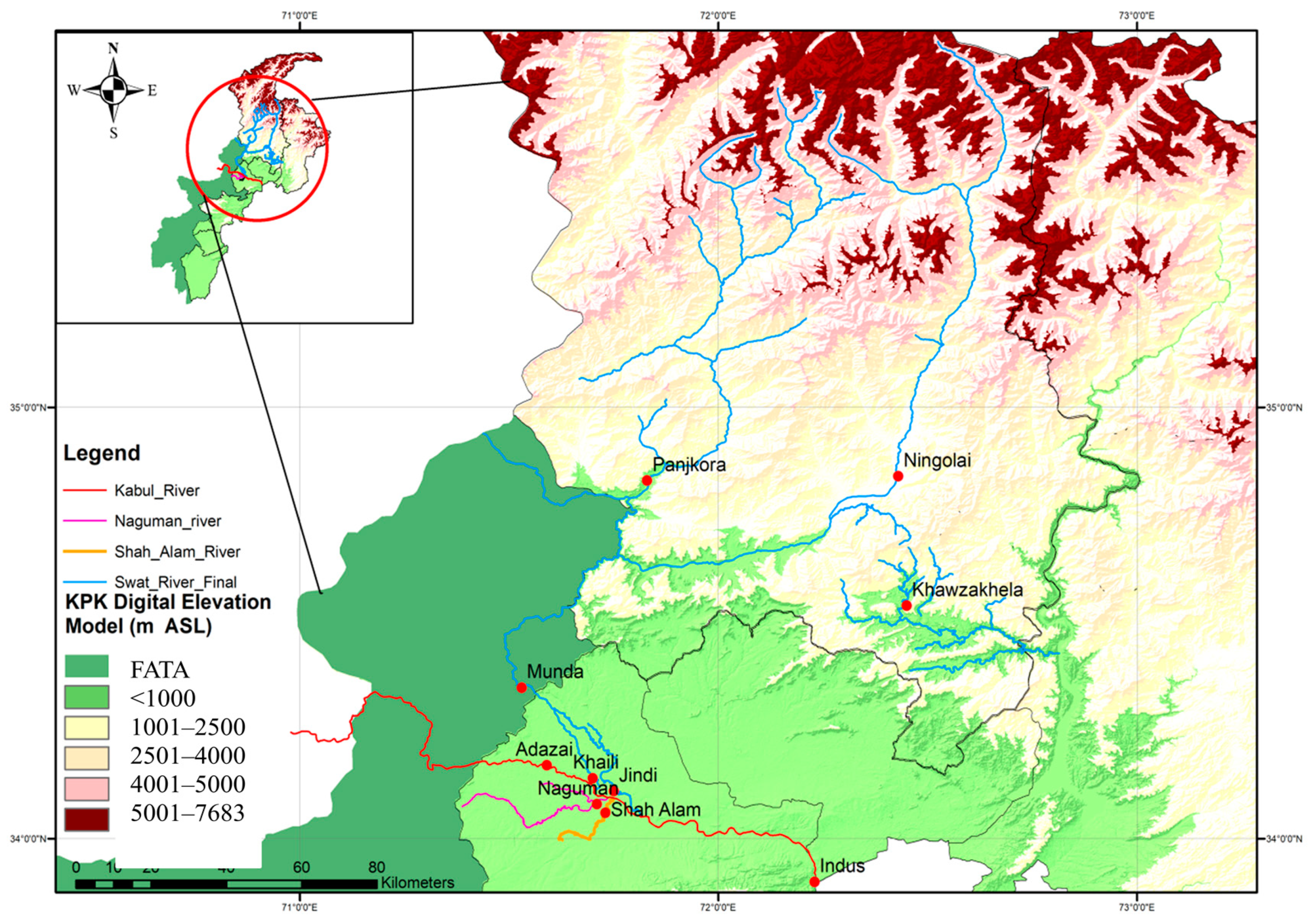
Figure 1 depicts the study area, and its major fragment is Indus basin system in Pakistan. We selected 11 critical locations situated on the Kabul river, Swat river, Indus river, and Jhelum river for FFA. Annual maximum (AM) streamflow data with a record length of more than 30 years is provided by the hydrology and irrigation division, and the summary is illustrated in

Table 1. Summary statistics of annual maximum (AM) flood series record.

Gauging Station	Period	Mean (m3/s)	Cv	Cs	Ck
Attock	1970–2017	13,028	0.29	1.33	4.73
Jindi	1969–2017	300	0.67	1.85	6.81
Munda Headworks	1962–2017	1748	0.73	4.81	31.33
Khwazakhela	1983–2016	1451	0.83	1.56	1.89
Ningolai	1984–2016	242	1.45	2.30	5.61
Khiali	1969–2017	1648	0.82	5.26	34.87
Shah Alam	1987–2017	207	0.71	0.86	−0.13
Naguman	1987–2017	533	0.84	1.74	4.39
Adezai	1987–2017	868	0.67	0.65	−0.44
Timergara	1984–2017	736	0.85	3.09	14.77
Karot	1969–2010	3725	0.67	2.82	9.59

. We noticed that the length of this historical data from eleven gauging stations varies at every station. The Swat river at Munda Headworks has the longest data length of 56 years, while 3 gauging stations at Adezai, Naguman and Shah Alam have 31 years of historical data. Furthermore, all the sites are highly and positively skewed, which implies that the size of the right-tail is larger than the left tail. As shown in Table 1, the value of skewness ranges from 0.65 (Adezai) to 5.26 (Khiali). The variation in the skewness of different sites owes to floods in Monsoon seasons at different times. In the same manner, the kurtosis values are also indexed in Table 1, which presents positive values of kurtosis except for the two sites. This implies that the distribution is heavy-tailed, except for instances where it has acquired negative values.

In addition, we inferred from the unit root stationary test and homogeneity test that the data is stationary and homogeneous for further analysis. It will allow various probability distributions to estimate flood peaks that will not be deviating from the historic trend.

3. Methods

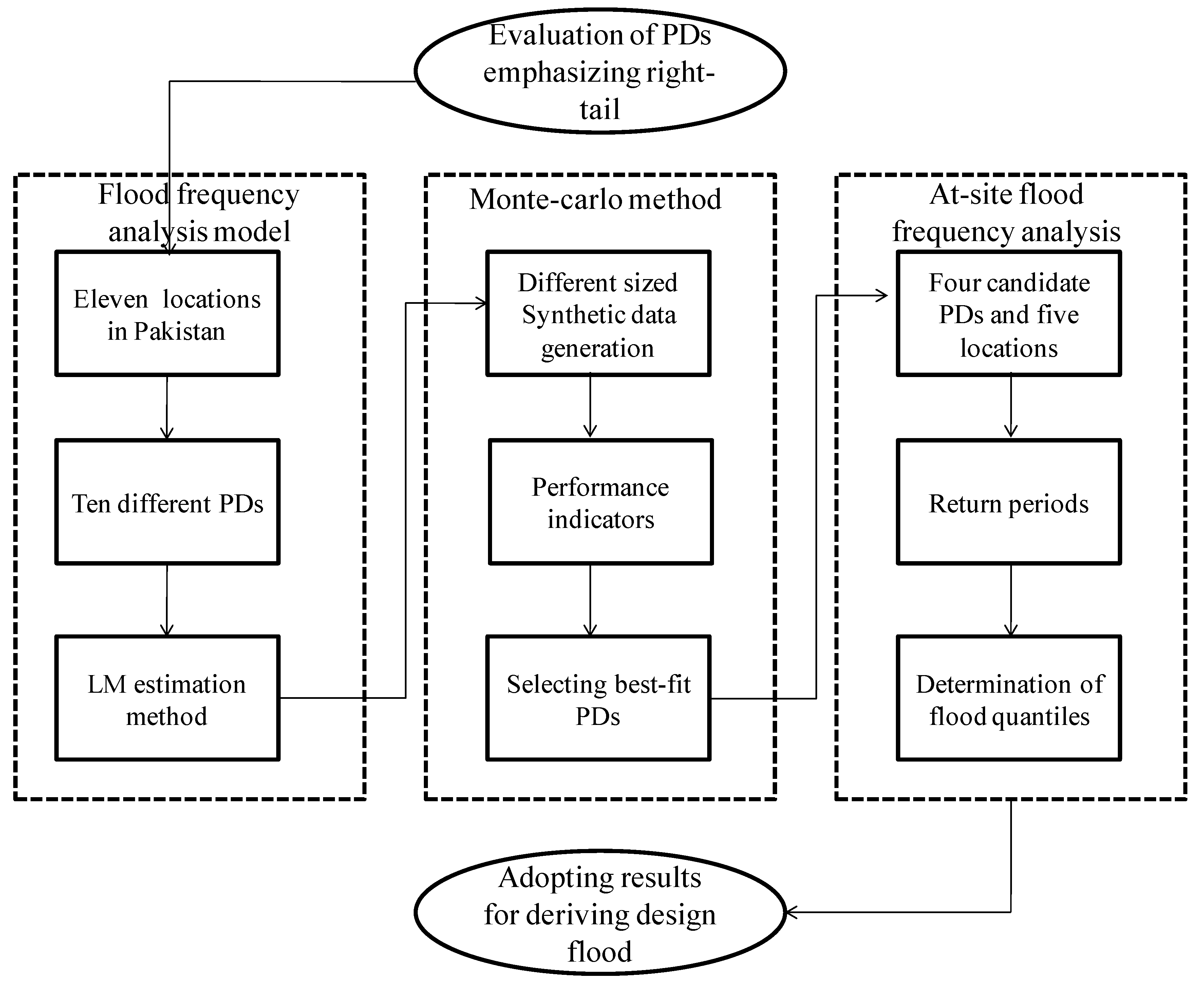
In order to find the best-fit PD for river basins in Pakistan, we employed an AM flood series method. Considering the right-tail events scenario of our study, we followed the procedure in three steps, such as (i) selection of PDs; (ii) selection of parameter estimation method; (iii) carrying out hypothesis test for evaluating goodness-of-fit of PDs to the historical record and applying selection criteria for choice of statistical distribution; (iv) evaluation of the selected PDs with respect to right tail behavior by employing Monte Carlo simulation; and (v) further analyzing the selected PDs with flood frequency curves and estimation of flood quantiles. The flowchart in Figure 2 shows the main procedure for evaluating flood quantiles over Pakistan.

3.1. Probability Distributions

We considered various familiar PDs in this study, namely EXP, GAM, GEV, GLO, GPA, GNO, Gumbel extreme-value type I (GUM), normal (NOR), P3and WEI for carrying out probabilistic modeling of extreme events. Six PDs (GEV, GLO, GNO, GPA, P3 and WEI) have three parameters, and four PDs (EXP, GAM, NOR, and GUM) have two parameters. The probability density functions (PDFs) and parameters of PDs are illustrated in

Table 2. The parameters and probability density functions (PDFs) of contending distributions.

Number	Distribution	Probability Density Function	Parameters
1	EXP	$\mathrm{F}\left(\mathrm{x}\right)=1-\exp \left\{-\left(\mathrm{x}-\mathsf{\xi }\right)/\mathsf{\alpha }\right\}$	$\mathrm{scale}\mathrm{parameter}=\mathsf{\alpha }$ $\mathrm{location}\mathrm{parameter}=\mathsf{\xi }$
2	GAM	$\mathrm{F}\left(\mathrm{x}\right)=\frac{{\mathrm{x}}^{\mathsf{\alpha }-1}\exp \left(\frac{-\mathrm{x}}{\mathsf{\beta }}\right)}{{\mathsf{\beta }}^{\mathsf{\alpha }}\mathsf{\Gamma }\left(\mathsf{\alpha }\right)}$ Γ is the gamma function	$\mathrm{shape}\mathrm{parameter}=\mathsf{\alpha }$ $\mathrm{scale}\mathrm{parameter}=\mathsf{\beta }$
3	GEV	$\mathrm{F}\left(\mathrm{x}\right)=\exp \left\{-\exp \left(-\mathrm{y}\right)\right\}$ $\mathrm{y}={\mathsf{\kappa }}^{-1}\log \left\{1-\mathsf{\kappa }\left(\mathrm{x}-\mathsf{\xi }\right)/\mathsf{\alpha }\right\}$	$\mathrm{shape}\mathrm{parameter}=\mathsf{\kappa }$ $\mathrm{scale}\mathrm{parameter}=\mathsf{\alpha }$ $\mathrm{location}\mathrm{parameter}=\mathsf{\xi }$
4	GLO	$\mathrm{F}\left(\mathrm{x}\right)=\frac{1}{\left\{1+\exp \left(-\mathrm{y}\right)\right\}}$ $\mathrm{y}=-{\mathsf{\kappa }}^{-1}\log \left\{1-\mathrm{k}\left(\mathrm{x}-\mathsf{\xi }\right)/\mathsf{\alpha }\right\}$	$\mathrm{shape}\mathrm{parameter}=\mathsf{\kappa }$ $\mathrm{scale}\mathrm{parameter}=\mathsf{\alpha }$ $\mathrm{location}\mathrm{parameter}=\mathsf{\xi }$
5	GNO	$\mathrm{F}\left(\mathrm{x}\right)=\mathsf{\varphi }\left(\mathrm{y}\right)$ $\mathrm{y}=-{\mathsf{\kappa }}^{-1}\log \left\{1-\mathrm{k}\left(\mathrm{x}-\mathsf{\xi }\right)/\mathsf{\alpha }\right\}$	$\mathrm{shape}\mathrm{parameter}=\mathsf{\kappa }$ $\mathrm{scale}\mathrm{parameter}=\mathsf{\alpha }$ $\mathrm{location}\mathrm{parameter}=\mathsf{\xi }$
6	GPA	$\mathrm{F}\left(\mathrm{x}\right)=1-\exp \left(-\mathrm{y}\right)$ $\mathrm{y}=-{\mathrm{k}}^{-1}\log \left\{1-\frac{\mathsf{\kappa }\left(\mathrm{x}-\mathsf{\xi }\right)}{\mathsf{\alpha }}\right\}$	$\mathrm{shape}\mathrm{parameter}=\mathsf{\kappa }$ $\mathrm{scale}\mathrm{parameter}=\mathsf{\alpha }$ $\mathrm{location}\mathrm{parameter}=\mathsf{\xi }$
7	GUM	$\mathrm{F}\left(\mathrm{x}\right)=\exp \left[-\exp \left\{-\left(\mathrm{x}-\mathsf{\xi }\right)/\mathsf{\alpha }\right\}\right]$	$\mathrm{scale}\mathrm{parameter}=\mathsf{\alpha }$ $\mathrm{location}\mathrm{parameter}=\mathsf{\xi }$
8	NOR	$\mathrm{F}\left(\mathrm{x}\right)=\frac{1}{\mathsf{\sigma }\sqrt{2\mathsf{\pi }}}\exp \left\{-\frac{{\left(\mathrm{x}-\mathsf{\mu }\right)}^2}{\left(2{\mathsf{\sigma }}^2\right)}\right\}$	$\mathrm{scale}\mathrm{parameter}=\mathsf{\sigma }$ $\mathrm{location}\mathrm{paramete}=\mathsf{\mu }$
9	P3	$\mathrm{F}\left(\mathrm{x}\right)=\frac{{\left|\mathrm{x}-\mathsf{\epsilon }\right|}^{\mathsf{\alpha }-1}\exp \left(-\left|\mathrm{x}-\mathsf{\epsilon }\right|/\mathsf{\beta }\right)}{{\mathsf{\beta }}^{\mathsf{\alpha }}\mathsf{\Gamma }\left(\mathsf{\alpha }\right)}$ If $\mathsf{\gamma }\ne 0$, then let $\mathsf{\alpha }=\frac{4}{{\mathsf{\gamma }}^2}$,$\mathsf{\beta }=\frac{1}{2}\mathsf{\sigma }\left|\mathsf{\gamma }\right|$, and $\mathsf{\xi }=\mathsf{\mu }-2\mathsf{\sigma }/\mathsf{\gamma }$	$\mathrm{scale}\mathrm{parameter}=\mathsf{\sigma }$ $\mathrm{shape}\mathrm{parameter}=\mathsf{\gamma }$ $\mathrm{location}\mathrm{parameter}=\mathsf{\mu }$
10	WEI	$\mathrm{F}\left(\mathrm{x}\right)=1-\exp \left[-{\left\{\left(\mathrm{x}-\mathsf{\zeta }\right)/\mathsf{\beta }\right\}}^{\mathsf{\delta }}\right]$	$\mathrm{scale}\mathrm{parameter}=\mathsf{\beta }$ $\mathrm{shape}\mathrm{parameter}=\mathsf{\delta }$ $\mathrm{location}\mathrm{parameter}=\mathsf{\zeta }$

.

3.2. Parameter Estimation Method

Linear moment (LM)method offers small bias, which is an advantage over all other parameter estimation methods [12,33]. Let X₁, X₂, …, X_r be a conceptual random sample of size r, from a continuous function which is quantified by the function ${\mathrm{Q}}_{\mathrm{X}}\left(\mathrm{u}\right)={\mathrm{F}}^{-1}{}_{\mathrm{X}}\left(\mathrm{u}\right)$; let X_1r ≤ X_2r ≤ … ≤ X_rr denote the corresponding ordered statistics. Hosking (1990) defined the r_th L-moment as follows [34]:

$${\mathsf{\lambda }}_{\mathrm{r}}={\mathrm{r}}^{-1}{\displaystyle \sum }_{\mathrm{k}=0}^{\mathrm{r}-1}{\left(-1\right)}^{\mathrm{k}}\left(\begin{array}{c}\mathrm{r}-1\\ \mathrm{k}\end{array}\right)\mathrm{E}\left({\mathrm{X}}_{\mathrm{r}-\mathrm{kr}}\right),$$

(1)

where the order of moment is denoted by r (r = 1, 2 …,) and

$$\mathrm{E}\left({\mathrm{X}}_{\mathrm{tr}}\right)=\frac{\mathrm{r}!}{\left(\mathrm{t}-1\right)!\left(\mathrm{r}-\mathrm{t}\right)!}\underset{0}{\overset{1}{{\displaystyle \int }}}\mathrm{Q}\left(\mathrm{u}\right){\mathrm{u}}^{\mathrm{t}-1}{\left(1-\mathrm{u}\right)}^{\mathrm{r}-\mathrm{t}}\mathrm{du}$$

(2)

L-moment ratios, the L-coefficient of variation (${\mathsf{\tau }}_2$), L-skewness (${\mathsf{\tau }}_3$), and L-kurtosis (${\mathsf{\tau }}_4$) are defined as

$${\mathsf{\tau }}_2=\frac{{\mathsf{\lambda }}_2}{{\mathsf{\lambda }}_1},{\mathsf{\tau }}_3=\frac{{\mathsf{\lambda }}_3}{{\mathsf{\lambda }}_2},{\mathsf{\tau }}_4=\frac{{\mathsf{\lambda }}_4}{{\mathsf{\lambda }}_2}$$

(3)

3.3. The Goodness-of-Fit and Selection Criteria

The Kolmogorov-Smirnov (KS) is a goodness-of-fit statistics which is used to decide if a sample comes from a population with a specific distribution [33]. At the selected level of significance, the p-value is scrutinized for testing the hypothesis. The KS test is defined by the following equation:

$$\mathrm{D}=\underset{1\le \mathrm{i}\le \mathrm{n}}{\max }\left[\mathrm{F}\left({\mathrm{X}}_{\mathrm{i}}\right)-\frac{\mathrm{i}-1}{\mathrm{n}},\frac{\mathrm{i}}{\mathrm{n}}-\mathrm{F}\left({\mathrm{X}}_{\mathrm{i}}\right)\right],$$

(4)

where sample size is denoted by n, and the cumulative distribution function is expressed by $\mathrm{F}\left({\mathrm{X}}_{\mathrm{i}}\right)$.

We conducted the KS test for 11 locations shown in

Table 3. Computed p-values of contending distributions for the selected locations.

Gauging Stations	EXP	GUM	GPA	GNO	GLO	GEV	GAM	P3	WEI	NOR
Attock	0.032	0.015	0.048	0.015	0.015	0.031	0.016	0.015	0.032	0.038
Jindi	0.046	0.004	0.034	0.010	0.009	0.014	0.024	0.032	0.016	0.019
Munda Headworks	0.038	0.085	0.038	0.027	0.022	0.025	0.965	0.049	0.051	0.989
Khwazakhela	0.014	0.051	0.002	0.002	0.014	0.014	0.014	0.002	0.001	0.061
Ningolai	0.071	0.049	0.035	0.035	0.035	0.035	0.035	0.070	0.015	0.075
Khiali	0.072	0.072	0.041	0.045	0.042	0.049	0.045	0.045	0.046	0.037
Shah Alamriver	0.018	0.073	0.018	0.039	0.071	0.050	0.018	0.018	0.018	0.054
Naguman	0.002	0.018	0.002	0.002	0.002	0.002	0.002	0.002	0.002	0.051
Adezai	0.080	0.039	0.018	0.018	0.039	0.039	0.018	0.018	0.018	0.052
Timergara	0.013	0.014	0.053	0.014	0.014	0.019	0.016	0.016	0.014	0.061
Karot	0.029	0.051	0.029	0.007	0.0009	0.0009	0.050	0.050	0.041	0.082

to determine whether the data obeys the distribution. We computed the p-values for each distribution to provide a testimony of fitness of PDs for obeying the empirical data. When the p-value is greater than 0.05, it implies that the data does not obey the distribution at 5% significance level [34,35].

An appropriate PD must be selected by making use of the statistical criteria [18]. In this regard, the PDs are evaluated by two criterions, the Akaike information criteria (AIC) and the root mean square error (RMSE). AIC refers to an information-based criterion which encourages the selection of PDs under definite conditions [35,36]. We employed RMSE, which is another criterion offering selection in this study, and is commonly directed for measuring the fit of the PDs to the available record. We persisted with these criterions to measure the descriptive strength of PD_S. These are defined by the following Equations [33,37]:

$$\mathrm{RMSE}=\sqrt[]{\frac{{{\displaystyle \sum }}_{\mathrm{i}=0}^{\mathrm{n}}\left(\mathrm{P}\left(\mathrm{i}\right)-\mathrm{P}\left(\mathrm{i}\right)\right){}^2}{\mathrm{n}}},$$

(5)

$$\mathrm{AIC}=\left[\ln \left[\frac{1}{\mathrm{n}}{\displaystyle \sum }_{\mathrm{i}=0}^{\mathrm{n}}\left({\mathrm{P}}_{\mathrm{the}\left(\mathrm{i}\right)}-{\mathrm{P}}_{\mathrm{emp}\left(\mathrm{i}\right)}\right){}^2\right]\right]+2\mathrm{K}$$

(6)

where n is the size of the sample, K is the number of parameters of the distribution, P_the is the theoretical probability of the distribution, and P_emp is empirical probability measured by the Gringorten plotting position formula [38]:

$${\mathrm{P}}_{\mathrm{emp}\left(\mathrm{i}\right)=\frac{\mathrm{i}-0.44}{\mathrm{n}+0.12}}.$$

(7)

The comparative performances of PD are measured by AIC, while RMSE measures the fitting of candidate distribution to the AM series of a gauging station. We used Equations (5) and (6) to compute the values of AIC and RMSE corresponding to each PD. The lower AIC and RMSE values, as illustrated in

Table 4. Calculated values of Akaike information criteria (AIC) and root mean square error (RMSE) of probability distributions for different locations.

Distributions	Criteria	Attock	Jindi	Adezai	Naguman	Timergara	Khiali	Khwazakhela	Munda	Ningolai	Shah Alam	Karot
NOR	RMSE	0.0457	0.0566	0.0823	0.0989	0.0854	0.1187	0.1385	0.1177	0.179	0.986	0.1471
	AIC	−290.16	−275.33	−148.77	−137.43	−161.29	−202.77	−128.39	−223.58	−107.52	137.61	−161.13
WEI	RMSE	0.0404	0.0404	0.0601	0.0319	0.0494	0.092	0.0393	0.0671	0.0732	0.056	0.0755
	AIC	−301.98	−308.33	−168.28	−207.58	−198.4	−227.73	−214	−296.47	−166.47	−172.7	−201.55
P3	RMSE	0.0385	0.0394	0.0644	0.0318	0.0486	0.0909	0.0407	0.068	0.1045	0.0584	0.0893
	AIC	−306.65	−310.77	−163.97	−207.7	−199.51	−228.98	−211.55	−294.99	−143.01	−170.1	−192.08
GAM	RMSE	0.0385	0.0422	0.062	0.0357	0.0487	0.0921	0.0792	0.082	0.0741	0.0606	0.1053
	AIC	−306.48	−304.15	−166.3	−200.46	−199.49	−227.65	−166.38	−274.04	−165.69	−167.76	−178.55
GEV	RMSE	0.0387	0.0392	0.0712	0.0301	0.0477	0.0813	0.0489	0.0472	0.0587	0.0711	0.0446
	AIC	−306.18	−311.37	−157.74	−211.13	−200.81	−239.85	−199.15	−335.73	−181.03	−157.87	−248.84
GLO	RMSE	0.0374	0.0393	0.0804	0.0337	0.0486	0.0759	0.0535	0.0424	0.0596	0.0801	0.0414
	AIC	−309.45	−310.95	−150.27	−204.02	−199.63	−246.59	−193.08	−347.81	−180.07	−150.5	−255.08
GNO	RMSE	0.0382	0.039	0.0689	0.0281	0.0474	0.0848	0.0414	0.054	0.0572	0.0663	0.0603
	AIC	−307.44	−311.77	−159.79	−215.33	−201.24	−235.72	−210.45	−320.7	−182.75	−162.18	−224.25
GPA	RMSE	0.0569	0.0486	0.0511	0.032	0.0514	0.0949	0.0408	0.0655	0.0566	0.0512	0.0655
	AIC	−269.03	−290.11	−178.26	−207.37	−195.22	−224.73	−211.39	−299.16	−183.42	−178.26	−217.39
GUM	RMSE	0.0417	0.0391	0.0711	0.0597	0.0556	0.0888	0.1018	0.0783	0.1425	0.0772	0.1049
	AIC	−298.95	−311.44	−157.9	−168.67	−190.48	−231.25	−149.33	−279.22	−122.58	−152.78	−178.84
EXP	RMSE	0.0786	0.066	0.064	0.0317	0.053	0.096	0.0638	0.67	0.104	0.0515	0.0779
	AIC	−238.13	−260.41	−163.87	−207.96	−193.66	−223.64	−181.12	−296.73	−143.07	−177.89	−203.25

, indicates a better distribution so the best-fit PD will have the minimum value of AIC and RMSE.

3.4. Monte Carlo Simulation

The goodness-of-fit indicates the goodness within the reach of available record; therefore, it is unable to indicate the performance of PDs at the right-tail segment. The performance of PDs regarding right-tail events is significant for the design of critical hydraulic structures for selection of design flood against a small exceedance probability [27]. Moreover, to reduce the lifetime risk of hydraulic structures, the flood quantile with a very small exceedance probability has to be chosen. Therefore, in order to develop the convincing idea of the behavior of contending PD at the extreme tail, we probed PD by carrying out the Monte Carlo simulation. Accordingly, a base distribution should be chosen other than the contending distributions. Cunnane (1989) proposed the five-parameter Wakeby distribution as a parent distribution for its versatility [8]. Considering its credibility, we adopted it as a base distribution for the generation of long synthetic data series to examine the performance of PDs corresponding to rare events.

We employed a historical record of four major rivers to obtain parameters of parent distribution, and later estimated random number samples of different sizes n (n = 20, 50, 100). The parameters of the Wakeby distribution are summarized in

Table 5. Parameters values of Wakeby distribution for five stations in Pakistan.

Parameter	ξ	α	β	ϒ	δ
Panjkora river	130.97	677.34	0.12	0.00	0.00
Khiali	293.02	4122.62	2.87	52.32	0.82
Shah Alamriver	30.11	206.28	0.164	0.00	0.00
Ningolai	0.83	0.00	0.00	135.22	0.44
Adezai	97.43	1032.69	0.34	0.00	0.00

. Houghton (1978) defined the inverse function of Wakeby distribution as follows [39]:

$$x\left(\mathrm{F}\right)=\mathsf{\xi }+\frac{\mathsf{\alpha }}{\mathsf{\beta }}\left(1-{\left(1-\mathrm{F}\right)}^{\mathsf{\beta }}\right)-\frac{\mathsf{\gamma }}{\mathsf{\delta }}\left(1-{\left(1-\mathrm{F}\right)}^{-\mathsf{\delta }}\right).$$

(8)

We obtained parameters of base distribution from the observed data and generated the random samples of different lengths n (n = 20, 50, 100). Next, we calculated flood quantiles of contending distributions from the random samples against a higher return periods T (T = 100, 200). The higher return periods of 100 and 200 years induce right-tail for each PD, so the simulation setup was repeated 1000 times to obtain flood quantiles at the extreme tail for different random samples. Similarly, to quantify the degree of prediction of extreme events, the composition proceeded for the selected four rivers for each of the candidate distributions. Later, we employed three performance indexes, namely, relative bias (RB), absolute relative bias (ARB), and relative root mean square error (RRMSE), for the flood quantiles secured by PDs at the extreme events. These are defined by the following equations [40,41]:

$$\mathrm{RB}=\frac{1}{\mathrm{S}}{\displaystyle \sum }_{\mathrm{i}=1}^{\mathrm{S}}\left(\frac{{\left({\hat{\mathrm{Q}}}_{\mathrm{T}}\right)}_{\mathrm{i}}-{\mathrm{Q}}_{\mathrm{T}}}{{\mathrm{Q}}_{\mathrm{T}}}\right){}^2,$$

(9)

$$\mathrm{ARB}=\frac{1}{\mathrm{S}}{\displaystyle \sum }_{\mathrm{i}=1}^{\mathrm{s}}\left|\frac{{\left({\hat{\mathrm{Q}}}_{\mathrm{T}}\right)}_{\mathrm{i}}-{\mathrm{Q}}_{\mathrm{T}}}{{\mathrm{Q}}_{\mathrm{T}}}\right|,$$

(10)

$$\mathrm{RRMSE}=\sqrt{\frac{1}{\mathrm{S}-1}{\displaystyle \sum }_{\mathrm{i}=0}^{\mathrm{n}}\left(\frac{\left({\hat{\mathrm{Q}}}_{\mathrm{T}}\right)-{\mathrm{Q}}_{\mathrm{T}}}{{\mathrm{Q}}_{\mathrm{T}}}\right){}^2,}$$

(11)

where Q_T is given parent quantile, ${\left({\hat{\mathrm{Q}}}_{\mathrm{T}}\right)}_1$…${\left({\hat{\mathrm{Q}}}_{\mathrm{T}}\right)}_{\mathrm{s}}$ are estimators for the samples generated by parent distribution, and S is the number of Monte Carlo trials.

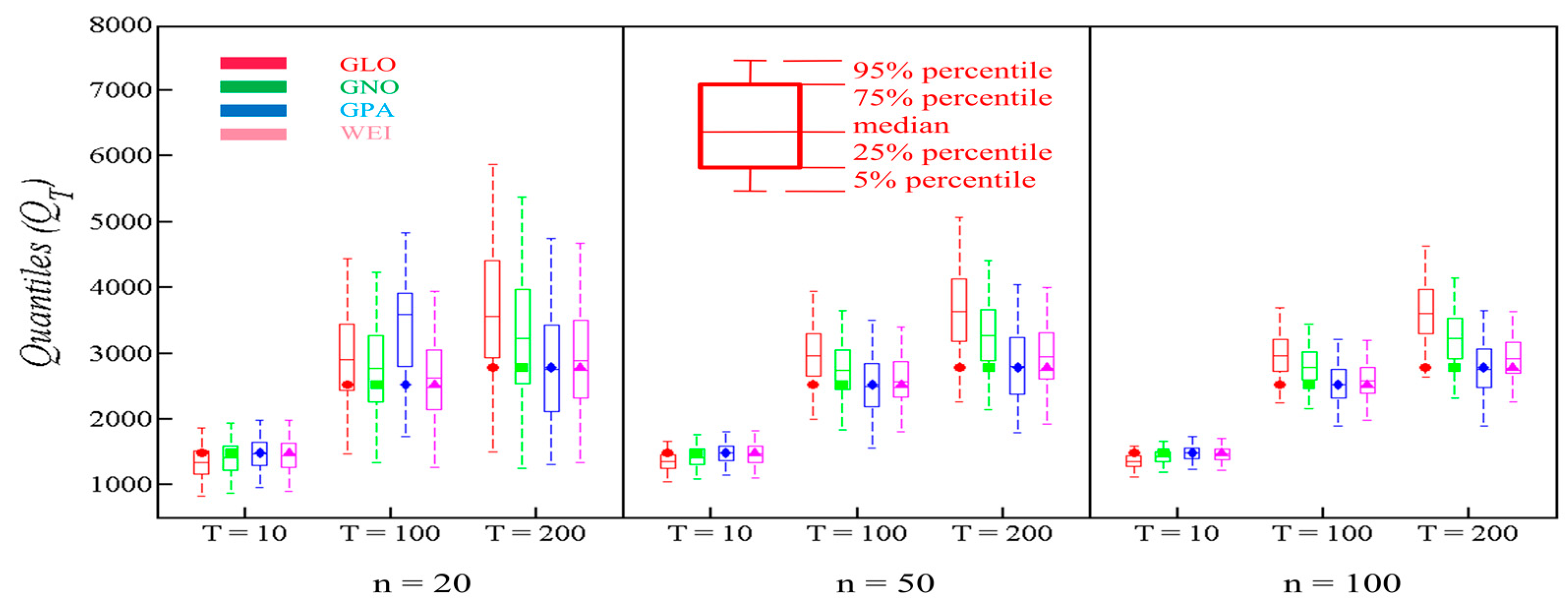
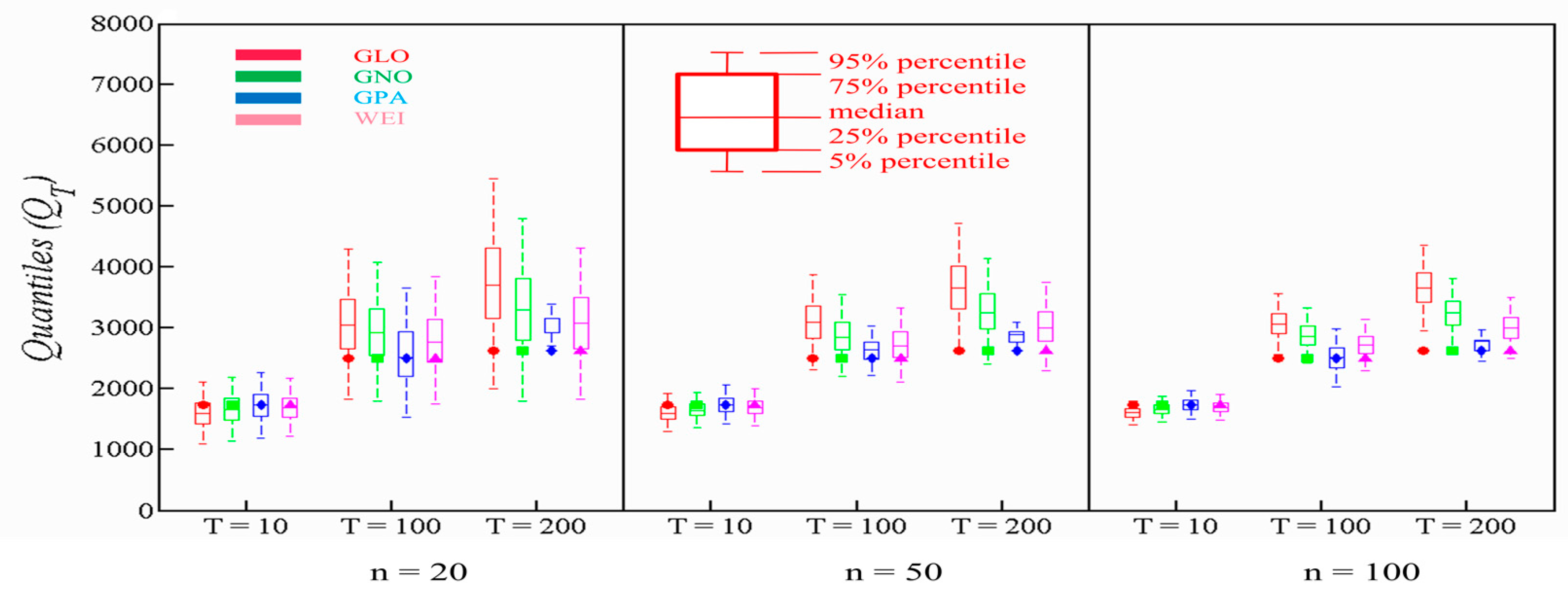
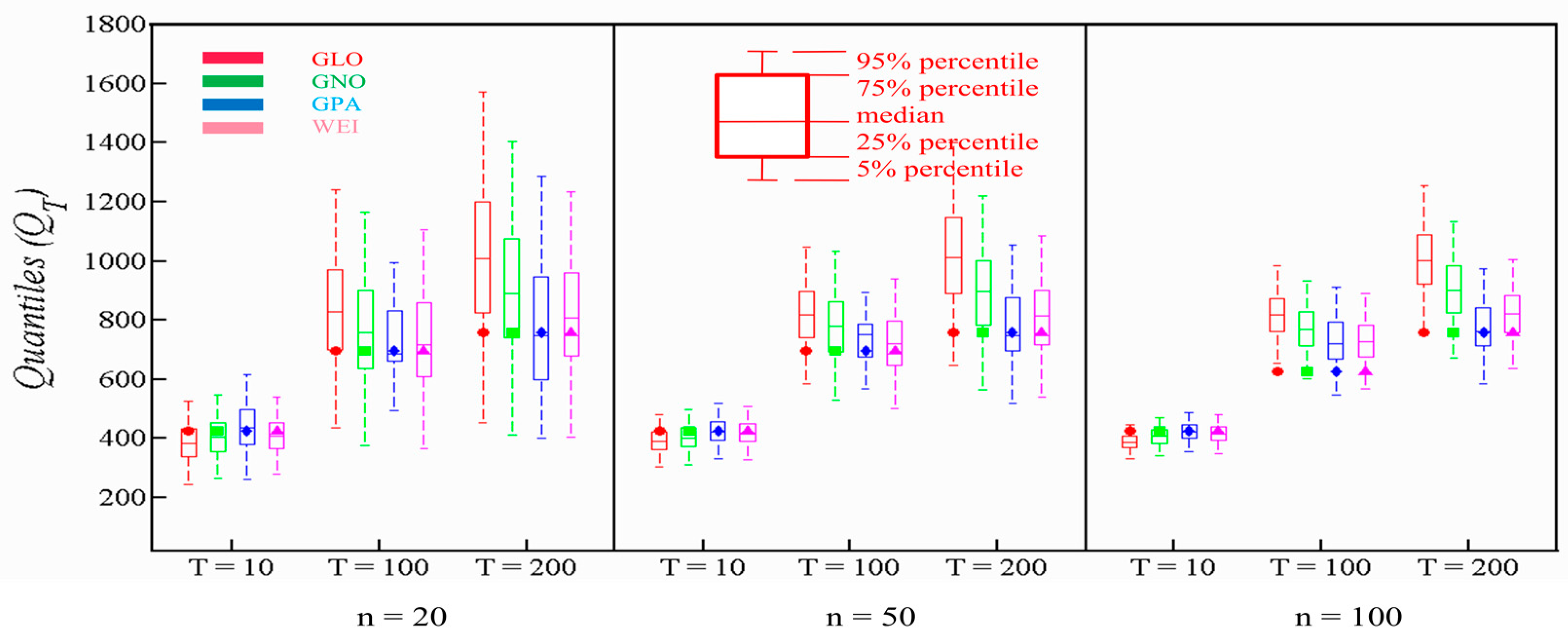
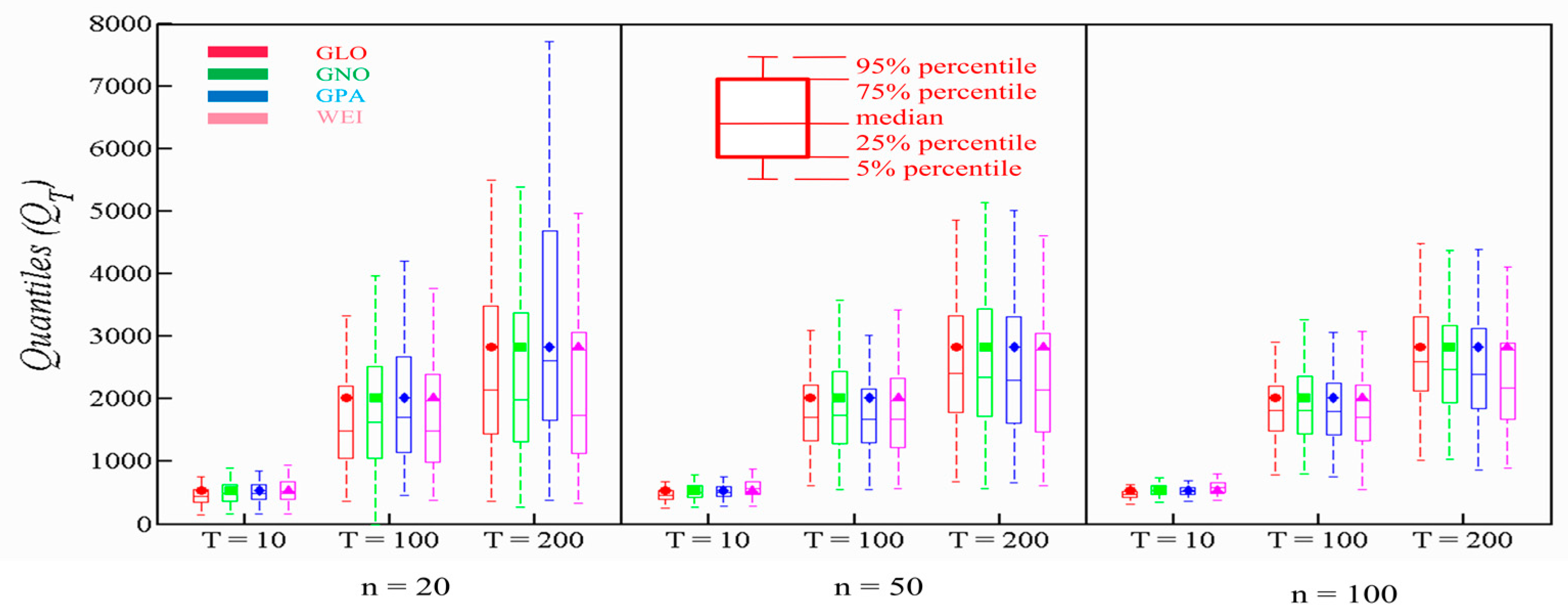
The lower RB, ARB and RRMSE values endorse the most reliable distribution. We used Equations (9)–(11) to compute the values of RB, ARB, and RRMSE. We considered the flood quantiles having return periods of 100 and 200 years, to probe the PDs at the right-tail. Additionally, we engaged boxplots with quantiles estimates for higher return periods of T = 100 and T = 200, and a small return period of T = 10. Boxplots for each contending PD at every station was plotted to assess their performance. We analyzed narrowness of 90% percentile of boxplots and parent quantiles to evaluate the performance of PDs. The 90% confidence interval is represented by each boxplot in each case. The 50% interquartile range is represented by the box with 75% and 25% as upper and lower bounds. Moreover, the upper and lower bounds of whiskers represent 95% and 5% percentile.

4. Results

4.1. The Goodness-of-Fit and Selection of PDs

The p-value manifested in Table 3 indicates the fitting of sample data to a particular distribution at 5% significance level. To this extent, the p-values lower than 0.05 indicates that the historical record of the AM series belongs to the particular distribution [18]. It can be inferred from the results illustrated in Table 5 that NOR distribution is not in consonance with the historical record of six locations at 5% significance level. Next, the GUM distribution does not obey the available record of Munda Headworks, Khwazakhela, Karot, Khiali and Shah Alam. In addition to that, EXP distribution does not follow the empirical data of Ningolai, Khialiand Adezai, with higher p-value. Meanwhile, P3, GAM and GLO failed to follow AM series at one location each. For other locations, the assumption that the historical data belongs to the candidate distribution cannot be rejected at the 5% significance level.

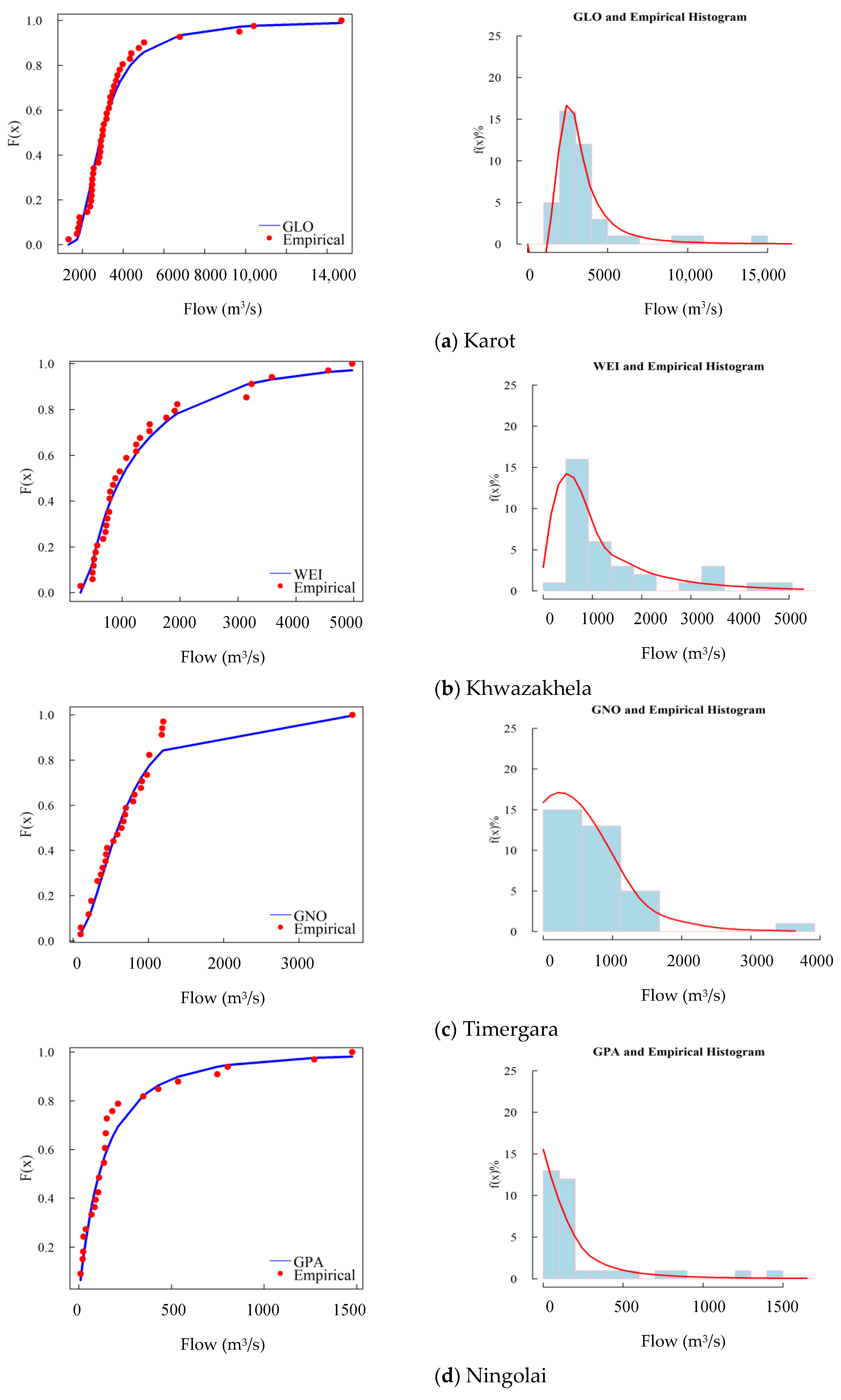
Later, we employed RMSE and AIC to compare the results of contending distributions as manifested in Table 4. We computed values of RMSE and AIC for each PD at all stations. RMSE and AIC values for GLO are smallest at Attock, Khiali and Munda Headworks. Moreover, GNO adhered to the lowest values for Jindi, Naguman and Panjkora. GPA and WEI fit the AM peak flow series of Adezai and Khwazakhela, respectively possessing lowest RMSE and AIC values at these gauging stations. It can be inferred from the above that different PDs fits the historical AM flood series of different gauging stations. As indicated in Table 4, GLO persisted with better performance at four locations, while GNO and GPA advanced with smaller magnitudes of goodness criteria on three locations each. WEI was chosen as the best distribution for Khwazakhela gauging station. Table 4 demonstrates the fitted PDs corresponding to each location in the Indus basin system in Pakistan. The plot in Figure 3a–d illustrates the fitted distributions for observed data at Karot, Khwazakhela, Timergara and Ningolai. Figure 3 yields the fitted distributions to the empirical frequencies of the respective stations. The empirical frequencies are shown by lines, while the points represent the fitted distribution. The plots demonstrated that GLO, WEI, GNO and GPA are the best-fit for the AM series of the respective gauging stations. It can be inferred from the empirical histogram plotted in Figure 2a–d that the distributions that describe the datasets of the respective gauging stations also represent the AM flood series very well. The PDFs of the distributions are plotted to fit the empirical histograms of available records. GLO generally fit the data series with very high skewness, while GPA fit with moderate skewness, except for Ningolai. WEI and GNO also fit the AM flood series with high skewness.

4.2. Performance at Right-Tail of PDs

We engaged Wakeby distribution for generation of synthetic data series of different sizes n (n = 20, 50, 100) from the historical data series of Indus basin system of Pakistan to assess the quantile estimates of four PDs with return periods T (T = 100 and 200). The computed values of RB, ARB, and RRMSE are illustrated in

Table 6. Calculated relative bias (RB), absolute relative bias (ARB) and relative root mean square error (RRMSE) values for different probability distributions.

Title	Sample Size	Return Period	GLO			GNO			GPA			WEI
			RB	ARB	RRMSE	RB	ARB	RRMSE	RB	ARB	RRMSE	RB	ARB	RRMSE
Panjkora	n = 20	T = 100	18.24	27.07	35.31	11.75	24.30	31.43	33.38	36.73	42.78	4.46	21.05	26.52
		T = 200	33.69	40.16	52.11	18.36	31.63	41.03	3.90	28.14	36.20	7.17	25.08	32.30
	n = 50	T = 100	17.76	20.98	25.82	9.57	16.10	20.55	1.18	14.93	18.84	3.61	13.23	17.03
		T = 200	31.92	33.43	40.26	18.65	22.72	28.38	3.59	16.88	21.70	7.09	15.53	19.85
	n = 100	T = 100	17.58	18.69	22.31	11.16	13.61	16.74	1.36	10.03	12.68	2.95	9.56	12.31
		T = 200	30.72	31.03	35.18	16.79	18.58	23.18	0.43	12.37	15.47	5.69	10.92	14.08
Adezai	n = 20	T = 100	22.74	27.00	33.19	17.47	22.80	28.46	5.09	15.21	19.55	11.69	18.31	23.19
		T = 200	42.36	43.84	52.62	25.90	30.09	37.36	16.44	17.59	23.54	17.91	22.70	28.57
	n = 50	T = 100	24.13	24.78	28.56	14.83	16.47	19.82	6.19	8.70	11.49	9.03	12.25	15.19
		T = 200	39.41	39.59	44.00	24.22	25.02	29.22	9.63	10.76	13.28	15.16	16.81	20.74
	n = 100	T = 100	22.67	22.72	24.76	14.89	15.25	17.44	0.47	7.53	9.33	9.03	10.43	12.54
		T = 200	38.87	38.88	41.09	23.49	23.55	25.98	4.69	6.58	8.70	14.02	14.49	16.82
Shah Alam	n = 20	T = 100	21.21	27.75	35.79	12.13	23.50	30.79	7.55	16.54	23.97	6.29	20.94	26.77
		T = 200	35.70	40.98	52.12	21.77	30.43	40.00	6.09	26.19	34.67	9.85	22.94	30.35
	n = 50	T = 100	18.41	20.67	25.47	12.23	17.14	21.39	6.43	11.99	15.54	4.30	12.63	15.94
		T = 200	34.92	35.68	42.24	18.94	22.13	28.02	3.87	14.57	19.21	7.62	15.26	19.26
	n = 100	T = 100	17.98	18.45	21.62	10.92	12.89	16.00	4.12	9.32	11.52	4.91	9.80	12.26
		T = 200	32.74	32.87	36.43	19.28	20.38	24.31	2.62	9.81	12.86	8.00	11.40	14.10
Ningolai	n = 20	T = 100	−8.75	44.99	58.65	3.37	53.79	84.19	−1.14	42.05	55.51	5.13	60.97	117.79
		T = 200	−2.94	51.54	70.27	−1.16	58.74	97.14	14.45	55.43	77.57	−8.95	60.81	92.93
	n = 50	T = 100	−7.46	30.21	37.94	1.41	40.17	62.79	−7.45	32.66	43.03	0.83	43.18	79.70
		T = 200	−3.60	36.65	49.91	1.80	45.10	70.49	−3.33	42.80	57.98	−4.84	47.76	79.09
	n = 100	T = 100	−4.49	24.39	31.87	−0.24	29.81	41.78	−4.43	26.49	34.33	−2.26	34.32	58.51
		T = 200	1.18	28.16	39.73	−0.17	35.33	61.11	−5.77	32.47	43.63	−9.64	37.68	63.03

. The smallness in the magnitude of RB, ARB, and RRMSE indicates better performance of the candidate distribution. Moreover, we also used the boxplots to determine the goodness of prediction.

For Panjkora, the RB of GLO is high, and its performance descends when the return period is increased for all sample sizes. By contrast, GPA performed better than other contending distributions, with respect to RB, especially with the growth of the return period for all sample sizes. In terms of ARB and RRMSE, WEI and GPA perform better for all return periods and sample sizes, particularly, GPA behaved well for all sample sizes. To this extent, the robustness of GPA is observed, which is closely followed by WEI. From Figure 4, it can be concluded that GPA and WEI maintained narrowest 90% confidence interval for right-tail events, and the parent quantile is also observed within a 50% interquartile range. GLO and GNO failed to maintain the narrowest 90% confidence interval, although the true population was observed within a 90% confidence interval. The results for a smaller return period of T=10 are comparable, however, GPA and WEI performed slightly better here as well.

For Adezai, again, the RB of GLO endured higher magnitudes among all PDs at the right-tail portion for all sample sizes. The performance of GPA is significant in contrast to other PDs in terms of RB with high return periods T = 100 and200 for all sample sizes. The performance of GPA is significant when evaluated in terms of ARB and RRMSE, while the performances of GNO and GLO are poor. WEI also advanced with better performance in contrast to an inferior showing of GNO. Figure 5 exhibits the robustness of GPA when compared to other available options, especially GNO and GLO. The true population is not falling within the 90% confidence interval for GLO, particularly for larger sample sizes in contrast to other available options. Additionally, GPA observed the narrowest 90% confidence interval for right-tail events. WEI also performed better particularly when compared to GLO and GNO.

For Shah Alam river, the trend of poor performance of GLO continued as the performance indicator shows a downward trend. GPA behaved much better in terms of RB when the return period increased, regardless of sample size. Again, GPA adhered to smaller values of ARB and RRMSE for different sample sizes and return periods, which is closely followed by the WEI distribution. The values of ARB and RRMSE are considerably smaller for GNO with a larger sample size of 100. In this way, the behavior of GPA is superior to other distributions when evaluated in terms of these indicators. According to Figure 6, the narrowest confidence interval of 90% is observed by WEI, which is followed by GPA. Additionally, the parent quantile for GPA and WEI is also falling within the 50% interquartile range except for a single instance for both GPA and WEI. Furthermore, GLO performed poorly by failing to contain the true population within a 90% confidence interval for large sample size. Hence, the behavior of GLO and GNO is quite poor.

Whereas for Ningolai, GLO performed substantially well in terms of RB, whereby the lowest RB was observed for all sample sizes by GLO. RB value of WEI was observed as lowest for T = 200 for larger sample sizes. Additionally, in terms of ARB and RRMSE, the behavior of GLO is superior to other distributions, whereas GPA observed lower ARB and RRMSE values. Moreover, GPA also persisted with good performance by obtaining lower values of RB, ARB and RRMSE. Figure 7 illustrates that all the contending distributions contained the true population within the 50% interquartile range, and the boxplots for smaller return periods are comparable. However, for right-tail events, WEI exhibited the smallest 90% confidence interval for all sample sizes. GPA also performed better, except for a single event of smaller sample size. On the other hand, GNO and GLO performed quite poorly in this case. From these observations, it can be inferred that GPA and Weibull persistently performed better than other distributions, whereas the performance of GNO and GLO is poor for all cases. Hence, GPA and WEI predicted rare floods of 100 years and 200 years, better than the other contending distributions and these can be trusted by engaging in FFA of selected rivers in Pakistan.

4.3. Comparison of Flood Quantiles

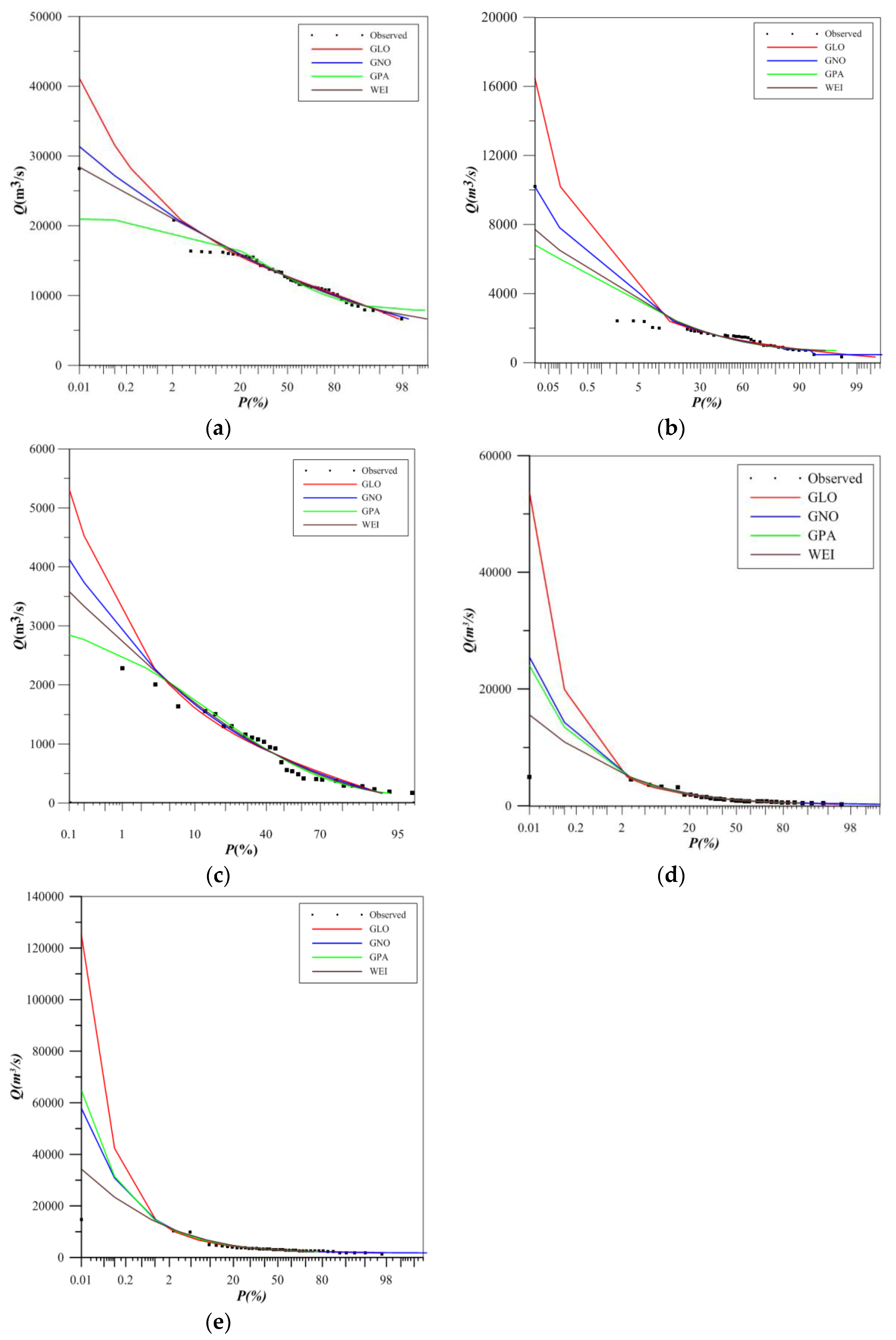
To address any uncertainty, we carried out at-site frequency analysis for the available record of five locations within the Indus basin of Pakistan for adopting the best-fit distribution. The magnitudes of flood quantiles corresponding to return period are illustrated in

Table 7. Flood quantiles estimated by different PDs in Pakistan.

Location	Distribution	Return Period
		20	50	80	100	200
Attock	GLO	19,284	21,813	23,177	23,843	25,995
	GNO	19,322	21,324	22,298	22,750	24,122
	GPA	19,128	19,163	20,232	20,333	20,568
	WEI	19,284	21,042	21,858	22,229	23,322
Khiali	GLO	3306	4337	4975	5308	6490
	GNO	3402	4289	4776	5016	5794
	GPA	3447	4142	4475	4628	5081
	WEI	3431	4181	4558	4735	5280
Adezai	GLO	1995	2570	2904	3073	3646
	GNO	2028	2503	2748	2866	3235
	GPA	2037	2331	2425	2500	2633
	WEI	2031	2435	2630	2720	2991
Karot	GLO	7567	11,071	13,545	14,926	20,287
	GNO	8156	11,579	13,711	15,823	18,721
	GPA	8099	11,401	13,480	14,575	18,479
	WEI	8484	11,490	13,160	13,980	16,638
Khwazakhela	GLO	3647	5462	6701	7381	9956
	GNO	3915	5619	6645	7171	8979
	GPA	3934	5542	6491	6975	8627
	WEI	4050	5521	6314	6700	7928

. The quantiles estimated by different PDs against smaller return periods are comparable to each other. However, the difference in magnitude is sizeable for higher return periods. In this case, GLO has the largest quantiles against a higher return period of 200 years, whereas the lower return periods almost induce similar magnitudes of the hydrological variable. Figure 8a–e demonstrates the flood frequency plots of empirical and estimated flood quantiles of the four distributions. From the flood frequency curves, it can be concluded that higher estimates of quantiles are consummated by GLO and GNO, but the frequency curves for Karot, Khwazakhela and Attock are linear for WEI. Furthermore, frequency curves at Khiali and Adezai are linear for GPA. Considering the frequency curves, it can be inferred that GPA and WEI are unfolded as more viable options for estimation of flood quantiles.

5. Discussions

This study gives us a convincing lead after probing PDs with more consideration being given to the right-tail quantiles to minimize risk to important hydraulic structures in Pakistan. We used the KS method to evaluate the fitting of PDs to the historical data of the selected stations. From our results, the goodness-of-fit of NOR distribution could not concede to six stations. In addition, we observed that GUM could not follow the empirical data of Shah Alam, Munda Headworks, Khwazakhela, Karot and Khiali, while the rest of the PDs fit to the historical data series, except for a few instances. The performance indicators for evaluating descriptive ability were applied for selection of PDs for various locations. In this case, the AIC and RMSE values of all the PDs were estimated, and divergent results were received in return. GLO advanced with the lowest AIC and RMSE values for four stations, while GPA and GNO were found fitting the AM series of three stations each. Additionally, WEI fitted the historical data series of Khwazakhela. The Cumulative Distribution Function (CDF) plots for GLO, GNO, GPA and WEI indicate the fitting of theoretical frequencies of these distributions to the empirical frequencies of respective gauging stations. The CDF plots of PDs supported the results presented by goodness-of-fit test by fitting to the empirical frequencies.

The empirical histograms are also plotted for GLO, GNO, GPA and WEI against the respective fitted observed data. The empirical histograms indicated the fitting of these distributions to the observed data. Next, we evaluated four PDs, namely GLO, GNO, GPA and WEI, for their predictive behaviors by using Monte Carlo (MC) simulations. The results of the Monte Carlo simulation were assessed through performance indicators, such as RB, ARB and RRMSE. The PDs were also evaluated with the help of boxplots. As a result, we identified GPA and WEI as the best choice for estimating right-tail quantiles in all cases.

The flood quantiles for different return periods were estimated by GLO, GNO, GPA and WEI for five stations. The largest flood quantiles are exhibited by GLO for higher return periods, whereas, for lower return periods, the flood quantiles estimated by all distributions are almost identical. The plots for flood frequency curves were developed for the observed and estimated flood quantiles of contending distributions. The curves demonstrate the linearity of frequency curves of GPA and WEI for the selected five locations. Since our study focuses on proposing PDs for Pakistan to counter the menace of flash floods, therefore, the performance against higher return periods is highly endorsed. Different PDs have been identified by researchers in Pakistan during the last decade employing goodness-of-fit tests. Zamir (2009) identified GNO as the best-fit PD followed by GPA from estimated flood quantiles and regional growth curve using the Monte Carlo method [42]. Batool (2017) carried out FFA on 17 locations of Chenab, Ravi, Sutlej, Indus, and Jhelum river, and found that GPA suits most of the locations after applying the goodness-of-fit test [43]. Zakaullah (2012) advocated GUM distribution after carrying out FFA of Jhelum river in Pakistan by applying chi-square test [44]. Ishfaq (2015) recommended GPA by conducting at-site flood frequency analysis using L-moments, TL-moments, and maximum likelihood estimation, using annual maximum stream flows in Pakistan after employing goodness-of-fit tests [45]. Another study carried out by Ishfaq (2015) suggested the use of GPA for different locations in Pakistan using annual maximum rainfall data, by adopting L-moments and TL-moments [46].

The PDs identified in these studies are obtained usually by the goodness-of-fit tests. Therefore, we performed a Monte Carlo simulation to thoroughly analyze the performance of PDs at the right-tail section, followed by estimation of flood quantile against return periods for several locations in Pakistan. Overall, even though a few studies used GNO or GUM distribution functions to characterize the dynamics of the flood, most previous studies are still consistent with our finding that the GPA usually performs best over Pakistan. The classical goodness-of-fit test in this study also unveiled GNO and GLO as the most reliable PD for a few locations, but they consistently exhibited poor performance when subjected to estimating flood quantiles against small exceedance probabilities. On the contrary, when we employed WEI distribution, our results confirmed its robustness, particularly when the performance is evaluated at the extreme-tail. WEI distribution also proved an excellent fit to the frequency curves of historical records of several locations, making it a practical option for deriving design flood in Pakistan. The flood frequency analysis is very important for measuring the flood risk and hydrologic structure design, so our finding of best-fit distribution functions may provide rich information as a reference for water resource utilization and management in Pakistan.

6. Conclusions

In this study, we characterized the selection of appropriate PD for quantile estimation reflecting right-tail events for different return periods. It is apparent that peak flood with small exceedance probability has to be considered for the safety of the hydraulic structures. Beginning with quantifying the degree of fit, we carried out hypothesis test KS, and engaged goodness criteria of selection. The goodness criteria of AIC and RMSE evaluated the performance of all PDs, which signified four distributions, namely GLO, GNO, GPA and WEI for FFA of rivers. We analyzed the right-tail events with the assistance of RB, ARB, RRMSE and boxplots. The lower values of these criterions and the smallness of boxplots, along with containing parent quantile within 90% confidence interval of the boxplots, suggested goodness of predictive behavior. We used the selected four PDs for four locations which embraced GPA and WEI as the most viable options. To address any uncertainty, we quantified the flood quantiles and plotted frequency curves. The results of frequency curves suggest GPA and WEI as practical options for carrying out FFA of rivers in Pakistan. Based on the above analysis of our results, we conclude that GPA and WEI distributions provide excellent fitness criteria for all cases. Therefore, we can choose these two PDs for estimation of flood quantiles within various locations at river basins in Pakistan. These results can be consumed for construction of hydraulic structures, development of agriculture, and conservation of natural resources. Our findings can help the national government for planning and managing water resources accordingly.

References

- Chérif, R.; Bargaoui, Z. Regionalization of maximum annual runoff using hierarchical and trellis methods with topographic information. Water Resour. Manag. 2013, 27, 2947–2963. [Google Scholar] [CrossRef]
- Yin, J.; Gentine, P.; Zhou, S.; Sullivan, C.S.; Wang, R.; Zhang, Y.; Guo, S. Large increase in global storm runoff extremes driven by climate and anthropogenic changes. Nat. Commun. 2018, 9, 4389. [Google Scholar] [CrossRef] [PubMed]
- Hirabayashi, Y.; Mahendran, R.; Koirala, S.; Konoshima, L.; Yamazaki, D.; Watanabe, S.; Kanae, S. Global flood risk under climate change. Nat. Clim. Chang. 2013, 3, 816–821. [Google Scholar] [CrossRef]
- Selenica, A.; Kuriqi, A.; Ardicioglu, M. Risk Assessment from Flooding in the Rivers of Albania. In Proceedings of the International Balkans Conference on Challenges of Civil Engineering, Tirana, Albania, 15 July 2013. [Google Scholar]
- Kuriqi, A.; Ardiçlioǧlu, M. Investigation of hydraulic regime at middle part of the Loire River in context of floods and low flow events. Pollack Period. 2018, 13, 145–156. [Google Scholar] [CrossRef]
- Chow, V.T.; Midment, D.R.; Mays, L.W. Applied Hydrology; Tata McGraw-Hill Education: New York, NY, USA, 1988. [Google Scholar]
- Xiong, F.; Guo, S.; Chen, L.; Yin, J.; Liu, P. Flood frequency analysis using halphen distribution and maximum entropy. J. Hydrol. Eng. 2018, 23. [Google Scholar] [CrossRef]
- Shiau, J.T. Fitting drought duration and severity with two-dimensional copulas. Water Resour. Manag. 2006, 20, 795–815. [Google Scholar] [CrossRef]
- Vivekanandan, N. Flood frequency analysis using method of moments and L-moments of probability distributions. Cog. Eng. 2015, 2. [Google Scholar] [CrossRef]
- Shao, Q.; Wong, H.; Xia, J.; Ip, W.C. Models for extremes using the extended three-parameter Burr XII system with application to flood frequency analysis/Modèlesd’extrêmesutilisant le système Burr XII étendu à troisparamètres et application à l’analysefréquentielle des crues. Hydrol. Sci. J. 2004, 49, 702. [Google Scholar] [CrossRef]
- Ji, X.W.; Jing, D.; Shen, H.W.; Salas, J.D. Plotting positions for Pearson type-III distribution. J. Hydrol. 1984, 74, 1–29. [Google Scholar]
- Chen, L.; Guo, S.; Yan, B.; Liu, P.; Fang, B. A new seasonal design flood method based on bivariate joint distribution of flood magnitude and date of occurrence. Hydrol. Sci. J. 2010, 55, 1264–1280. [Google Scholar] [CrossRef] [Green Version]
- Chen, L.; Singh, V.P.; Guo, S.; Hao, Z.; Li, T. Flood coincidence risk analysis using multivariate copula functions. J. Hydrol. Eng. 2011, 17, 742–755. [Google Scholar] [CrossRef]
- Stedinger, J.R.; Griffis, V.W. Flood frequency analysis in the United States: Time to update. J. Hydrol. Eng. 2008, 13. [Google Scholar] [CrossRef]
- Kjeldsen, T.; Szolgay, J.; Lang, M.; Castellarin, A.; Blazkova, S.; Madsen, H. European Procedures for Flood Frequency Estimation (Flood Freq, COST Action ES0901); European Geophysical Union: Munich, Germany, 2011. [Google Scholar]
- Salinas, J.L.; Castellarin, A.; Viglione, A.; Kohnova, S.; Kjeldsen, T. Regional parent flood frequency distributions in Europe—Part 1: Is the GEV model suitable as a Pan-European parent? Hydrol. Earth Syst. Sci. 2014, 18, 4381–4389. [Google Scholar] [CrossRef] [Green Version]
- Perreault, L.; Bobée, B.; Rasmussen, P. Halphen distribution system. I: Mathematical and statistical properties. J. Hydrol. Eng. 1999, 4, 189–199. [Google Scholar] [CrossRef]
- Chen, X.; Shao, Q.; Xu, C.Y.; Zhang, J.; Zhang, L.; Ye, C. Comparative study on the selection criteria for fitting flood frequency distribution models with emphasis on upper-tail behavior. Water 2017, 9, 320. [Google Scholar] [CrossRef]
- Yin, J.; Guo, S.; Liu, Z.; Chen, K.; Chang, F.J.; Xiong, F. Bivariate seasonal design flood estimation based on copulas. J. Hydrol. Eng. 2017, 22, 05017028. [Google Scholar] [CrossRef]
- Haktanir, T.; Horlacher, H.B. Evaluation of various distributions for flood frequency analysis. Hydrol. Sci. J. 1993, 38, 15–32. [Google Scholar] [CrossRef] [Green Version]
- Karim, M.A.; Chowdhury, J.U. A comparison of four distributions used in flood frequency analysis in Bangladesh. Hydrol. Sci. J. 1995, 40, 55–66. [Google Scholar] [CrossRef] [Green Version]
- Kumar, R.; Chatterjee, C.; Kumar, S.; Lohani, A.; Singh, R. Development of regional flood frequency relationships using L-moments for Middle Ganga Plains Subzone 1 (f) of India. Water Resour. Manag. 2003, 17, 243–257. [Google Scholar] [CrossRef]
- Yue, S.; Wang, C.Y. Possible regional probability distribution type of Canadian annual streamflow by L-moments. Water Resour. Manag. 2004, 18, 425–438. [Google Scholar] [CrossRef]
- Saf, B. Regional flood frequency analysis using L-moments for the West Mediterranean region of Turkey. Water Resour. Manag. 2009, 23, 531–551. [Google Scholar] [CrossRef]
- Haberlandt, U.; Radtke, I. Hydrological model calibration for derived flood frequency analysis using stochastic rainfall and probability distributions of peak flows. Hydrol. Earth Syst. Sci. 2014, 18, 353–365. [Google Scholar] [CrossRef] [Green Version]
- Malekinezhad, H.; Nachtnebel, H.; Klik, A. Regionalization approach for extreme flood analysis using L-moments. J. Agric. Sci. Technol. 2011, 13, 1183–1196. [Google Scholar]
- Hosking, J.; Wallis, J. The value of historical data in flood frequency analysis. Water Resour. Res. 1986, 22, 1606–1612. [Google Scholar] [CrossRef]
- Hosking, J.; Wallis, J. Paleoflood hydrology and flood frequency analysis. Water Resour. Res. 1986, 22, 543–550. [Google Scholar] [CrossRef]
- House, P.K.; Baker, V.R. Paleohydrology of flash floods in small desert watersheds in western Arizona. Water Resour. Res. 2001, 37, 1825–1839. [Google Scholar] [CrossRef] [Green Version]
- Luo, P.; He, B.; Takara, K.; Nover, D.; Kobayashi, K.; Yamashiki, Y. Paleo-hydrology and Paleo-flow Reconstruction in the Yodo River Basin. Disaster Prev. Res. Inst. Kyoto Univ. 2011, 54, 119–128. [Google Scholar]
- Rojas, O.; Mardones, M.; Rojas, C.; Martinez, C.; Flores, L. Urban growth and flood disasters in the coastal river basin of south-central Chile (1943–2011). Sustainability 2017, 9, 195. [Google Scholar] [CrossRef]
- Wang, Y.; Liu, R.; Guo, L.; Tian, J.; Zhang, X.; Ding, L.; Shang, Y. Forecasting and providing warnings of flash floods for ungauged mountainous areas based on a distributed hydrological model. Water 2017, 9, 776. [Google Scholar] [CrossRef]
- Zhang, L.; Singh, V.P. Bivariate rainfall frequency distributions using Archimedean copulas. J. Hydrol. 2007, 332, 93–109. [Google Scholar] [CrossRef]
- Hosking, J.R. L-moments: Analysis and estimation of distributions using linear combinations of order statistics. J. R. Stat. Soc. Ser. B Methodol. 1990, 52, 105–124. [Google Scholar]
- Di Baldassarre, G.; Laio, F.; Montanari, A. Design flood estimation using model selection criteria. Phys. Chem. Earth Parts A/B/C 2009, 34, 606–611. [Google Scholar] [CrossRef]
- Haddad, K.; Rahman, A.; Stedinger, J.R. Regional flood frequency analysis using Bayesian generalized least squares: A comparison between quantile and parameter regression techniques. Hydrol. Proc. 2012, 26, 1008–1021. [Google Scholar] [CrossRef]
- Chen, L.; Zhang, Y.; Zhou, J.; Singh, V.P.; Guo, S.; Zhang, J. Real-time error correction method combined with combination flood forecasting technique for improving the accuracy of flood forecasting. J. Hydrol. 2015, 521, 157–169. [Google Scholar] [CrossRef]
- Guo, S. A discussion on unbiased plotting positions for the general extreme value distribution. J. Hydrol. 1990, 121, 33–44. [Google Scholar] [CrossRef]
- Houghton, J.C. Birth of a parent: The Wakeby distribution for modeling flood flows. Water Resour. Res. 1978, 14, 1105–1109. [Google Scholar] [CrossRef]
- Basu, B.; Srinivas, V. Formulation of a mathematical approach to regional frequency analysis. Water Resour. Res. 2013, 49, 6810–6833. [Google Scholar] [CrossRef] [Green Version]
- Yin, J.; Guo, S.; He, S.; Guo, J.; Hong, X.; Liu, Z. A copula-based analysis of projected climate changes to bivariate flood quantiles. J. Hydrol. 2018, 566, 23–42. [Google Scholar] [CrossRef]
- Hussain, Z.; Pasha, G. Regional flood frequency analysis of the seven sites of Punjab, Pakistan, using L-moments. Water Resour. Manag. 2009, 23, 1917–1933. [Google Scholar] [CrossRef]
- Batool, Z. Flood Frequency Analysis of Stream Flow in Pakistan Using L-moments and TL-moments. Int. J. Adv. Res. Ideas Innov. Technol. 2017, 3, 136–142. [Google Scholar]
- Zakaullah, U.; Saeed, M.; Ahmad, I. Flood frequency analysis of homogeneous regions of Jhelum River Basin. Int. J. Water Resour. Environ. Eng. 2012, 4, 144–149. [Google Scholar]
- Ahmad, I.; Fawad, M.; Mahmood, I. At-Site flood frequency analysis of annual maximum stream flows in Pakistan using robust estimation methods. Pol. J. Environ. Stud. 2015, 24. [Google Scholar] [CrossRef]
- Ahmad, I.; Abbas, A.; Aslam, M.; Ahmed, I. Total annual rainfall frequency analysis in Pakistan using methods of L-moments and TL-moment. Sci. Int. 2015, 27, 2331–2337. [Google Scholar]
Figure 1.
Location map of flow gauging stations and rivers and digital elevation of the study area.
Figure 2.
Flowchart of the procedure for evaluating flood quantiles over Pakistan.
Figure 3.
Cumulative distribution and the empirical histograms of fitted distributions for (a) Karot, (b) Khwazakhela, (c) Timergaraand (d) Ningolai.
Figure 4.
Boxplot for GLO, GNO, GPA and WEI for Panjkora river.
Figure 5.
Boxplot for GLO, GNO, GPA and WEI for Adezai river.
Figure 6.
Boxplot for GLO, GNO, GPAand WEI for Shah Alam river.
Figure 7.
Boxplot for GLO, GNO, GPA and WEI for Ningolai river.
Figure 8.
Flood frequency curves of GLO, GNO, GPA and WEI for (a) Attock, (b) Khiali, (c) Adezai, (d) Karot and (e) Khwazakhela.