Spatial Prediction of Erosion Risk of a Small Mountainous Watershed Using RUSLE: A Case-Study of the Palar Sub-Watershed in Kodaikanal, South India


1
Centre for Advanced Research on Environment, School of Civil Engineering, SASTRA University, Thanjavur 613401, India
2
Biological Systems Engineering Department, Virginia Tech, Blacksburg, VA 24061, USA
*
Author to whom correspondence should be addressed.
Water 2018, 10(11), 1608; https://doi.org/10.3390/w10111608
Submission received: 14 September 2018
/
Revised: 23 October 2018
/
Accepted: 29 October 2018
/
Published: 9 November 2018
(This article belongs to the Section Hydrology)
Abstract
:An erosion model using the Revised Universal Soil Loss Equation (RUSLE) equation derived from the Advanced Spaceborne Thermal Emission and Reflection Global Digital Elevation Model (ASTER G-DEM) and LANDSAT 8 is presented in the study. This model can be a cost-effective, quick and less labor-intensive tool for assessing erosion in small watersheds. It can also act as a vital input for the primary assessment of environmental degradation in the region, and can aid the formulation of watershed development planning strategies. The Palar River, which drains into Shanmukha Nadi, is a small mountain watershed. The town of Kodaikanal, a popular tourist attraction in Tamilnadu, forms part of this sub-watershed. This quaint, hill-town has been subjected to intense urbanization and exhaustive changes in its land use practices for the past decade. The consequence of this change is manifested in the intense environmental degradation of the region, which results in problems such as increased numbers of landslides, intense soil erosion, forest fires and land degradation. The nature of the terrain, high precipitation, and intense agriculture exponentially increase the rate of soil erosion. Spatial prediction of soil erosion is thereby a valuable and mandatory tool for sustainable land use practices and economic development of the region. A comprehensive methodology is employed to predict the spatial variation of soil erosion using the revised soil loss equation in a geographic information system (GIS) platform. The soil erosion susceptibility map shows a maximum annual soil loss of 3345 Mg·ha−1·y−1, which correlates with scrub forests, degraded forests, steep slopes, high drainage density and shifting cultivation practices. The erosion map shows that the central region is subjected to intense erosion while the inhabited southern part is less prone to erosion. A small patch of severe soil loss is also visible on the eastern part of the northern fringe. About 4% of the sub-watershed is severely affected by soil erosion and 18% falls within a moderate erosion zone. The growing demand for land and infrastructure development forces the shift of urbanization and agriculture to these less-managed spaces. In light of this scenario, the spatial distribution of erosion combined with terrain and hydro-morphometry can aid in sustainable development and promote healthy land use practices in the region.
1. Introduction
Soil loss through the natural process of erosion is a serious threat and a major concern worldwide, and, is a particularly sensitive issue in fragile hill and mountain eco-systems. Anthropogenic activities, such as mining, infrastructure development, urban expansion, removal of vegetative cover and intense agricultural activities, are the major causes of soil erosion. The physical factors that contribute to the process of erosion are climate—in particular, intense erosive precipitation—topography and soil characteristics. Soil loss associated with a decrease in soil productivity and fertility resulting in environmental degradation is a crucial hurdle to sustainable development, as it can deplete important soil nutrients vital for healthy plant growth, such as nitrogen, phosphorous and potash, by up to 8.4 million tons [1]. Sediment load, along with other harmful pesticides, pollutes streams, rivers and ground water. It also causes air pollution through emission of gases, such as carbon dioxide, methane and nitrous oxide [2]. Soil loss is one of the major environmental concerns in India, with an estimated average annual soil loss of 16 Mg·ha−1·y−1 covering nearly 53% of the geographical extent [3,4,5,6]. The most significant damage caused by erosion is the loss of nutrient-rich topsoil.
Since soil erosion is a gradual process, the assessment of its impact on the environment and the economy is difficult due to its spatial extent, the biophysical processes involved and the rate of its occurrence [6]. However, the ecological sustainability of natural resources and economic development warrant the prediction of the spatial distribution and magnitude of erosion to plan appropriate mitigation measures. Of late, soil erosion has been recognized as a serious hazard in mountainous terrains as a part of the land and environmental degradation assessment policy for sustainable development and agriculture [4,7]. This warrants efficient quantitative assessment tools and methods to understand the range and magnitude of soil erosion. Several studies [1,8,9,10,11,12,13] have employed various methods for the prediction or assessment of soil erosion. Several authors have developed sediment yield and soil erosion models differing in terms of their complexity, process, data requirements and application [12]. Choice of an appropriate model depends on a number of factors, such as the objectives, catchment characteristics, availability of data and efficiency of the model [11,12]. Soil erosion models can be classified into three main categories—physical, conceptual and empirical—based on the process involved in physical simulation and data requirements. Physical sediment models, though sophisticated and suitable for a variety of environmental applications, are more complex and data intensive, while parameters used to model conceptual models show limited scope for interpreting the physical processes of sediment yield and soil erosion. Temporally varying parameters such as high resolution rainfall data, infiltration rates and saturated hydraulic conductivity [11,12] is necessary for modelling the physical erosion process. Sediment transport dynamics and erosion have also been studied using tracers, such as rare earth oxides [14,15], natural and man-made sinks [13] and hydrological models [11,16]. In the absence of such extensive data, soil erosion models based on annual sediment yield that are empirical in nature are preferred, particularly on a regional scale and for a preliminary assessment. The most-used erosion models worldwide are the Universal Soil Loss Equation (USLE) [17], the Water Erosion Prediction Project (WEPP) [18], the European Soil Erosion Model (EuroSEM) [19], and the Revised Universal Soil Loss Equation (RUSLE) [1].
RUSLE, an extended version of USLE, is a more popular and practical formulation amongst erosion models for predicting soil loss owing to its ability to account for various control management practices with limited data requirements. It is based on the assumption that detachment of soil from a slope or region and the deposition are controlled by sediment flow [20]. Detachment of soil does not occur when the sediment load reaches full capacity. Therefore, erosion of soil is not limited by its source but by the carrying capacity of the flow. Sedimentation continues in the receding section of the hydrograph when there is a decrease in the flow rate [20].
Recent progresses in spatial information technology have augmented prevailing methods in providing effectual tools for monitoring, analyzing and managing resources. This has enormously improved accuracy, scale of application and cost [21]. Again, the variables used to assess erosion through RUSLE can be easily derived and integrated into a spatial environment for the prediction of soil loss. A digital elevation model (DEM) and remote sensing data can be employed effectively for a prompt and detailed assessment of erosion hazards [22]. Spatial information on soil erosion at a sub-watershed scale can help effectively in the planning of conservation strategies to combat soil erosion, aid in erosion control and help in the environmental management of the watershed.
Shrestha [23], Van De et al. [24] and Prasuhn [25] have carried out in-field experimental studies in different climatic regions to estimate and predict soil loss. However, in India, and in the Western Ghats, in particular, the lack of field measurements and data due to complex topography, and social, political and economic constraints, results in less data and necessitates cost-efficient spatial techniques prior to field assessments. The Western Ghats has increasing resource degradation problems that are making the region economically less productive, accentuated by the increase in frequency of landslides, loss of soil due to rugged terrain, and decrease in forested areas. Deforestation, intense and unhealthy agricultural practices, rapid urbanization, and infrastructure development have led to soil erosion and land degradation in this region.
The objectives of this research are to develop a simple framework for assessing soil loss using RUSLE based on the spatial data in the Palar sub-watershed, and to map its erosion magnitude and potential to enable sustainable ecosystem development. This region has been subjected to intense deforestation since the early 18th century, when native Shola forests were replaced by eucalyptus, pine and wattle plantations. In spite of the recent limited efforts on soil conservation, the area remains susceptible to erosion and scientific evaluation of soil erosion in this region has not been attempted. The town of Kodaikanal is a year-round tourist attraction and is located close to Palani, one of the important pilgrim sites in the area. The local economy is driven by tourism-related activities and commercial agriculture. It is timely and critical to comprehend the spatial distribution of soil erosion and its magnitude to explore its socioeconomic impacts. The results of the erosion map are used to identify the physical factors causing erosion and to plan soil conservation strategies for the sub-watershed.
2. Materials and Methods
2.1. Study Area
The Palar sub-watershed (Figure 1) is part of the Shanmukha Nadi watershed with an area of 114 km2. It is located in Kodaikanal Taluk of Dindigul District, Tamil Nadu and is bound between latitudes 10°13′51″ N and 10°26′00″ N and longitudes 77°27′45″ E and 77°34′20″ E. It is a tributary of Shanmukha Nadi, the major river draining into Amaravathi, which in turn drains into the Bay of Bengal. The Palar river is a typical mountainous river with many first order streams. It flows from south to north and joins the Shanmukha Nadi. Its two major tributaries are Tevankarai and Gundar. Altitude and monsoon influence climate, which is sub-tropical in type, with temperatures ranging between the average maximums and the minimums of 17–25 °C and 5–12 °C. The area receives rain throughout the year, with an annual average rainfall between 1600 mm and 1800 mm [26]. Most of the annual precipitation falls in a span of about 96 days during the monsoon. Typically, during October and November (the period of the north-west monsoon) the region receives higher rainfall, amounting to roughly 200 mm each month, while between December and March it receives less rain. During April and May, in the summertime, rainfall intensity is high and can expose the watershed to erosion and landslides. The sub-watershed experiences variability in rainfall from year to year.
The sub-watershed is characterized by hill and valley complexes and pediments. Weathered hill tops and denudation are prominent features in the south-western and northern portions. This region falls within South Indian Precambrian terrain and forms a part of the Madurai block. Bedrock geology is fairly monotonous, comprising charnockite in varying degrees of weathering. A small segment of fissile hornblende gneiss is observed in the south [27]. The exposed charnockite massif shows a close association with pink granite, through sharp and gradational contrast. Both charnockite and hornblende gneiss are medium grained and weakly foliated. A major portion of the region has limited soil cover, with barren land characterizing northeastern sections. The altitude dips towards the north and rises in the south and the northeastern watershed. The terrain is rough and undulating in most parts, particularly in the northeast and south. The maximum and minimum elevations are 2346 m and 291 m above sea level, respectively. Slopes generally face south. Numerous hill streams are observed, spread throughout the sub-watershed. The sub-watershed has a very high drainage density of 3.71 km/km2, again a characteristic of a mountainous relief [26]. The local economy is dependent on tourism to a large extent. Plantations and croplands form a significant part of the land cover. Commonly cultivated crops include beans, carrots, turnips, potatoes, garlic, coffee, oranges, pears, plums, avocados and peaches. Scrub lands and waste lands also cover a considerable part of the region. The southern region houses the Kodaikanal town and, hence, is the heart of the economic activity. Rolling terrain, the presence of scrub forests and waste lands, long periods of high-intensity rainfall, weakly foliated and weathered rocks, and high drainage density in this region make the sub-watershed more susceptible to erosion.
2.2. Assessment of Annual Soil Loss
The advent of soil erosion models has effectively assisted the estimation of soil loss to a reasonable degree of accuracy. Soil loss through erosion is most commonly assessed using empirical and physically-oriented, distributed models. Process-based models require many site-specific inputs and are not generalized in nature, while empirical models are simpler and parameterized. However, empirical models present challenges and uncertainties in the estimation of soil loss and soil conservation planning. The Revised Universal Soil Loss Equation [1] (RUSLE) is one of the most tested empirical models used in both agricultural and forested watersheds to assess the average annual rate of soil loss. It is expedient in application and can be easily formulated in a geographic information system (GIS) framework. It is useful in predicting soil loss, particularly for ungauged watersheds based on watershed characteristics and local hydro-climatic conditions, and presents the spatial heterogeneity of soil erosion with cost efficiency and better accuracy [8].
Rainfall erosivity, soil erodibility, the topographic factor that incorporates the effect of slope length and steepness, land cover management, and support practice are used to model soil loss. These factors show marked spatial and temporal variability across the region, and they are also dependent on the input variables used to derive them. The soil loss through erosion is estimated within each pixel using RUSLE. The equation used is:
where A is the spatial average annual soil loss in Mg·ha−1·y−1; R, rainfall-runoff erosivity factor in MJ·mm·ha−1·h−1·y−1; K, soil erodibility factor in Mg h ha−1·MJ−1·mm−1; L, slope length factor (dimensionless); S, slope steepness factor (dimensionless); C, land cover and management factor that ranges between 0 and 1.0 (dimensionless); and, P, the conservation support practice (i.e., erosion control factor) which varies between 0 and 1 (dimensionless) [1,6,7,28].
A = R × K × LS × C × P
2.3. Data
Data in digital and analog formats were used to generate the input variables for the RUSLE equation and to assess the impacts of erosion. This was also supported by data collected from field surveying and inspection. The basic data used for the study include:
- (i)
- ASTER GDEM, resolution 30 m × 30 m.
- (ii)
- Satellite data, LANDSAT 8 dated 5 May 2014, of 30 m × 30 m spatial resolution (Path: 143; Row: 53).
- (iii)
- Meteorological data, Total Monthly Rainfall Record for the years 1971–2000 from Indian Meteorological Department, Chennai.
- (iv)
- Survey of India topographical maps of 1:50,000 scale, sheet numbers 58F7, 58F8, 58F11 and 58F12.
- (v)
- Soil samples collected through field surveys for the preparation of soil erodibility map.
2.4. Digital Data Processing
A soil erosion model using the RUSLE equation was run on a GIS platform using ArcGIS 9.3 (Environmental Systems Research Institute, Redlands, CA, USA). Earth Resources Data Analysis System (ERDAS) Imagine 9.3 (Hexagon Geospatial, Madison, AL, USA) was used to process the satellite images. Survey of India topographical maps were used to delineate the watershed boundary and to extract the drainage lines. LANDSAT 8 digital data were used to derive the land use map and the vegetation parameters C and P. The topographical factor (LS) was derived from ASTER GDEM. The spatial resolution of the digital dataset was 30 m × 30 m, which was consistent with the LANDSAT image.
2.5. Rainfall Erosivity (R)
The rainfall erosivity factor is an index that measures the erosive force of a rainfall of specific intensity and is defined as a function of volume, intensity and duration of rainfall [1]. Detachment of soil does not occur when the sediment load reaches its full capacity. Therefore, erosion of soil is not limited by its source but by the carrying capacity of the flow. Sedimentation continues in the receding section of the hydrograph when there is a decrease in the flow rate. The R factor expresses two essential characteristics of precipitation that dictate erosion peak intensity for a period of time and amount of precipitation. It quantifies the effect of the impact of raindrops and reflects the quantum and rate of runoff that is likely to be associated with the precipitation.
R can be determined either for a single storm event or a series of events from rainfall records and probability statistics, to account for cumulative erosivity for any period of time. The entire Palar sub-watershed has three rainfall stations located in the immediate vicinity of each other (less than 3 km away), in the same valley, and which do not provide spatial variability in their recorded rainfall data. In addition, the watershed experiences monsoon rains which are relatively uniform in intensity and duration across large distances. In light of these factors, rainfall data collected from a single rainfall station were used to calculate the R factor. Average total monthly rainfall data for a period of 30 years (1971–2000) was used to calculate the R factor from the Arnoldus [29] relation, which is a modification of the equation given by Weishmeier et al. [17] relationship:
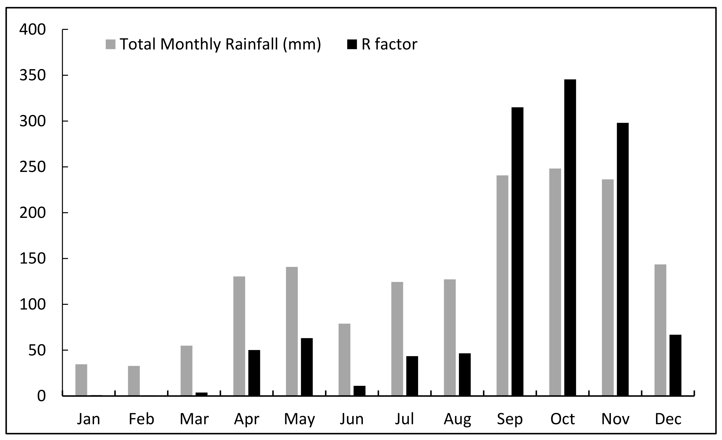
where Pi is the monthly rainfall in mm and P is the annual rainfall in mm. The annual average rainfall erosivity factor was observed to be 1245 MJ·mm·ha−1·h−1·y−1 when the total rainfall was 1593 mm in 96 rainy days. Figure 2 shows the temporal variation of total monthly rainfall and R factor, and indicates that rainfall-runoff erosivity is maximum during the north-east monsoon between September and November, and almost negligible during the winter months of January and February.
2.6. Soil Erodibility Factor (K)
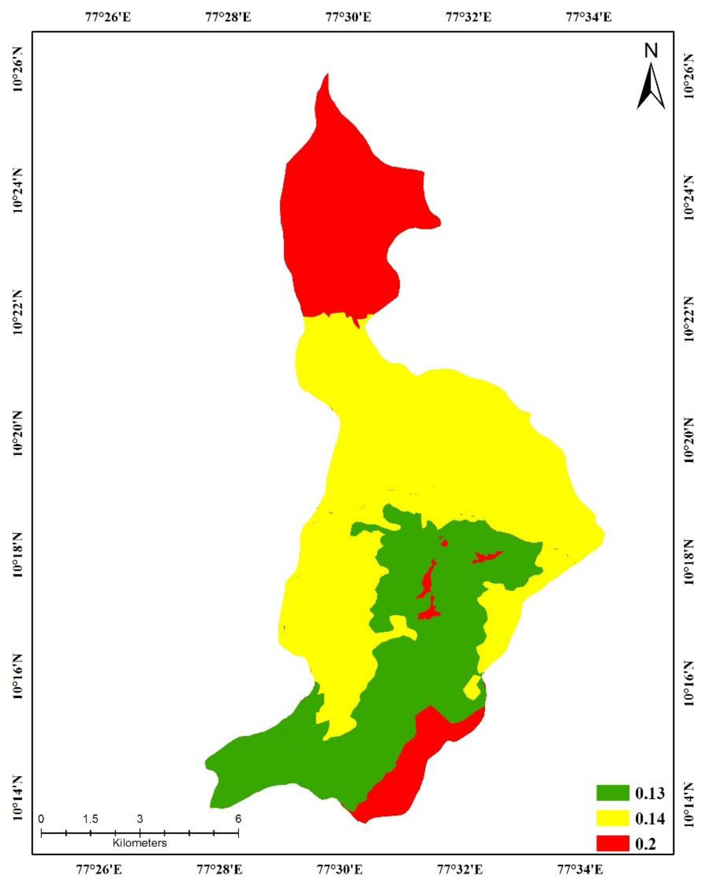
Erodibility of soil reflects its resistance to detachability and transport for a constant quantity and rate of runoff for a given rainfall, measured in a standard plot [17,30]. It is a function of intrinsic soil properties, such as texture, grain size, hydraulic conductivity of soil, the density of eroded soil, structure, organic content and cohesiveness [17]. Soil samples were collected from different locations in the site and were analyzed to determine the grain size distribution and organic content. A textural map was created from the field data, and three types of soil were identified in the region: sandy clay, sandy clay loam, and sandy loam. Samples showed very little or no cohesive strength and the average hydraulic conductivity of the soil ranged between 7.5 × 10⁻¹ cm/s for sand and 5 × 10⁻³ cm/s for fine sand and silt. In general, the organic content of the soil was very low (<2%). Minimum organic content in the soil samples indicates the greater susceptibility of the soil to erosion. The soil in the region was shallow to moderately deep and was well drained in general. K values were extracted from the soil erodibility nomogram [17] based on gradation, hydraulic conductivity, and organic content. These varied from 0.13 Mg·h·ha−1·MJ−1·mm−1 for sandy loam to 0.2 Mg·h·ha−1·MJ−1·mm−1 for sandy clay loam. Figure 3 shows the spatial variability of K factor in the Palar sub-watershed. A higher value of K indicates that the soil is more erodible, as it can be easily detached and results in high rates of runoff.
2.7. Slope Length and Steepness Factor (LS)
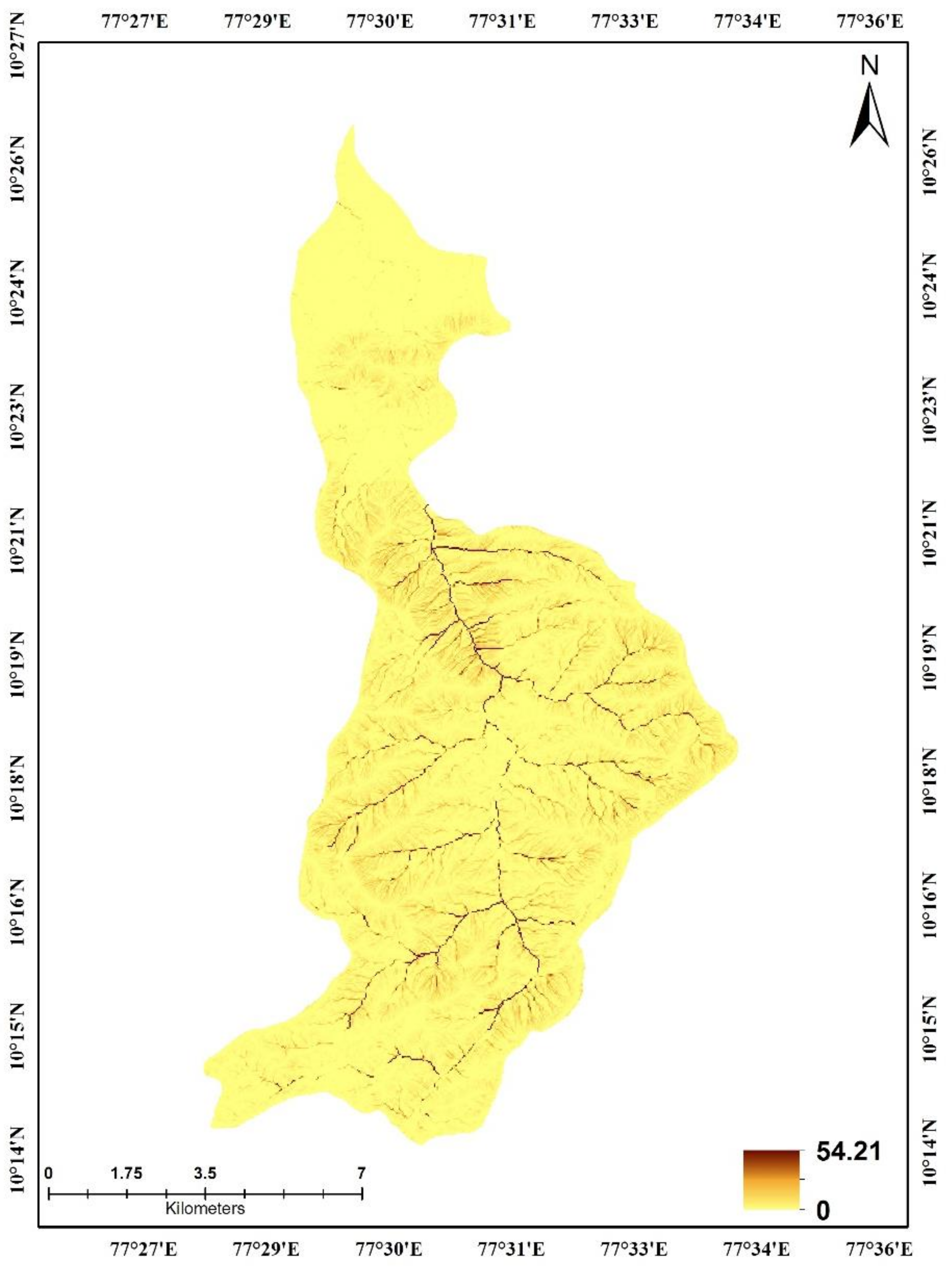
The topographic factor, or slope length and steepness factor (LS), accounts for the effect of the topography of the site on erosion. Soil erosion (total and per unit area) accelerates with the increase in the slope length as this causes progressive accretion of runoff in the downslope direction [31]. Similarly, velocity and erosivity of runoff intensify with the increase in slope steepness. RUSLE does not distinguish between rill and inter-rill erosion [1].
The slope of the watershed ranges from 0° to 65.73°, with a mean of 18.88° and standard deviation of 11.04°. Nearly 52% of the region has a moderate slope between 10° and 25°, and 7% of the area has an intensely undulating slope. Higher L values are observed where overland flow inclines to accrue in concave slopes and lower values in convex slopes where flow diverges [32]. The L values vary between 0 and 1164.79, with a mean of 7.11 and standard deviation of 51.8.
A combined topographic factor for the watershed was derived from a DEM using Arc Map following the approach of Moore and Burch [33,34]. Flow accumulation (representing the accumulated upslope contributing area for a given cell) and slope gradient (degrees) were calculated using the hydrology and ArcGIS spatial analyst extensions:
LS = (Flow accumulation × Cell Size/22.13)0.4 × {(Sin (slope) × 0.01745)/0.09}1.4
LS in the Palar watershed varied from 0 to 54.21 (Figure 4), with a mean of 0.11 and standard deviation of 0.57. Steeply sloping areas have a higher S value while gentle slopes have a higher L value. The mean LS reflects the gentle-moderate gradient of the majority of the watershed.
2.8. Crop Management Factor (C)
The crop management factor reflects the consequence of cropping and management practices, and disturbance to the natural environment (in terms of agriculture, productivity, crop sequence and length of growing season) and sub-surface biomass for soil loss erosion. The watershed is characterized by a variety of land cover practices, both in the spatial and temporal dimensions. Limited availability of land has resulted in smaller land holdings of farmers and little or no mechanization in agriculture. However, intense utilization of land resources, such as by continuous cropping, is evident. The land use and land cover map was prepared from the LANDSAT 8 satellite image at 30 m resolution and was used for assigning C values to generate the soil loss map. Table 1 depicts the C values adopted for the study.
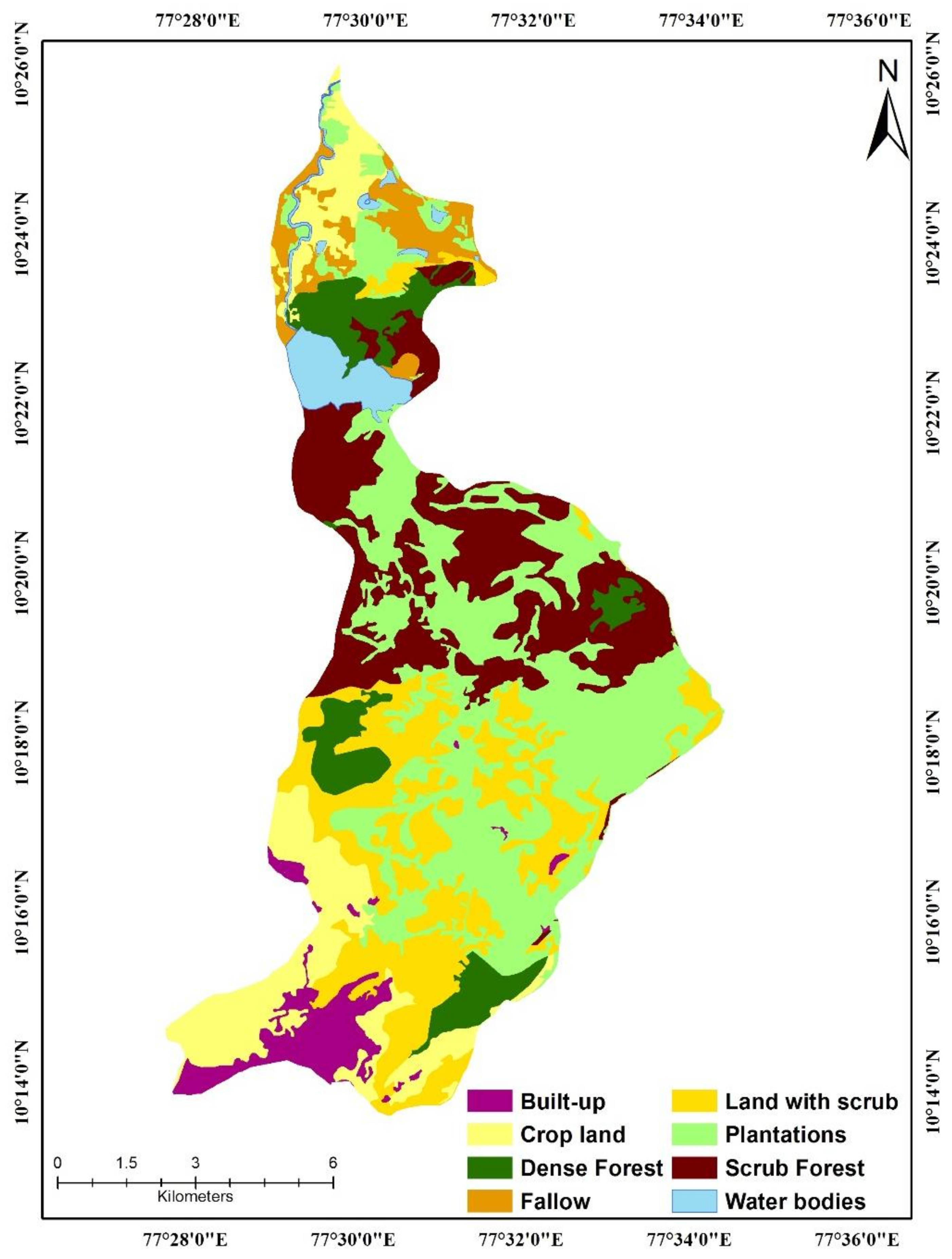
Predominant land cover types observed in the watershed are cropland and plantation categories. Scrub forests are significantly observed in the central region while settlements are abundant in the south. As a consequence, the crop factor is high in the central part and the northern fringe. The crop factor ranged between 0 and 1 (Figure 5).
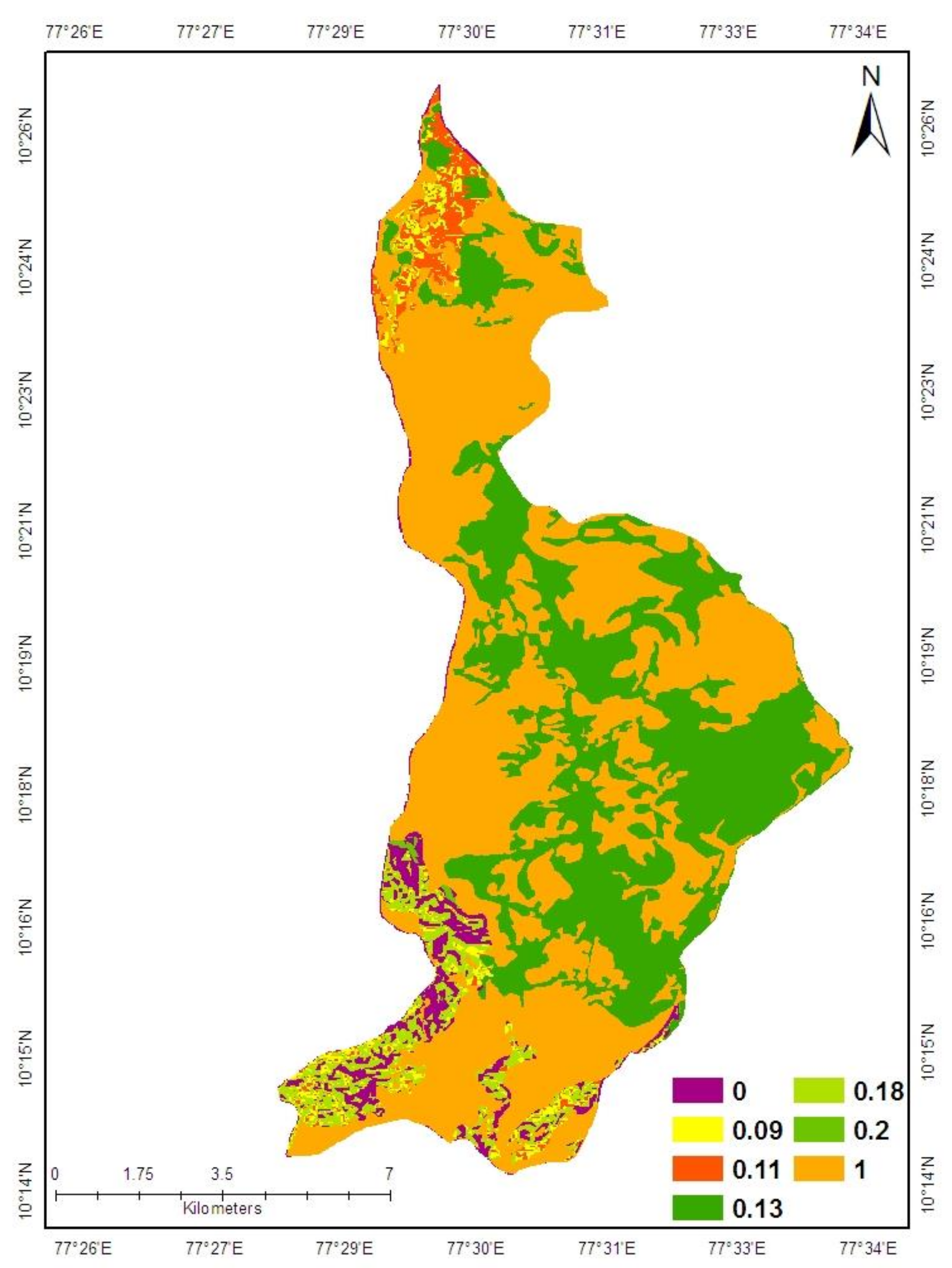
2.9. Conservation Support Practice Factor (P)
This factor associates the soil-loss ratio of a specific support practice to the corresponding soil loss with upslope and downslope tillage [1]. It showcases the effects of practices that alter the quantity and rate of runoff, with the consequence of reduced erosion [4,20,28,36]. The values of P ranged from 0 to 1; are assigned based on the study of Schwab et al. [37], after modification based on field observations (Table 2). Figure 6 shows the spatial distribution of the P factor in the watershed.
3. Spatial Distribution of Soil Loss, Validation and Sensitivity Analysis
3.1. Soil Loss Map
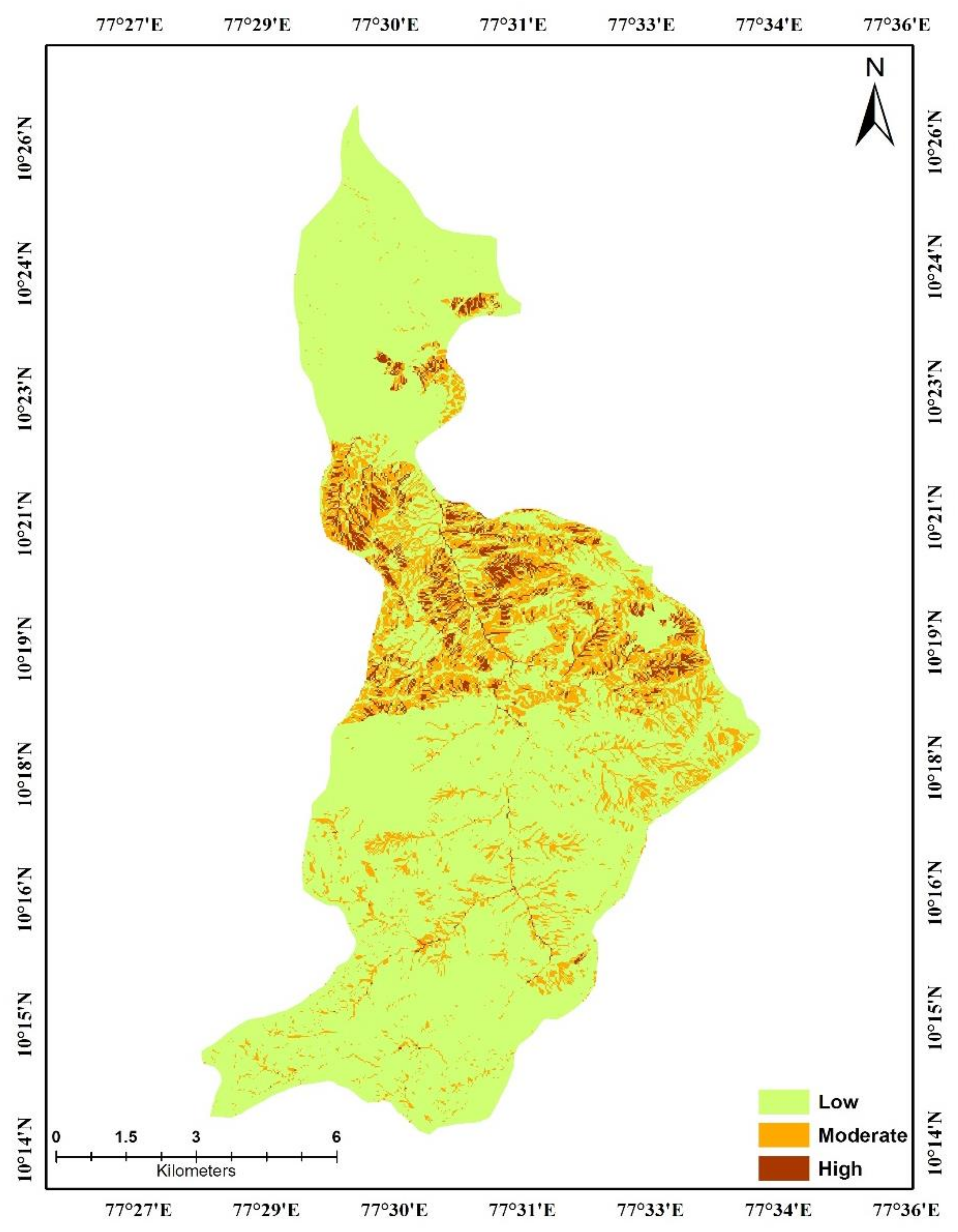
Annual soil loss is estimated using the RUSLE equation in a GIS environment by integrating the factors R, K, LS, C and P using raster operations. The resulting spatial distribution showed a maximum of 3345 Mg·ha−1·y−1, with a mean of 2.77 and standard deviation of 26.84. The high standard deviation and low mean indicated the large spread in the range of soil loss values. Only 0.27% of the area has a very high rate of soil erosion (i.e., greater than 100 Mg·ha−1·y−1), which applies to completely eroded peaks. These peaks are found usually in abandoned land with scrub forests and are in isolation. The relatively thin vegetative cover and predominantly granular soil found in the region aggravates the problem of erosion [38]. However, once the extreme values are filtered, the soil loss in the study area ranged between 0 and 118 Mg·ha−1·y−1. The quantitative soil loss in the Palar sub-watershed was classified into three ordinal classes: low (<1.5 Mg·ha−1·y−1), moderate (1.5–25 Mg·ha−1·y−1) and severe (>25 Mg·ha−1·y−1). Nearly 81% of the watershed fell within the low (tolerable) soil loss category, while 4% was classified to the severe erosion hazard category (Table 3). Figure 7 shows the spatial variation of soil loss in the watershed. The central part and northern fringes of the watershed were identified to be more prone to erosion. Severe erosion-prone zones contained a significant percent of scrub forests (wasteland), abandoned land that was covered with scrubs and pockets of plantations, while moderate erosion-prone areas were dominated by cropland and plantations.
3.2. Validation
To assess the applicability of the method for this watershed, the results of the study were compared with regions of similar geo-environment and climate in the Western Ghats [6,28,39] and found to be analogous. Soil loss was below 1.5 Mg·ha−1·y−1, for most of the watershed, which was considered in the low category. However, 4% of the area was classified to the severe category where the soil loss was greater than 25 Mg·ha−1·y−1, and the remaining area was between the low and severe categories. Limited field verification was also carried out to validate the results, which also ruled in favor of the application of the method to this watershed.
3.3. Sensitivity Analysis
Sensitivity analysis was performed to study the effect of the factors used to calculate the soil loss in the local geo-environment. The analysis showed that the rainfall erosivity factor (R) and topographic factor (LS) have a profound impact on the magnitude of soil loss (Table 4) and are found to be the significant factors controlling soil loss in this watershed. The distribution of the erosion zones shifted to the south of the study area with the removal of the factors K, C and P. In particular, a significant shift in the moderate zones occurred with the removal of LS, C or P. There was a considerable increase in the severely affected erosion zone with the removal of LS. The crop cover management factor and conservation support practice factor had the least effect on the magnitude of soil loss and K had the least effect on the distribution of erosion-prone areas. Table 4 shows statistical significance of each factor. The results of the sensitivity analysis showed that each of the factors have a significant role in the assessment of erosion in this watershed. Soil loss calculated by integration of all the factors was observed to be more complimentary to field observations.
4. Results and Discussion
Erosion damages the soil system and hence is a major threat to sustainability [40]. Diverse land management strategies are required to address the concerns that arise from soil loss in an agricultural area. The results of the study show that rainfall erosivity, slope steepness and soil erodibility factors are the important physical parameters that govern soil loss, but also that the quantum of soil loss is controlled by the land use patterns of the region.
The study area is characterized by high intensity of rainfall and vastly undulating terrain by virtue of its altitude. Also, the lithology is susceptible to detachment as it comprises primarily granular soil cover; that is, a mixture of sand, silt and clay with high hydraulic conductivity. All of these factors promote a high rate of soil loss. The area is characterized by moderate steepness, which also provides a greater impetus to soil loss. Hence, it can be summarized that the region is prone to heavy soil loss and that land use can either deter or promote the magnitude of soil loss.
The spatial distribution of soil loss reinforces the fact that land use patterns of the region play a crucial role in controlling the erosion process. The two land use categories of concern are scrub forests and abandoned land with sparse vegetation, where erosion is severe, and cropland and plantation, which show moderate susceptibility to soil erosion and soil loss. Nearly 79 acres of plantation, 1021 acres of waste land and 4.2 acres of cropland, where systematic agriculture was carried out by terrace cutting and irrigation, also falls within the severe erosion zone, i.e., regions where terrain modification was extensive. Nearly 22% (1930 acres) of the total area occupied by plantations and 7% (250 acres) of cropland fell within the moderate soil loss category (Figure 8). The presence of erosion in commercially important land cover categories, such as plantation and cropland, calls for conservation measures, not only in the interest of the environment but also for the economic sustainability of the region. The higher rates of erosion in these land cover categories are an indicator of anthropogenic interference and its influence on erosion.
Scrubs are ineffective in thwarting soil loss. The vegetative cover is sparse and a considerable expanse of soil is devoid of vegetative cover. The nature of soil in the region is predominantly sandy with little or no cohesion [26], which further leads to removal of soil cover without any resistance and higher infiltration rates. Slope steepness augments this process by providing momentum to sediment transport. Moderately steep slopes are more susceptible to soil erosion by water as steep slopes have a very limited but resistant soil cover/lithology and gentle slopes do not provide impetus to sediment transport by virtue of their gradinent. In contrast, moderately steep slopes support considerable soil overburden and also abet sediment movement. Land management strategies in these zones should aim at re-vegetation to decrease erosion. This would also increase infiltration of water into the soil and biological activity [41]. In order to impede soil loss, the literature also suggests simple techniques, such as straw covers [42], residues [43], grass cover [44], geotextiles [45] and organic amendments [46]. Revival of the native Shola grasslands can be very effective in controlling soil loss in these regions.
Intense agricultural activity compounds the magnitude of soil loss due to continued tillage, absence of vegetative cover that holds the soil, soil compaction, unsuitable irrigation practices, and use of herbicides and biocides that tends to reduce the biological activity. As a consequence, the process of soil formation is also impeded [47]. This sequence of factors makes agricultural lands susceptible to degradation, promotes soil loss and deters soil formation, and highlights the need to identify unsuitable land management practices that damage soil quality and impede sustainable agricultural uses of soil [13,38,48,49] Educating farmers on good agricultural practices such as the use of organic manures and pesticides, providing know-how on healthy irrigation methods like drip irrigation, and subsidies for good farming practices can help combat soil loss in agricultural lands and plantations. Terraces can be protected by hedgerow grasses like Napier grass (Pennisetum purpureum, family: Poaceae), Leucaenea leucocephala and asparagus [27]. Minimal severe erosion was noticed in built-up areas where slopes can be riveted with pebbles or stones to control soil wash off; asparagus grass can also be grown on these slopes. Awareness programs for local farmers on the impact of soil erosion on long-term agricultural productivity are necessary to effect a sustainable solution. These will help in restoring the health of the watershed and deter its degradation. Knowledge of zones prone to soil erosion in a watershed is therefore essential for assessing its environmental degradation, and to plan soil conservation strategies to combat soil loss and improve its health. The results of this study suggest that distributed soil erosion analysis using simple techniques can serve as a vital planning tool, particularly where the local economy is dependent on agriculture and pressures on land are very high owing to rapid urbanization, as in this case. This awareness can enhance the understanding of the limitations of the terrain and, hence, play a major role in regional and local land use planning and management with sustainable development as a theme. At the planning stage, this is an effective and economic option.
5. Conclusions
The study brings to light the severity and impact of erosion in the Palar sub-watershed in the Western Ghats. Annual soil loss was estimated using the RUSLE empirical model in a spatial environment with the help of GIS. The study proves the usefulness of remotely sensed data in deriving the inputs for the RUSLE model, making the study cost efficient and practical, given the constraints of data from the region. The results of the study showed that all the factors—namely, R, K, LS, C and P—play a significant role in assessing the erosion potential of the region. The general undulating nature of the terrain and high drainage density provides the impetus for rapid removal of soil under the erosive effect of rainfall. Erosion was found to be severe in the central part of the watershed and its northern fringes. Scrub forests and waste lands appeared to accentuate soil loss. Erosion was also significant in plantations. This could be attributed to shifting agriculture and unhealthy agricultural practices; e.g., natural forests have been replaced with eucalyptus plantations and orchards. Terrain modification, particularly in the form of croplands and degradation of forests, also adds to the problem of erosion. The health of the watershed can be improved by restoring the native Shola grasslands, which are very effective in controlling erosion, particularly on steep terrain. The erosion hazard map can be a vital tool for watershed development and also help in local and regional planning.
Author Contributions
Formal analysis, E.R.S.; Investigation, E.R.S.; Methodology, V.S.; Project administration, V.S.; Supervision, V.S.; Writing—original draft, E.R.S.; Writing—review & editing, V.S.
Funding
This project was funded, in part for the corresponding author, by the Virginia Agricultural Experiment Station (Blacksburg) and the Hatch Program of the National Institute of Food and Agriculture, U.S. Department of Agriculture (Washington, D.C.). We are also thankful for the financial support from Virginia Tech’s Open Access Subvention Fund.
Acknowledgments
We would like thank the Vice Chancellor, SASTRA University and Kumar Mallikarjunan, Department of Food Science and Nutrition, University of Minnesota for facilitating the faculty collaboration.
Conflicts of Interest
The authors declare no Conflict of Interest.
References
- Renard, K.G.; Foster, G.R.; Weesies, G.A.; McCool, D.K.; Yoder, D.C. Predicting Soil Erosion by Water: A Guide to Conservation Planning with the Revised Universal Soil Loss Equation (RUSLE); Agriculture Handbook; US Department of Agriculture: Washington, DC, USA, 1997; Volume 703, pp. 1–251.
- Boyle, M. Erosion’s contribution to greenhouse gases. Eros. Control 2002, 9, 21–29. [Google Scholar]
- Narayan, V.V.D.; Babu, R. Estimation of soil erosion in India. J. Irrig. Drain. Eng. 1983, 109, 419–434. [Google Scholar] [CrossRef]
- Dabral, P.P.; Baithuri, N.; Pandey, A. Soil erosion assessment in a hilly catchment of North Eastern India using USLE, GIS and remote sensing. Water Resour. Manag. 2008, 22, 1783–1798. [Google Scholar] [CrossRef]
- Pandey, A.; Mathur, A.; Mishra, S.K.; Mal, B.C. Soil erosion modeling of a Himalayan watershed using RS and GIS. Environ. Earth Sci. 2009, 59, 399–410. [Google Scholar] [CrossRef]
- Prasannakumar, V.; Shiny, R.; Geetha, N.; Vijith, H. Spatial prediction of soil erosion risk by remote sensing, GIS and RUSLE approach: A case study of Siruvani river watershed in Attapady valley, Kerala, India. Environ. Earth Sci. 2011, 64, 965–972. [Google Scholar] [CrossRef]
- Sharma, A. Integrating terrain and vegetation indices for identifying potential soil erosion risk area. Geol. Spat. Inf. Sci. 2010, 13, 201–209. [Google Scholar] [CrossRef] [Green Version]
- Angima, S.D.; Stott, D.E.; O’Neill, M.K.; Ong, C.K.; Weesies, G.A. Soil erosion prediction using RUSLE for central Kenyan highland conditions. Agric. Ecosyst. Environ. 2003, 97, 295–308. [Google Scholar] [CrossRef]
- Xu, Y.; Zhou, Q.; Li, S. An analysis on spatial–temporal distribution of rainfall erosivity in Guizhou Province. Bull. Soil Water Conserv. 2005, 4, 11–14. [Google Scholar]
- Xu, Y.-Q.; Peng, J.; Shao, X.-M. Assessment of soil erosion using RUSLE and GIS: A case study of the Maotiao river watershed, Guizhou Province, China. Environ. Geol. 2009, 56, 1643–1652. [Google Scholar]
- Keesstra, S.D.; Temme, A.J.A.M.; Schoorl, J.M.; Visser, S.M. Evaluating the hydrological component of the new catchment-scale sediment delivery model LAPSUS-D. Geomorphology 2014, 212, 97–107. [Google Scholar] [CrossRef]
- Pandey, A.; Himanshu, S.K.; Mishra, S.K.; Singh, V.P. Physically based soil erosion and sediment yield models revisited. CATENA 2016, 147, 595–620. [Google Scholar] [CrossRef]
- Mekonnen, M.; Keesstraa, S.D.; Baartmana, J.E.M.; Stroosnijdera, L.; Maroulisac, J. Reducing sediment connectivity through man-made and natural sediment sinks in the Minizr Catchment, Northwest Ethiopia. Land Degrad. Dev. 2016, 28, 708–717. [Google Scholar] [CrossRef]
- Guzmán, G.; Quinton, J.N.; Nearing, M.A.; Mabit, L.; Gómez, J.A. Sediment tracers in water erosion studies: Current approaches and challenges. J Soils Sediments 2013, 13, 816–833. [Google Scholar] [CrossRef]
- Masselink, R.J.H.; Temme, A.J.A.M.; Giménez, R.; Casalí, J.; Keesstra, S.D. Assessing hillslope-channel connectivity in an agricultural catchment using rare-earth oxide tracers and random forests models. Cuadernos de Investigación Geográfica 2017, 43, 19–39. [Google Scholar] [CrossRef]
- Temme, A.J.A.M.; Claessens, L.; Veldkamp, A.; Schoorl, J.M. Evaluating choices in multi-process landscape evolution models. Geomorphology 2011, 125, 271–281. [Google Scholar] [CrossRef]
- Wischmeier, W.H.; Smith, D.D. Predicting Rainfall Erosion Losses: A Guide to Conservation Planning; Agriculture Handbook No. 537; US Department of Agriculture Science and Education Administration: Washington, DC, USA, 1978.
- Nearing, M.A.; Foster, G.R.; Lane, L.J.; Finkner, S.C. A process-based soil erosion model for USDA Water Erosion Prediction Project technology. Trans. ASABE 1989, 32, 1587–1593. [Google Scholar] [CrossRef]
- Morgan, R.P.C.; Quinton, J.N.; Smith, R.E.; Govers, G.; Poesen, J.W.A.; Auerswald, K.; Chisci, G.; Torri, D.; Styczen, M.E. The European Soil Erosion Model (EUROSEM): A dynamic approach for predicting sediment transport from fields and small catchments. Earth Surf. Proc. Landf. 1998, 23, 527–544. [Google Scholar]
- Ganasiri, B.P.; Ramesh, H. Assessment of soil erosion by RUSLE model using remote sensing and GIS—A case study of Nethravathi Basin. Geosci. Front. 2016, 7, 953–961. [Google Scholar] [CrossRef]
- Bhandari, K.P.; Aryal, J.; Darnsawasdi, R. A geospatial approach to assessing soil erosion in a watershed by integrating socio-economic determinants and the RUSLE model. Nat. Hazards 2015, 75, 321–342. [Google Scholar] [CrossRef]
- Kouli, M.; Soupios, P.; Vallianatos, F. Soil erosion prediction using the Revised Universal Soil Loss Equation (RUSLE) in a GIS framework, Chania, Northwestern Crete, Greece. Environ. Geol. 2009, 57, 483–497. [Google Scholar] [CrossRef]
- Shrestha, D.P. Assessment of soil erosion in the Nepalese Himalaya, a case study in Likhu Khola Valley, middle mountain region. Land Husb. 1997, 2, 59–80. [Google Scholar]
- Van De, N.; Douglas, I.; McMorrow, J.; Lindley, S.; Binh, D.K.N.T.; Van, T.T.; Tho, N. Erosion and nutrient loss on sloping land under intense cultivation in southern Vietnam. Geogr. Res. 2008, 46, 4–16. [Google Scholar] [CrossRef]
- Prasuhn, V. Soil erosion in the Swiss midlands: Results of a 10-year field survey. Geomorphology 2011, 126, 32–41. [Google Scholar] [CrossRef]
- Sujatha, E.R.; Sridhar, V. Mapping Debris Flow Susceptibility using Analytical Network Process in Kodaikkanal Hills, Tamil Nadu (India). J. Earth Syst. Sci. 2017, 112, 116. [Google Scholar] [CrossRef]
- Sujatha, E.R.; Rajamanickam, G.V. Landslide Hazard and Risk Mapping using Weighted Linear Combination Applied to Tevankarai Stream Watershed, Kodaikkanal, India. Hum. Ecol. Risk Assess. J. 2015, 21, 1445–1461. [Google Scholar] [CrossRef]
- Prasannakumar, V.; Vijith, H.; Abinod, S.; Geetha, N. Estimation of soil erosion risk within a small mountainous subwatershed in Kerala, India, using Revised Universal Soil Loss Equation (RUSLE) and geo-information technology. Geosci. Front. 2012, 3, 209–215. [Google Scholar] [CrossRef]
- Arnoldus, H.M.J. An approximation of the rainfall factor in the Universal Soil Loss Equation. In Assessment of Erosion; De Boodt, M., Gabriels, D., Eds.; Wiley: Hoboken, NJ, USA, 1980; pp. 127–132. [Google Scholar]
- Schwab, G.O.; Frevert, R.K.; Edminster, T.W.; Barner, K.K. Soil and Water Conservation Engineering, 3rd ed.; John Wiley & Sons: New York, NY, USA, 1981; p. 525. [Google Scholar]
- McCool, D.K.; Brown, L.C.; Foster, G.R. Revised slope steepness factor for the universal soil loss equation. Trans. ASABE 1987, 30, 1387–1396. [Google Scholar] [CrossRef]
- Hoyos, N. Spatial modeling of soil erosion potential in a tropical watershed of the Colombian Andes. CATENA 2005, 63, 85–108. [Google Scholar] [CrossRef]
- Moore, I.D.; Burch, G.J. Physical basis of the length slope factor in the universal soil loss equation. Soil Sci. Soc. Am. J. 1986, 50, 1294–1298. [Google Scholar] [CrossRef]
- Moore, I.D.; Burch, G.J. Modelling erosion and deposition topographic effects. Trans. ASABE 1986, 29, 1624–1630. [Google Scholar] [CrossRef]
- Hashim, G.M.; Wong, N.C. Erosion from Steep Land under Various Plant Cover and Terrains; Tay, T.H., Mokhtaruddin, A.M., Zahari, A.B., Eds.; MARDI/Malaysian Society of Soil Science: Kuala Lumpur, Malaysia, 1988; pp. 424–461. [Google Scholar]
- Al-Quraishi, A.M.F. Soil erosion risk prediction with RS and GIS for the northwestern part of Hebei Province, China. Pak. J. Appl. Sci. 2003, 3, 659–669. [Google Scholar]
- Schwab, G.; Frevert, R.; Dminster, T.; Barnes, K. Soil and Water Conservation Engineering, 2nd ed.; The Fergunson Foundation Agricultural Engineering Series; John Wiley & Sons: New York, NY, USA, 1966; p. 683. [Google Scholar]
- Martínez-Hernández, C.; Rodrigo-Comino, J.; Romero-Díaz, A. Impact of lithology and soil properties on abandoned dry-land terraces during the early stages of soil erosion by water in Southeast Spain. Hydrol. Process. 2017, 31, 3095–3109. [Google Scholar] [CrossRef]
- Matsuura, H. Design Guidelines for Mechanical Soil and Water Conservation Works and Water Resources Development; Technical Report for the Attapady Wasteland Comprehensive Environmental Conservation Project (AWCECOP), ID-P111; Attapady Hills Area Development Society, Government of Kerala: Kerala, India, 2000.
- Cerdà, A.; Rodrigo-Comino, J.; Giménez-Morera, A.; Novara, A.D.; Pulido, M.; Kapović-Solomun, M.; Keesstra, S.D. Policies can help to apply successful strategies to control soil and water losses. The case of chipped pruned branches (CPB) in Mediterranean citrus plantations. Land Use Policy 2018, 75, 734–745. [Google Scholar] [CrossRef] [Green Version]
- Bienes, R.; Marques, M.J.; Sastre, B.; García-Díaz, A.; Ruiz-Colmenero, M. Eleven years after shrub revegetation in semiarid eroded soils. Influence in soil properties. Geoderma 2016, 273, 106–114. [Google Scholar] [CrossRef]
- Cerdà, A.; González-Pelayo, Ó.; Giménez-Morera, A.; Jordán, A.; Pereira, P.; Novara, A.; Brevik, E.C.; Prosdocimi, M.; Mahmoodabadi, M.; Keesstra, S.; et al. Use of barley straw residues to avoid high erosion and runoff rates on persimmon plantations in eastern Spain under low frequency—High magnitude simulated rainfall events. Soil Res. 2016, 54, 154–165. [Google Scholar] [CrossRef]
- Prosdocimi, M.; Jordán, A.; Tarolli, P.; Keesstra, S.; Novara, A.; Cerdà, A. The immediate effectiveness of barley straw mulch in reducing soil erodibility and surface runoff generation in Mediterranean vineyards. Sci. Total Environ. 2016, 547, 323–330. [Google Scholar] [CrossRef] [PubMed] [Green Version]
- Novara, A.; Gristina, L.; Saladino, S.S.; Santoro, A.; Cerdà, A. Soil erosion assessment on tillage and alternative soil managements in a Sicilian vineyard. Soil Tillage Res. 2011, 117, 140–147. [Google Scholar] [CrossRef] [Green Version]
- Giménez-Morera, A.; Ruiz-Sinoga, J.D.; Cerdà, A. The impact of cotton geotextiles on soil and water losses from Mediterranean rainfed agricultural land. Land Degrad. Dev. 2010, 21, 210–217. [Google Scholar] [CrossRef]
- Hueso-Gonzalez, P.; Ruiz-Sinoga, J.; Martínez-Murillo, J.; Lavee, H. Overland flow generation mechanisms affected by topsoil treatment: Application to soil conservation. Geomorphology 2015, 228, 796–804. [Google Scholar] [CrossRef]
- Brevik, E.C.; Fenton, T.E. Long-term effects of compaction on soil properties along the Mormon trail, South-Central Iowa, USA. Soil Horiz. 2012, 53, 37–42. [Google Scholar] [CrossRef]
- Mhazo, N.; Chivenge, P.; Chaplot, V. Tillage impact on soil erosion by water: Discrepancies due to climate and soil characteristics. Agric. Ecosyst. Environ. 2016, 230, 231–241. [Google Scholar] [CrossRef]
- Rodrigo-Comino, J.; Brings, C.; Iserloh, T.; Casper, C.M.; Seeger, M.; Senciales, M.; Brevik, E.C.; Ruiz-Sinoga, J.D.; Ries, J.B. Temporal changes in soil water erosion on sloping vineyards in the Ruwer-Mosel Valley. The impact of age and plantation works in young and old vines. J. Hydrol. Hydromech. 2017, 65, 402–409. [Google Scholar] [CrossRef]
Figure 1.
Map of the study area from a digital elevation model, with a maximum altitude of 2346 m above mean sea level.
Figure 1.
Map of the study area from a digital elevation model, with a maximum altitude of 2346 m above mean sea level.

Figure 2.
Temporal variation of rainfall erosivity (R) factor.

Figure 3.
Spatial variation of soil erodibility (K) factor.

Figure 4.
Topographic factor (LS) describing the effect of slope length and steepness.

Figure 5.
Crop management factor (C).

Figure 6.
Conservation support practice factor (P).

Figure 7.
Spatial distribution of erosion classes.

Figure 8.
Land use and land cover distribution in Palar sub-watershed.


| Land Cover | Average C Value | Land Cover | Average C Value |
|---|---|---|---|
| Open Forest | 0.05 | Scrub | 0.01 |
| Built-Up Land | 0.05 | Dense Forest | 0.001 |
| Cropland | 0.45 | Planation | 0.05 |
| Water Bodies | 0.00 | Barren Land | 1.00 |
Table 2.
Adopted P factor values (after Schwab et al. [37] and modified based on field survey).
Table 2.
Adopted P factor values (after Schwab et al. [37] and modified based on field survey).
| Land Use | Slope (°) | Conservation Support Practice Factor (P) |
|---|---|---|
| Agriculture | 1–4 | 0.11 |
| 5–10 | 0.09 | |
| 11–20 | 0.18 | |
| 21–40 | 0.00 | |
| >40 | 0.20 | |
| Plantation | All | 0.13 |
| All | 1.00 |
Table 3.
Soil loss distribution in the Palar sub-watershed.
| Description | Soil Loss (Mg·ha−1·y−1) | Area (Hectares) | % Area |
|---|---|---|---|
| Low | 0–1.5 | 8798 | 81 |
| Moderate | 1.5–25 | 1624 | 15 |
| Severe | >25 | 435 | 4 |
Table 4.
Sensitivity analysis of factors used in RUSLE model.
| Description | Minimum | Maximum | Mean | Standard Deviation |
|---|---|---|---|---|
| Removal of R | 0 | 2.68 | 0.0022 | 0.022 |
| Removal of K | 0 | 23.898 | 19.298 | 191.22 |
| Removal of LS | 0 | 249.11 | 35.39 | 69.46 |
| Removal of C | 0 | 3558.55 | 7.53 | 44.58 |
| Removal of P | 0 | 3345.85 | 3.196 | 27.62 |
© 2018 by the authors. Licensee MDPI, Basel, Switzerland. This article is an open access article distributed under the terms and conditions of the Creative Commons Attribution (CC BY) license (http://creativecommons.org/licenses/by/4.0/).
Share and Cite
MDPI and ACS Style
Sujatha, E.R.; Sridhar, V. Spatial Prediction of Erosion Risk of a Small Mountainous Watershed Using RUSLE: A Case-Study of the Palar Sub-Watershed in Kodaikanal, South India. Water 2018, 10, 1608. https://doi.org/10.3390/w10111608
AMA Style
Sujatha ER, Sridhar V. Spatial Prediction of Erosion Risk of a Small Mountainous Watershed Using RUSLE: A Case-Study of the Palar Sub-Watershed in Kodaikanal, South India. Water. 2018; 10(11):1608. https://doi.org/10.3390/w10111608
Chicago/Turabian StyleSujatha, Evangelin Ramani, and Venkataramana Sridhar. 2018. "Spatial Prediction of Erosion Risk of a Small Mountainous Watershed Using RUSLE: A Case-Study of the Palar Sub-Watershed in Kodaikanal, South India" Water 10, no. 11: 1608. https://doi.org/10.3390/w10111608
Note that from the first issue of 2016, this journal uses article numbers instead of page numbers. See further details here.