Quantifying the Relationship between Drought and Water Scarcity Using Copulas: Case Study of Beijing–Tianjin–Hebei Metropolitan Areas in China


1
State Key Laboratory of Simulation and Regulation of Water Cycle in River Basin, China Institute of Water Resources and Hydropower Research, Beijing 100083, China
2
Beijing Key Laboratory of Urban Hydrological Cycle and Sponge City Technology, College of Water Sciences, Beijing Normal University, Beijing 100875, China
3
Agricultural Water Conservancy Department, Changjiang River Scientific Research Institute, Wuhan 430015, China
*
Author to whom correspondence should be addressed.
Water 2018, 10(11), 1622; https://doi.org/10.3390/w10111622
Submission received: 18 September 2018
/
Revised: 29 October 2018
/
Accepted: 7 November 2018
/
Published: 9 November 2018
(This article belongs to the Section Water Resources Management, Policy and Governance)
Abstract
:Making the distinction between drought and water scarcity is not trivial, because they often occur simultaneously. In this study, we used Copulas to quantify the relationship between drought and water scarcity. Beijing–Tianjin–Hebei Metropolitan Areas (BTHMA) was chosen as the study area. Standard Precipitation and Evapotranspiration Index (SPEI) and water exploitation index plus (WEI+) was chosen to represent metrological drought and water scarcity. Inverse Distance Weighted method was used for spatial analysis of SPEI and WEI+, and Archimedean Copula was used to establish two-dimensional joint probability distribution of SPEI and WEI+. The results are as follows: (1) The southern part of the study area was wetter. The middle part was drier, with moderate drought happened for most times. (2) WEI+ of Beijing and Tianjin showed significant decreasing trends from 2000 to 2015, while WEI+ of Hebei Province did not, which indicated that Hebei Province is facing much severer water scarcity situation than Beijing and Tianjin. (3) Gumbel copula was the best-fitting model to establish the joint probability distribution of SPEI and WEI+. The condition probability provided a probability distribution of water scarcity under different drought conditions, which can provide technical support for government managers during policy making.
1. Introduction
Water represents an essential element for the life of all who inhabit our planet [1]. Drought and water scarcity are two phenomena closely related to water quantity issues, and usually have influences on the society. Drought is defined as a natural temporary imbalance in water availability, which may be related to persistently lower-than-average precipitation [2]. Droughts have uncertain frequencies, durations and severities, and their occurrence is difficult to predict. Water scarcity is defined as the relative shortage of water in a water supply system which can be caused by drought or by human actions [3]. This is an imbalance of water supply and demand [4]. Although the terms ‘‘water scarcity’’ and ‘‘drought’’ are often used interchangeably, they refer to quite different phenomena [5]. Efforts have been taken to distinct drought and water scarcity since it matters for water management. The European Commission (EC) Expert Group on Water Scarcity and Drought held several meetings, aimed at making the distinction between drought and water scarcity [6]. Table 1 illustrates the differences between drought and water scarcity in several aspects, according to Strosser et al. [7].
It is rather important to distinguish drought and water scarcity, especially for water resources management, in order to avoid potential wrong decision making. The effects of water management measurements on these two phenomena are quite different. Management measurements can effectively alleviate the overuse of water resources, thus resolving the problem of water scarcity. However, management measurements can only adapt to the drought situation by decreasing vulnerability and increasing resilience [5,13,14]. It is common that both drought and water scarcity occur at the same time, that is, in water scarcity regions, the influence of drought on society would be much worse. Under such condition, it is crucial for policy makers to distinguish these two terms and understand the relationship between the two phenomena.
Studies have been focused on the interaction of drought and water scarcity qualitatively by using different indicators. Mazzanti et al. [15] applied both drought index SPEI (Standard Precipitation and Evapotranspiration Index), SRI (Standard Runoff Index), and water scarcity index WEI+ (Water Exploitation Index Plus) to explore the relationship between drought and water scarcity in Po and Arno River Basin, Italy. They found it is rather important to consider water availability when analysing drought. Kossida and Mimikou [16] calculated the DVI (drought vulnerability index) in Pinios River Basin, Greek. Then they drew a new risk map of DVI value combined with underground water development, water scarcity, land use and other social economic data. The new risk map was a compound map considering both drought and water scarcity situation, thus can help decision makers better identify the priority region. Other studies tried to give quantitative results between drought and water scarcity. Van Lanen et al. [17] used a large-scale hydrological model to predict future drought characteristics (such as severity and duration), then they calculated the probability of water scarcity, which may be caused by future drought. Van Loon and Van Lanen [5] proposed an observation-modelling framework to make the distinction. They quantified the distinction between drought (natural effects) and water scarcity (human effects) based on the conceptual hydrological model HBV (Hydrologiska Byråns Vattenbalansavdelning model). Followed the observation-modelling framework established by Van Looe and Van Lanen, Chen and Li [18] applied this framework to Luanhe River Basin, China to separate drought and water scarcity.
This paper attempts to quantify the relationship between drought and water scarcity through different drought and water scarcity indicators, based on their joint probability distribution, which is established using copulas. Copulas use a nonlinear approach to establish the joint probability distribution of two or more related variables and are able to model the dependence structure between random variables independent of their marginal distributions. In this paper, we chose Beijing–Tianjin–Hebei metropolitan areas (BTHMA) as the study area. We used SPEI to represent drought, and WEI+ to represent water scarcity. Copulas were applied to establish the joint and conditional probability distribution between SPEI and WEI+. From the joint and conditional probability distribution, the risk for future water scarcity under different drought situation can be obtained.
2. Materials and Methods
2.1. Study Area and Data
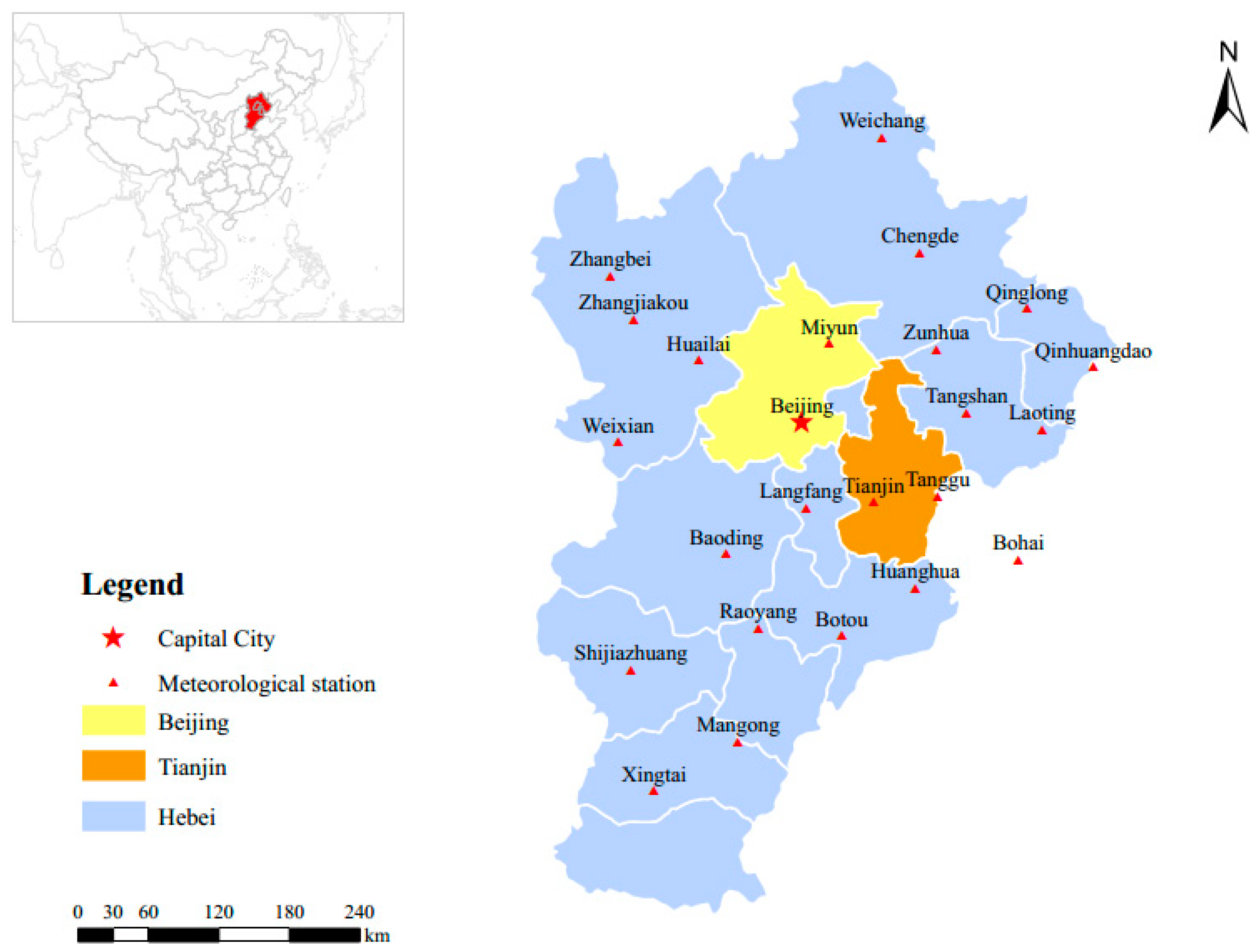
Beijing–Tianjin–Hebei metropolitan areas (BTHMA), located in northeast part of China, are consist of Beijing, Tianjin and Heber Province. BTHMA is the most important political, economic and cultural centre of China. Since it locates in northeast part of China, it is regarded was a water-stressed area. So, drought and water scarcity have become important factors for sustainable development of BTHMA.The study area comprises roughly 222,000 km2, accounting for only 2% of the total area of China. Yet the population in this area reaches 111.5 million, accounting for more than 8% of the total population in China. Southeast of BTHMA is mainly flat, while its northern areas consist of plateaus and mountains. The geographic features affecting the climate of BTHMA are the Inner Mongolia Plateau, the Hubei Plains, and the Bohai Sea [19]. The climate type of this area is temperate semi-humid semi-arid continental monsoon climate. Affected by the East Asian monsoon circulation and the mid-high and low latitude weather system activities, the annual precipitation is very uneven distributed in space and time. On average the maximum precipitation occurs in July and August and the minimum in February.
The SPEI was used to represent meteorological drought. Monthly total precipitation (mm) and monthly mean temperature (°C) data were collected from 24 meteorological stations which have continuous record were acquired from meteorological data sharing service system of China (http://cdc.cma.gov.cn). The investigated time series were selected according to the availability and reliability of the data sets. Thus, a record length of 64 years (1951–2015) was considered, which is the maximum time period of precipitation data recorded covering all the 24 synoptic stations. The main information about the stations is presented in Table 2 and the geographical set of the stations is shown in Figure 1.
The WEI+ index was used to represent water scarcity situation. Such data as total amount of water resources, inflow and outflow, water supply and water consumption, reservoir impoundment change used for calculating WEI+ index were collected from Water Resources Bulletin of Beijing, Tianjin and Hebei Province during 2001–2015.
2.2. SPEI
The calculation process for SPEI was described by Vicente-Serrano et al. [9], following three steps.
Step1: Calculate the water balance D series for month j, and obtain the accumulated D series at different time scale.
where P is monthly total precipitation, PET is potential evapotranspiration. In this paper, PET is calculated using the Thornthwaite method, requiring only monthly precipitation and temperature data [20]. The calculated values are aggregated at different time scales, forming Xijk series. K is the time scale, which could be 3, 6, 12 or 24 months, for both seasonal and annual drought analysis. So Xijk represents the accumulated water deficient in year i, month j, under time scale k. The difference in month j and year i depends on the chosen time scale k.
Step 2: Use a three-parameter log-logistic probability density function to fit the established X series. Then, obtain the cumulative probability function as follows:
where f(x) is the probability density function of X series; F(x) is the probability distribution function of X series; and α, β, and γ are scale, shape, and origin parameters, respectively, for D values, which can be obtained using an L-moments approach.
Step 3: Obtain the SPEI as the standardized values of F(x):
where P is the probability of exceeding a determined X value and P = 1 − F(x). If P > 0.5, then P is replaced by 1 − P, and the sign of the resultant SPEI is reversed. The constants are as follows: C0 = 2.515517, C1 = 0802853, C2 = 0.010328, d1 = 1.432788, d2 = 0.189269, and d3 = 0.001308.
2.3. WEI+
The Water Exploitation Index Plus (WEI+) is improved from the original Water Exploitation Index (WEI). Traditionally the WEI has been defined as the annual total water abstraction as a percentage of available long-term freshwater resources. The WEI can reflect the level of pressure that human activity exerts on the natural water resources of a particular territory, helping to identify those prone to suffer problems of water stress [11]. The WEI has been calculated so far for mainly on a national basis. In 2012, the Expert Group on Water Scarcity & Drought from EU has updated WEI into WEI+ with the purpose of better capturing the balance between renewable water resources and water consumption, in order to assess the prevailing water stress conditions in a river basin. WEI+ would be formulated in the following term:
where, AB is short for Abstractions, it refers the total amount of water abstracted from the river basin, including both surface water resources and groundwater resources. RE is short for Returns, it refers to the amount of water returning to the hydrological cycle after being used by human activities. RWR is short for renewable water resource. For river basin with or without human interventions, there are different methods for calculating renewable water resources.
For natural river basin, there are two options for calculating renewable water resources:
Option 1:
Option 2:
In this case, ExIn (Actual External Inflow) is the total volume of actual flow of rivers and groundwater, coming from neighbouring territories. P (Precipitation) is the total volume of atmospheric wet precipitation (rain, snow, hail), usually measured by meteorological or hydrological stations. Eta (Actual Evapotranspiration) is the total volume of evaporation from the ground, wetlands and natural water bodies and transpiration of plants. ∆S is the change of the stored amount of water during the given time period. When the time period is defined as long-term average, then ∆S can be ignored. Qnat is the natural runoff from the region, including both flowing to neighbor regions and flowing to the sea.
For river basin that is influenced by human activities, the observed runoff of the river export is not equal to the renewable water resources of the river basin. So RWR should be calculated in the following two options.
Option 1:
Option 2:
In this case, is the change of the stored amount of water in natural environment, including river beds, natural lakes, and underground water (soil moisture and groundwater). is the change of stored amount of water in regulated lakes or artificial reservoirs. Outflow is the actual outflow of the river basin, which should be distinguished from Qnat.
The threshold of WEI+ can be referred to as the threshold of WEI. According to literature, the warning threshold for WEI can be 40%, which distinguishes a non-stressed region from a stressed region [22,23]. Experts argued that if WEI reaches over 40%, then the whole ecosystem cannot remain healthy [24]; therefore, a threshold of 40% is used for WEI+ in this study.
2.4. Copula Model and Conditional Probability Distribution
2.4.1. Copula Model
Copula theory was first introduced by Sklar [25], and then developed by Nelson [26], making copulas powerful tools for establishing multivariate joint distributions and analysing the correlation between different variables. In this paper, Gumbel, Frank and Clayton copulas, all belong to Archimedean copulas, were chosen to match the two variables (SPEI and WEI+). The cumulative distribution functions (CDF) of the Gumbel, Frank and Clayton copulas are described in Equations (12) to (14) [27]:
Gumbel:
Frank:
Clayton:
where u and v are two variables, and θ is the copula parameter. τ is the Kendall rank correlation coefficient, which can be calculated using Equation (15):
where sgn is the sign function, n is the number of samples, and (di, si) is the actual data.
Four criterions, namely Ordinary least squares (OLS), mean square error (MSE) [28], Akaike information criterion (AIC) [29], and Bayesian information criterion (BIC) [30] were used to assess the fitting results of different copulas and to identify the best-performing one. The minimum value reflects the best-fitting result. The OLS, MSE, AIC, and BIC measures were defined as follows:
where Pei is the empirical frequency, Pi is the theoretical frequency, m is the number of copula parameters, and n is the number of samples.
2.4.2. Conditional Probability Distribution
Copulas can provide both joint probability distribution and conditional probability distribution. Joint probability is the percentage of two or more things happened at the same time. When using copulas for hydrological analysis, joint probability distribution is commonly used between different characteristics of one hydrological event. For example, when analyzing flood characteristics, the joint distribution of flood peak and flood volume is established for joint probability estimation [31,32]. When analyzing drought characteristics, the joint distribution of duration and severity is established for joint probability estimation [33,34]. Conditional probability is the percentage of something happen under a certain condition. The aim of this study is to quantify the relationship between meteorological drought and water scarcity. Meteorological drought and water scarcity are two different phenomena. They may happen at the same time, but usually meteorological drought happens before water scarcity, and commonly meteorological drought is the cause of water scarcity. So, we choose the conditional probability distribution for analysing, but not joint probability distribution, for the reason that the conditional probability distribution can in some level quantify the relationship between meteorological drought and water scarcity, while the joint probability distribution cannot. According to the definition of meteorological drought and water scarcity, meteorological drought is the precondition of water scarcity, so SPEI is set as a certain condition.
Then conditional probability distribution can be calculated in two ways.
If SPEI is less than a certain threshold (SPEI ≤ S), the probability that the WEI+ is less than a certain threshold (WEI+ ≤ W) is given as follows [35].
If SPEI less than a certain threshold (SPEI ≤ S), the probability that the WEI+ exceeds a certain threshold (WEI+ ≥ W) is given as follows [36].
where and are the marginal CDFs of SPEI and WEI+, respectively; is the joint CDF of SPEI and WEI+, which is derived using copulas; and C is the unique copula function that links and to form the joint CDF.
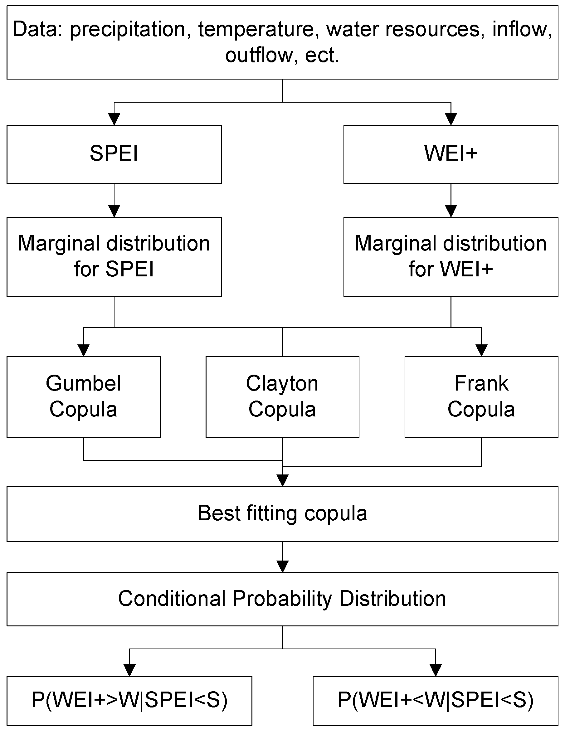
The whole copula-based process should flow the computational flow diagram shown in Figure 2.
3. Results and Discussion
3.1. SPEI Calculation Results
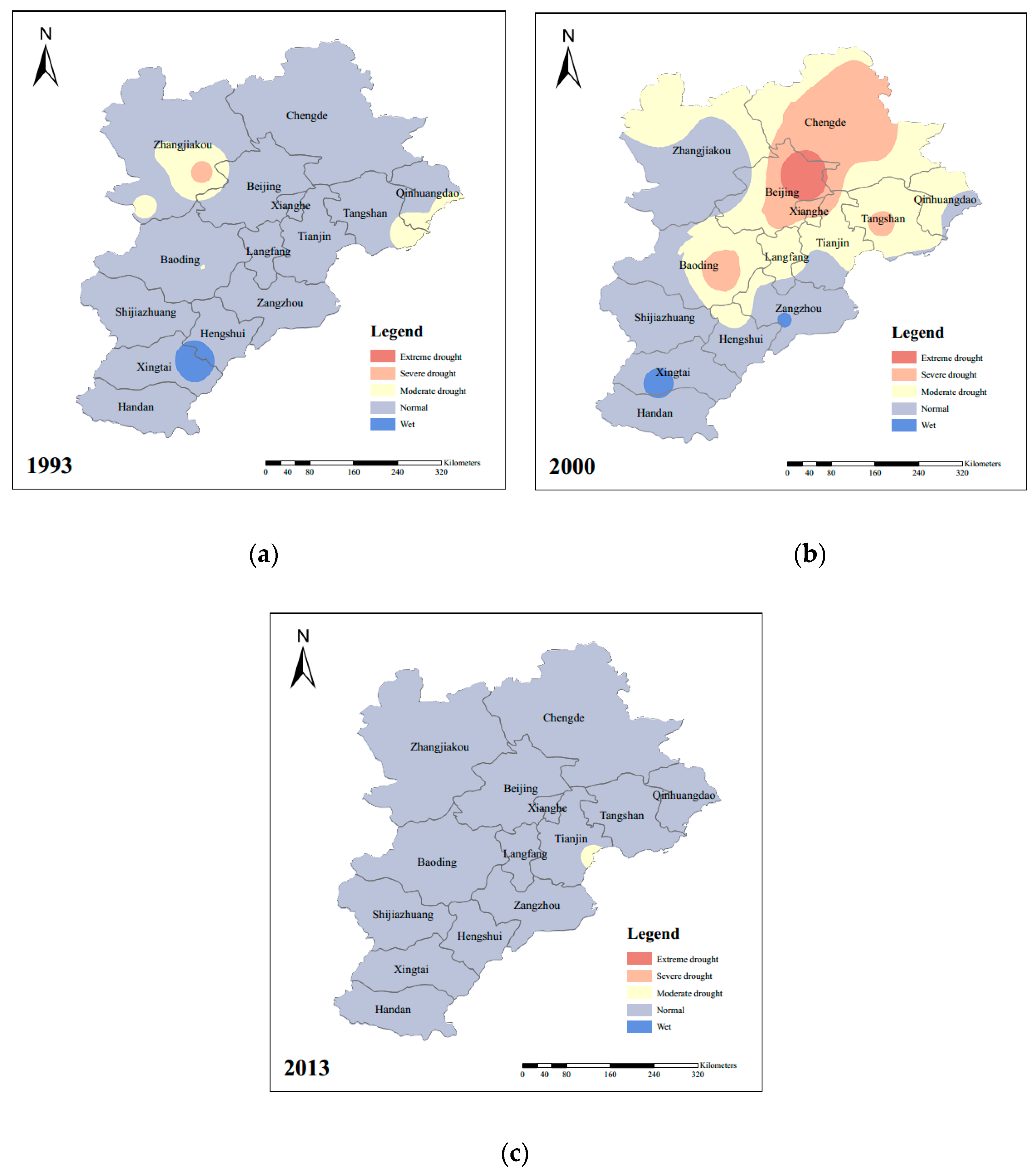
According to the calculation process of SPEI, the SPEI can be calculated at different time scales, which could be 3, 6, 12 or 24 months, for both seasonal and annual drought analysis. In this study, 12-month time scales (representing the drought situation of a whole year) of SPEI was selected, in order to share the same time scale with WEI+. The SPEIs calculated from each station were interpolated to the study domain using Inverse Distance Weighted method (IDW) and the three typical years (1993, 2000, 2013) of SPEI were shown in Figure 3. According to the classification of SPEI, five categories (Extreme drought, severe drought, moderate drought, normal, and wet) were used to illustrate the spatial distribution of drought. All three typical years showed different spatial distribution pattern. While the entire BTHMA was in normal wet condition in 2013 and most area of BTHMA was in normal wet condition in 1993, more than half of the BTHMA experienced a moderate to severe drought in 2000.
3.2. WEI+ Calculation Results
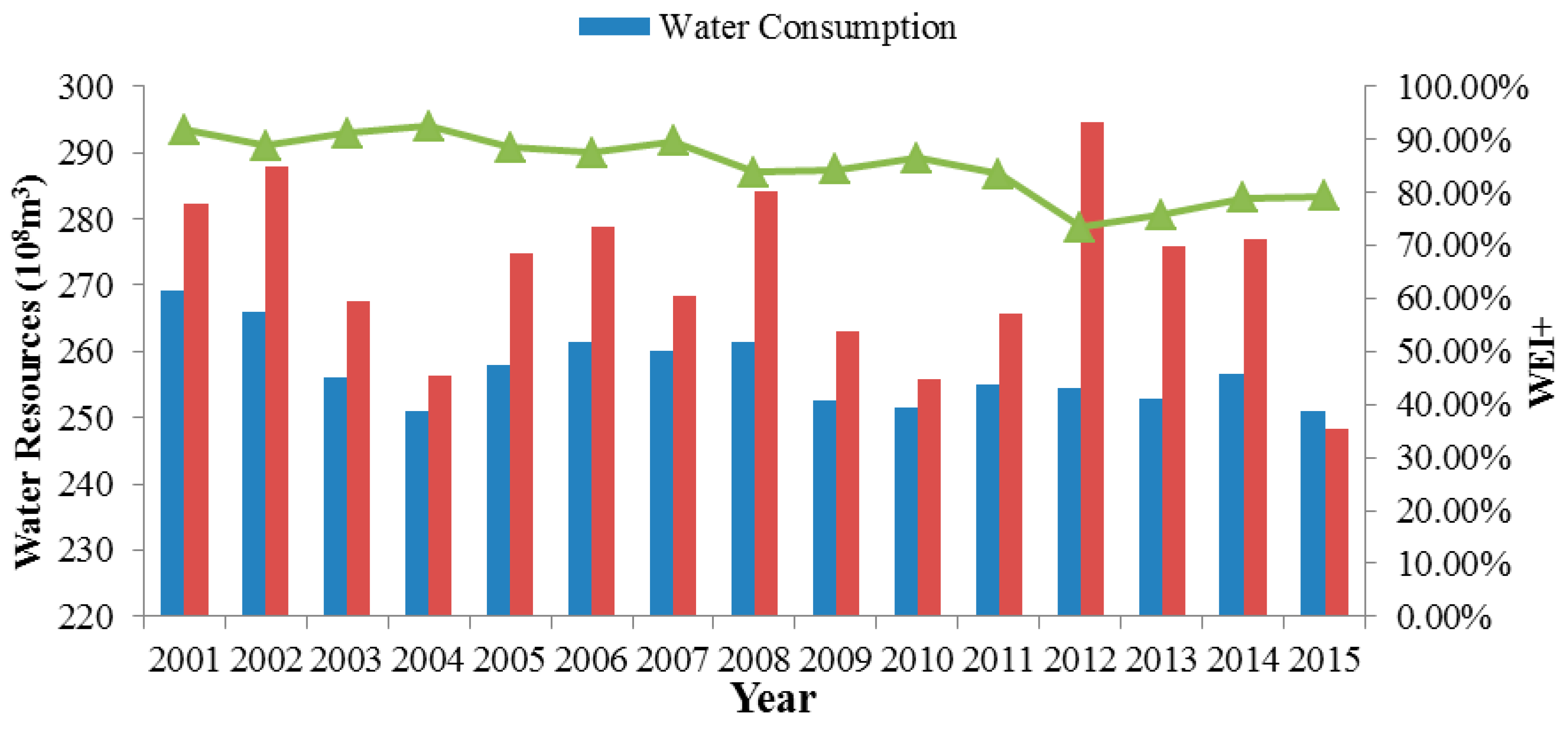
We used Equations (10) and (11) to calculate the renewable water resources given the intensive human activities from the large population in BTHMA. Based on the available data collected from Water Resources Bulletin, we use Equation (11) to calculate WEI+. The calculated WEI+ value of the entire study area from 2001 to 2015 is listed in Table 4 and Figure 4.
For every year except 2015, renewable water resources are larger than water consumption. During the study period, water consumption and renewable water resources do not show any changing pattern. They all fluctuate above and below their average values. During 2001 to 2015, the WEI+ values are all above 70%, higher surpass the threshold for water scarcity, indicating a serious situation of water scarcity. On the other hand, unlike the change of water consumption and renewable water resources, WEI+ showed a downward trend, which indicates that the water scarcity situation is getting better in recent years.
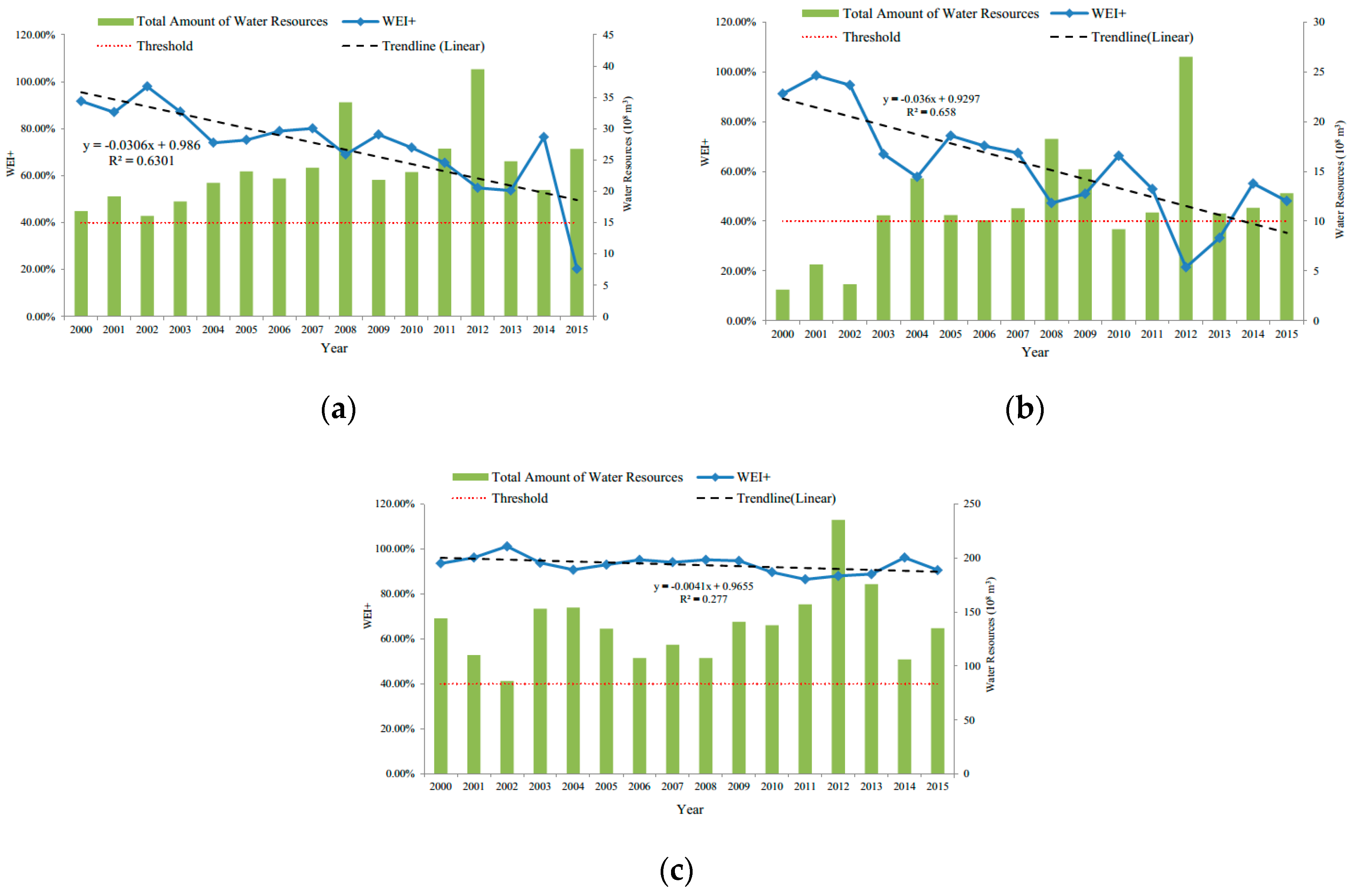
The WEI+ and total amount of water resources for Beijing, Tianjin, and Hebei are shown in Figure 5. The WEI+ values for most years in all three districts are above the threshold 40%, meaning that all three districts share the same problem of water scarcity. While the water scarcity situation of Beijing and Tianjin is moderating, the negative slopes of the WEI+ trend lines indicate a significant decline of water resources in the two districts especially Tianjin, the WEI+ value of 2012 and 2013 is below the threshold. As for Hebei Province, WEI+ stays very stable with an average value of 93.05%, much higher than the threshold 40%. In fact, Hebei Province is facing the most serious water scarcity problem, which has already influenced the local ecosystem. Over exploitation of groundwater in Hebei Province has already caused groundwater funnel and uneven settlement.
According to the Equations (7)–(11), the change of WEI+ value mainly related to three parameters, abstractions, returns, and outflows. For this study area, water consumption does not change a lot between years, so abstractions fluctuant over the long-term average value. Returns include wastewater reuse and rainwater, this number is increasing. In recent years, as water saving technique develops rapidly, the technology of sewage treatment and rainwater recovery is gradually maturing, much amount of this kind of water returns to the water supply system. These kinds of water can effectively relieve the regional water scarcity situation. The other item, outflows, is closely related to local water resources. When precipitation is adequate, the local water resources for the specific year are large, so the outflow is larger than other years, resulting in the smaller value of WEI+.
3.3. Conditional Probability Distribution between SPEI and WEI+
The WEI+ represented the spatial polygon data for the whole area, while the SPEI represented the spatial point data for specific meteorological station. When using copulas to establish the joint probability distribution, the SPEI and WEI+ data should share the same attribute, i.e., both polygon data or point data. So, the SPEI point data was interpolated into polygon data, using IDW ordinary Kriging interpolation method. After getting the SPEI polygon data, the value of SPEI for different region can be calculated, which should correspond to the WEI+ data.
The Kendall test was calculated to measure the statistical dependency between SPEI and WEI+. The Kendall’s τ between SPEI and WEI+ was 0.658, indicating a positive dependence between these two variables. So, copulas could be used to establish the joint distribution of them. In this study, the Gumbel, Frank, and Clayton copulas were applied to establish the joint distribution. The OLS, MSE, AIC and BIC criteria were used to compare the fits of the different copula models and to select the model that best described the dependency between SPEI and WEI+. The results, which were presented in Table 5, showed that the best-fitting model was the Gumbel copula; therefore, it was chosen for use in this study.
According to the mechanism of drought and water scarcity, meteorological drought may happen when natural precipitation is not enough for a certain period. When meteorological drought happens, and sustains a certain period, it may cause the deficient of water supply. When water supply cannot meet the need of water consumption for the society, then water scarcity may happen. Thus, meteorological drought is the precondition of water scarcity. When analysing the conditional probability, SPEI was set as the precondition. Two forms of conditional probability distribution were calculated according to Equations (20) and (21).
When SPEI is equal to or less than a threshold, i.e., SPEI ≤ s, the probability of WEI+ ≥ w can be calculated based on Equation (20). The results were shown in Figure 6. There were four curves in this diagram, illustrating SPEI ≤ 1, SPEI ≤ −1, SPEI ≤ −1.5, and SPEI ≤ −2, respectively. According to the classification of SPEI, SPEI ≥ 1 represents the situation of no drought happened. SPEI ≤ −1 represents the situation of moderately drought and worse. SPEI ≤ −1.5 represents the situation of severer drought and worse. SPEI ≤ −2 represents the situation of extreme drought and worse. The WEI+ represents the water exploitation stress on natural water system, so the larger the value of WEI+, the worse the water scarcity situation. From the four curves in Figure 6, we can see that the probability of WEI+ ≥ w is larger when the drought situation is severer. The probabilities of WEI+ ≥ w under different situations are listed in Table 6. When the drought situation is fixed, for example, SPEI ≤ −1.5, then the probability of WEI+ ≥ w becomes smaller as the threshold w gets larger. This phenomenon indicates that such extreme water scarcity situation, especially when WEI+ ≥ 0.9, is not likely to happen when drought situation does not reach to extreme drought. As for the same condition probability, the severer the drought situation, the larger the threshold w of WEI+. For example, when the condition probability is set as 0.6, under SPEI ≤ −1, the threshold w should be 0.81 (i.e., when SPEI ≤ −1, the probability of WEI+ ≥ 0.81 is 0.6). While under SPEI ≤ −2, the threshold w should be 0.95 (i.e., when SPEI ≤ −2, the probability of WEI+ ≥ 0.95 is 0.6).
When SPEI is equal to or less than a threshold, i.e., SPEI ≤ s, the probability of WEI+ ≤ w can be calculated based on Equation (21). The results were shown in Figure 7. There were four curves in this diagram, illustrating SPEI ≤ 1, SPEI ≤ −1, SPEI ≤ −1.5, and SPEI ≤ −2, respectively. Some laws of the curves can be observed from Figure 7. The probability of WEI+ ≤ w gets smaller as drought situation becomes severer. That’s easy to understand, because the curve of SPEI ≤ 1 contains other curves. Therefore, the curve of SPEI ≤ 1 is above all the other curves in the Figure. As for the fixed condition probability, when drought situation gets severer, the corresponding threshold w gets lager. This phenomenon indicates that severer drought may cause more serious water scarcity situation.
This copula-based conditional probability between SPEI and WEI+ not only reveals the occurrence of water scarcity in Beijing–Tianjin–Hebei Metropolitan Areas but also provides a probability distribution of water scarcity under different drought conditions. Because this conditional probability distribution is established based on calculated SPEI and WEI+ index, which can be regarded as historical data, it can represent the drought and water scarcity situations of the study area, thus can be used for future prediction. For example, if we know which kind of drought might happen in the future, we can use this conditional probability distribution to predict the probability of water scarcity in different level. This risk probability can provide technical support for government managers during policy making.
Copula functions are effective tools for establishing relationships between related variables based on a nonlinear approach. In this study, due to the limited data source related to water resources, we only obtained 15 annual data for WEI+ calculation. The limited data may to some extent reduce the reliability of the copula model. And the temporal pattern of drought and water scarcity within a year could not be estimated without the monthly water resources data in the future, if we get longer time series of data and monthly data, we might be able to establish a better conditional probability distribution, and better analyse the annual and inter-annual temporal patterns of drought and water scarcity, which should be more reliable for prediction. Moreover, this analysis method can also be used in other study areas. In addition, the WEI+ was barely used to evaluate water scarcity situation in China. The threshold of WEI+ in this study made reference to the studies of European countries. Further study should focus on the applicability of WEI+ in China and how to determine the threshold of WEI+ as well.
4. Conclusions
In this paper, copulas were applied to analyse the probabilistic relationship between meteorological drought (SPEI as indicator) and water scarcity (WEI+ as indicator) for two conditions (WEI+ ≥ w and WEI+ ≤ w) under SPEI ≤ s in Beijing–Tianjin–Hebei Metropolitan Areas in China. The spatial distribution of SPEI and WEI+ were also analysed.
From the results of spatial distribution, SPEI showed different spatial distribution patterns for each year. In general, the southern part of the study area was wetter than other parts. The middle part was drier, with moderate drought happened for most times. As for WEI+, Hebei Province had the largest WEI+ value (average 93.05%), while Tianjin had the smallest WEI+ value (average 62.36%), with Beijing in the middle (average 72.60%). The WEI+ of all three provinces (cities) was above the threshold 40%, indicating the water scarcity problem for all regions, among which Hebei Province suffered the most. From 2000 to 2015, WEI+ of Beijing and Tianjin showed an obvious downward trend, while Hebei did not. This indicated that water scarcity situation of Beijing and Tianjin has been alleviated in recent year, while Hebei still suffering it.
When establishing the copula functions, Gumbel copula was selected as the best-fitting copula between SPEI and WEI+. Based on the conditional probability method, the probability of water scarcity was calculated for two conditions (WEI+ ≥ w and WEI+ ≤ w). Under the same drought condition, the probability of extreme water scarcity (WEI+ ≥ w) decreased as the threshold w increased. When more serious drought happened, the probability of WEI+ ≥ w was larger, while the probability of WEI+ ≤ w was smaller, compared to less serous droughts. According to the conditional probability distribution, when drought happened (including moderate, severe and extreme drought), the probability of WEI+ ≥ 0.8 was around 0.6, the probability of WEI+ ≥ 1 was around 0.19. While under the same condition, the probability of WEI+ ≤ 0.8 was around 0.4, the probability of WEI+ ≤ 1 was around 0.81.
The method proposed in this study gives a water manager a tool to quantify the difference between drought and water scarcity, thus distinguish between natural and human effects on anomalies and adapt his/her management accordingly. This method could be used in other regions when facing the same situation. Then water resources managers could make decisions for adapting to the natural variability (drought) and combating water scarcity.
Author Contributions
Conceptualization, H.W.; Formal analysis, L.F.; Methodology, L.F.; Project administration, H.W.; Resources, H.W.; Supervision, Z.L.; Writing—original draft, L.F.; Writing—review and editing, Z.L. and N.L.
Funding
This research was supported by the National Natural Science Foundation of China (Grant number: 51479003 and 51879010), and the National Key R&D Program of China (Grant number: 2018YFC0407900-3 and 2017YFC1502701).
Acknowledgments
The authors would like to thank the constructive comments and suggestions from two anonymous reviewers and the editors.
Conflicts of Interest
The authors declare no conflict of interest.
References
- Pedro-Monzonís, M.; Solera, A.; Ferrer, J.; Estrela, T.; Paredes-Arquiola, J. A review of water scarcity and drought indexes in water resources planning and management. J. Hydrol. 2015, 527, 482–493. [Google Scholar] [CrossRef] [Green Version]
- Fan, L.; Wang, H.; Wang, C.; Lai, W.; Zhao, Y. Exploration of use of copulas in analysing the relationship between precipitation and meteorological drought in Beijing, China. Adv. Meteorol. 2017, 43, 1–11. [Google Scholar] [CrossRef]
- UN-WATER. Coping with Water Scarcity: A Strategic Issue and Priority for System-Wide Action. Available online: www.unwater.org/downloads/waterscarcity.pdf (accessed on 16 July 2012).
- FAO. Coping with Water Scarcity. Challenge of the Twenty-First Century. Available online: http://www.fao.org/nr/water/docs/escarcity.pdf (accessed on 1 March 2007).
- Van Loon, A.F.; Van Lanen, H.A.J. Making the distinction between water scarcity and drought using an observation-modeling framework. Water Resour. Res. 2013, 49, 1–20. [Google Scholar] [CrossRef]
- EU. Report on the Review of the European Water Scarcity and Droughts Policy, Communication from the Commission to the European Parliament and the Council, The European Economic and Social Committee and the Committee of the Regions. 2012. Available online: https://climate-adapt.eea.europa.eu/metadata/publications/report-on-the-review-of-the-european-water-scarcity-and-drought-policy/11309505 (accessed on 7 November 2018).
- Strosser, P.; Dworak, T.; Garzon, P.A.; Berglund, M.; Schmidt, G. Gap analysis of the Water Scarcity and Droughts Policy in the EU. Final report. European Commission Tender ENV.D.1/SER/2010/0049/Acteon 2012. Available online: http://ec.europa.eu/environment/water/quantity/pdf/WSDGapAnalysis.pdf (accessed on 7 November 2018).
- Mckee, T.B.; Doesken, N.J.; Kleist, J. The relationship of drought frequency and duration to time scales. In Proceedings of the 8th Conference on Applied Climatology, Anaheim, CA, USA, 17–22 January 1993; American Meteorological Society: Boston, MA, USA, 1993. [Google Scholar]
- Vicente-Serrano, S.M.; Beguería, S.; Lópezmoreno, J.I. A multi-scalar drought index sensitive to global warming: The standardized precipitation evapotranspiration index. J. Clim. 2010, 23, 1696–1718. [Google Scholar] [CrossRef]
- Palmer, W. Meteorological Drought. U.S. Department of Commerce Weather Bureau Research Paper. 1965. Available online: https://www.fws.gov/southwest/es/documents/R2ES/LitCited/LPC_2012/Palmer_1965.pdf (accessed on 7 November 2018).
- Faergemann, H. Update on Water Scarcity and Droughts Indicator Development; EC Expert Group on Water Scarcity & Droughts: Denmark, 2012. [Google Scholar]
- Falkenmark, M.; Widstrand, C. Population and water resources: A delicate balance. Potul. Bull. 1992, 47, 1–36. [Google Scholar]
- Estrela, T.; Vargas, E. Drought management plans in the European Union. The case of Spain. Water Resour. Manag. 2012, 26, 1537–1553. [Google Scholar] [CrossRef]
- Mortazavi, M.; Kuczera, G.; Cui, L. Multiobjective optimization of urban water resources: Moving toward more practical solutions. Water Resour. Res. 2012, 48, 3514. [Google Scholar] [CrossRef]
- Mazzanti, B.; Checcucci, G.; Monacelli, G.; Puma, F.; Vezzani, C. Drought and Water Scarcity Indicators: Experience and Operational Applications in Italian Basins. In Geophysical Research Abstracts; EGU General Assembly: Vienna, Austria, 2013; EGU2013-10311. [Google Scholar]
- Kossida, M.; Mimikou, M. An indicators’ based approach to Drought and Water Scarcity Risk Mapping in Pinios River Basin, Greece. In Geophysical Research Abstracts; EGU General Assembly: Vienna, Austria, 2013; EGU2013-6349, 2013. [Google Scholar]
- Van Lanen, H.A.J.; Tallaksen, L.M.; Stahl, K.; Van Loon, A.F.; Van Huijgevoort, M.H.J.; Corzo Perez, G.A. Drought, Water Scarcity and Climate Change. In Geophysical Research Abstracts; EGU General Assembly: Vienna, Austria, 2012; EGU2012-2143-2. [Google Scholar]
- Chen, F.; Li, J. Quantifying drought and water scarcity: A case study in the luanhe river basin. Nat. Hazards. 2016, 81, 1913–1927. [Google Scholar] [CrossRef]
- Cai, W.; Zhang, Y.; Chen, Q.; Yao, Y. Spatial patterns and temporal variability of drought in Beijing-Tianjin-Hebei metropolitan areas in China. Adv. Meteorol. 2015, 2015, 1–14. [Google Scholar] [CrossRef]
- Thornthwaite, C.W. An approach toward a rational classification of climate. Geogr. Rev. 1948, 38, 55–94. [Google Scholar] [CrossRef]
- Tan, C.; Yang, J.; Li, M. Temporal-spatial variation of drought indicated by SPI and SPEI in Ningxia hui autonomous region, china. Atmosphere 2015, 6, 1399–1421. [Google Scholar] [CrossRef]
- Raskin, P.; Gleick, P.; Kirshen, P.; Pontius, G.; Strzepek, K. Comprehensive Assessment of the Freshwater Resources of the World. Water Futures: Assessment of Long-Range Patterns and Problems; Stockholm Sweden Stockholm Environment Institute: Stockholm, Sweden, 1997. [Google Scholar]
- Lane, M.E.; Kirshen, P.H.; Vogel, R.M. Indicators of impacts of global climate change on US water resources. J. Water. Res. Plan. Mang. 1999, 125, 194–204. [Google Scholar] [CrossRef]
- Alcamo, J.; Thomas, H.T.; Rösch, T. World Water in 2025-Global Modeling Scenarios for the World Commission on Water for the 21st Century; Report A0002; Center for Environmental Systems Research: University of Kassel, Kassel, Germany, 2000. [Google Scholar]
- Sklar, A. N-Dimensional Distribution Functions and their Margins; L’Institut de statistique de l’universite de Paris: Paris, France, 1959; pp. 229–231. [Google Scholar]
- Nelsen, R.B. An Introduction to Copulas; Springer: New York, NY, USA, 2006. [Google Scholar]
- Qian, L.; Wang, H.; Dang, S.; Wang, C.; Jiao, Z.; Zhao, Y. Modelling bivariate extreme precipitation distribution for data-scarce regions using Gumbel-Hougaard copula with maximum entropy estimation. Hydrol. Process. 2017, 32. [Google Scholar] [CrossRef]
- Moazami, S.; Golian, S.; Kavianpour, M.R.; Hong, Y. Uncertainty analysis of bias from satellite rainfall estimates using copula method. Atmos. Res. 2014, 137, 145–166. [Google Scholar] [CrossRef]
- Jordanger, L.A.; Tjøstheim, D. Model selection of copulas: AIC versus a cross validation copula information criterion. Stat. Prpbabil. Lett. 2014, 92, 249–255. [Google Scholar] [CrossRef]
- Schwarz, G. Estimating the dimension of a model. Ann. Stat. 1978, 6, 15–18. [Google Scholar] [CrossRef]
- Brunner, M.I.; Favre, A.C.; Seibert, J. Bivariate return periods and their importance for flood peak and volume estimation. Wiley Interdiscip. Rev. Water 2016, 3, 819–833. [Google Scholar] [CrossRef]
- Stamatatou, N.; Vasiliades, L.; Loukas, A. Bivariate Flood Frequency Analysis Using Copulas. Proceedings 2018, 2, 635. [Google Scholar] [CrossRef]
- Azam, M.; Maeng, S.J.; Kim, H.S.; Murtazaev, A. Copula-Based Stochastic Simulation for Regional Drought Risk Assessment in South Korea. Water 2018, 10, 359. [Google Scholar] [CrossRef]
- Hesami Afshar, M.; Sorman, A.U.; Yilmaz, M.T. Conditional Copula-Based Spatial–Temporal Drought Characteristics Analysis—A Case Study over Turkey. Water 2016, 8, 426. [Google Scholar] [CrossRef]
- Yuan, F.; Ma, M.; Ren, L.; Shen, H.; Li, Y.; Jiang, S. Possible future climate change impacts on the hydrological drought events in the Weihe river basin, China. Adv. Meteorol. 2015, 2016, 1–14. [Google Scholar] [CrossRef]
- Shiau, J.T.; Modarres, R. Copula-based drought severity-duration-frequency analysis in Iran. Meteorol. Appl. 2009, 16, 481–489. [Google Scholar] [CrossRef] [Green Version]
Figure 1.
Sketch map of study area.

Figure 2.
The computational flow diagram.

Figure 3.
(a) Spatial distribution of SPEI in 1993; (b) Spatial distribution of SPEI in 2000; (c) Spatial distribution of SPEI in 2013.
Figure 3.
(a) Spatial distribution of SPEI in 1993; (b) Spatial distribution of SPEI in 2000; (c) Spatial distribution of SPEI in 2013.

Figure 4.
WEI+ of the whole study area from 2001 to 2015.

Figure 5.
(a) WEI+ of Beijing from 2001 to 2015; (b) WEI+ of Tianjin from 2001 to 2015; (c) WEI+ of Hebei Province from 2001 to 2015.
Figure 5.
(a) WEI+ of Beijing from 2001 to 2015; (b) WEI+ of Tianjin from 2001 to 2015; (c) WEI+ of Hebei Province from 2001 to 2015.

Figure 6.
Probability distributions of WEI+ ≥ w when SPEI ≤ s.

Figure 7.
Probability distributions of WEI+ ≤ w when SPEI ≤ s.


Table 1.
Differences between drought and water scarcity.
| Aspects | Drought | Water Scarcity |
|---|---|---|
| Causes | Natural, due to a deficient of precipitation over a certain time period. | Man-made, due to the increasing water consumption over natural renewable water resources. |
| Occurrence | Drought is a normal, recurrent feature of all climates and can happen anywhere. | Water scarcity usually happens in places where population is larger while natural water resources are not enough. |
| Timescale | Drought can last from a few weeks to several years. | Usually, water scarcity may cause permanent damage to water ecosystems. |
| Impacts | The impacts cause by drought may be variable, according to its duration, severity, and also the vulnerability of society. It is more likely to influence the natural water cycle. | The impacts cause by water scarcity is more social. It will directly influence agricultural, industrial and domestic water consumption. |
| Spatial distribution | Usually evaluated by river basins, and can happen in both small and large scales. | Usually evaluated by administrative regions, and can happen in both small and large scales. |
| Interaction | When droughts occur in an area characterized by water scarcity, their impact will be more severe, as they are more vulnerable. Heat waves can aggravate droughts and water scarcity situations. Water scarcity can also be an effect of overexploitation due to (concurrent) drought events, but this does not apply vice versa (drought is not an effect of water scarcity) | |
| Risk | The risk of drought depends on the hazard, and the vulnerability and exposure of hazard-affected bodies. | The risk of water scarcity not only depends on the hazard, the vulnerability and exposure of hazard-affected bodies, but also depends on the reliability and resistance of hazard-affected bodies. The vulnerability and exposure may increase the risk, while the reliability and resistance can decrease the risk. |
| Indicators | SPI [8], SPEI [9], Palmer Index [10] | WEI+ [11], the Falkenmark indicator [12] |
Table 2.
Basic information of meteorological stations.
| Station Name | Latitude (N) | Longitude (E) | Duration |
|---|---|---|---|
| Beijing | 39.80 | 116.47 | January 1951—December 2015 |
| Tianjin | 39.08 | 117.07 | January 1954—December 2015 |
| Tanggu | 39.05 | 117.72 | January 1954—December 2015 |
| Bohai | 38.45 | 118.42 | January 2004—December 2015 |
| Shijiazhuang | 38.03 | 114.42 | January 1955—December 2015 |
| Baoding | 38.85 | 115.52 | January 1955—December 2015 |
| Chengde | 40.98 | 117.95 | January 1951—December 2015 |
| Langfang | 39.12 | 116.38 | January 1957—December 2015 |
| Qinhuangdao | 39.85 | 119.52 | January 1954—December 2015 |
| Tangshan | 39.67 | 118.15 | January 1957—December 2015 |
| Xingtai | 37.07 | 114.50 | January 1954—December 2015 |
| Zhangjiakou | 40.78 | 114.88 | January 1956—December 2015 |
| Botou | 38.08 | 116.55 | January 1996—December 2015 |
| Huailai | 40.40 | 115.5 | January 1954—December 2015 |
| Huanghua | 38.37 | 117.35 | January 1960—December 2015 |
| Laoting | 39.43 | 118.88 | January 1957—December 2015 |
| Miyun | 40.38 | 116.87 | January 1989—December 2015 |
| Nangong | 37.37 | 115.38 | January 1958—December 2015 |
| Qinglong | 40.40 | 118.95 | January 1957—December 2015 |
| Raoyang | 38.23 | 115.73 | January 1957—December 2015 |
| Weichang | 41.93 | 117.75 | January 1951—December 2015 |
| Weixian | 39.83 | 114.57 | January 1954—December 2015 |
| Zhangbei | 41.15 | 114.70 | January 1956—December 2015 |
| Zunhua | 40.20 | 117.95 | January 1956—December 2015 |
Table 3.
Classification of Standard Precipitation and Evapotranspiration Index (SPEI) values.
| Class | SPEI Value | Description | Class | SPEI value | Description |
|---|---|---|---|---|---|
| 1 | SPEI ≥ 2.00 | Extremely wet | 5 | −1.50 ≤ SPEI < −1.00 | Moderate drought |
| 2 | 1.50 ≤ SPEI < 2.00 | Very wet | 6 | −2.00 ≤ SPEI < −1.50 | Severe drought |
| 3 | 1.00 ≤ SPEI < 1.50 | Moderately wet | 7 | SPEI < −2.00 | Extreme drought |
| 4 | −1.00 ≤ SPEI < 1.00 | Near normal |
Table 4.
The calculated water exploitation index plus (WEI+) value from 2001 to 2015.
| Year | Water Consumption (×108 m3) | RWR (×108 m3) | WEI+ |
|---|---|---|---|
| 2001 | 269.31 | 282.41 | 91.83% |
| 2002 | 265.97 | 287.90 | 88.87% |
| 2003 | 256.15 | 267.64 | 91.20% |
| 2004 | 250.97 | 256.45 | 92.44% |
| 2005 | 258.07 | 274.76 | 88.42% |
| 2006 | 261.30 | 278.80 | 87.55% |
| 2007 | 260.00 | 268.31 | 89.65% |
| 2008 | 261.47 | 284.25 | 83.85% |
| 2009 | 252.59 | 262.99 | 84.23% |
| 2010 | 251.59 | 255.69 | 86.42% |
| 2011 | 255.07 | 265.67 | 83.52% |
| 2012 | 254.36 | 294.70 | 73.40% |
| 2013 | 252.86 | 275.90 | 75.70% |
| 2014 | 256.49 | 277.05 | 79.01% |
| 2015 | 251.08 | 248.37 | 79.21% |
Table 5.
Parameter estimation and criteria results of copula fitting.
| Items | Gumbel | Frank | Clayton |
|---|---|---|---|
| Parameter estimation θ | 1.5905 | 3.7628 | 0.7679 |
| OLS | 0.0245 | 0.0250 | 0.1065 |
| MSE | 0.0006 | 0.00062 | 0.0114 |
| AIC | −361.55 | −359.65 | −217.45 |
| BIC | −356.92 | −355.02 | −212.82 |
Table 6.
The probability of WEI+≥w under different drought conditions.
| Water Scarcity Situation | SPEI ≤ −1 | SPEI ≤ −1.5 | SPEI ≤ −2 | SPEI ≤ 1 |
|---|---|---|---|---|
| WEI+ ≥ 0.5 | 97.76% | 98.80% | 99.41% | 91.89% |
| WEI+ ≥ 0.6 | 94.53% | 97.03% | 98.54% | 82.77% |
| WEI+ ≥ 0.7 | 85.25% | 91.80% | 95.93% | 63.27% |
| WEI+ ≥ 0.8 | 60.22% | 75.79% | 87.63% | 32.28% |
| WEI+ ≥ 0.9 | 27.40% | 45.52% | 68.47% | 10.89% |
© 2018 by the authors. Licensee MDPI, Basel, Switzerland. This article is an open access article distributed under the terms and conditions of the Creative Commons Attribution (CC BY) license (http://creativecommons.org/licenses/by/4.0/).
Share and Cite
MDPI and ACS Style
Fan, L.; Wang, H.; Liu, Z.; Li, N. Quantifying the Relationship between Drought and Water Scarcity Using Copulas: Case Study of Beijing–Tianjin–Hebei Metropolitan Areas in China. Water 2018, 10, 1622. https://doi.org/10.3390/w10111622
AMA Style
Fan L, Wang H, Liu Z, Li N. Quantifying the Relationship between Drought and Water Scarcity Using Copulas: Case Study of Beijing–Tianjin–Hebei Metropolitan Areas in China. Water. 2018; 10(11):1622. https://doi.org/10.3390/w10111622
Chicago/Turabian StyleFan, Linlin, Hongrui Wang, Zhiping Liu, and Na Li. 2018. "Quantifying the Relationship between Drought and Water Scarcity Using Copulas: Case Study of Beijing–Tianjin–Hebei Metropolitan Areas in China" Water 10, no. 11: 1622. https://doi.org/10.3390/w10111622
Note that from the first issue of 2016, this journal uses article numbers instead of page numbers. See further details here.