Spatiotemporal Variations in Mercury Bioaccumulation at Fine and Broad Scales for Two Freshwater Sport Fishes

Abstract

Bioaccumulation of mercury in sport fish is a complex process that varies in space and time. Both large-scale climatic as well as fine-scale environmental factors are drivers of these space-time variations. In this study, we avail a long-running monitoring program from Ontario, Canada to better understand spatiotemporal variations in fish mercury bioaccumulation at two distinct scales. Focusing on two common large-bodied sport fishes (Walleye and Northern Pike), the data were analyzed at fine- and broad-scales, where fine-scale implies variations in bioaccumulation at waterbody- and year-level and broad-scale captures variations across 3 latitudinal zones (~5° each) and eight time periods (~5-year each). A series of linear mixed-effects models (LMEMs) were employed to capture the spatial, temporal and spatiotemporal variations in mercury bioaccumulation. Fine-scale models were overall better fit than broad-scale models suggesting environmental factors operating at the waterbody-level and annual climatic conditions matter most. Moreover, for both scales, the space time interaction explained most of the variation. The random slopes from the best-fitting broad-scale model were used to define a bioaccumulation index that captures trends within a climate change context. The broad-scale trends suggests of multiple and potentially conflicting climate-driven mechanisms. Interestingly, broad-scale temporal trends showed contrasting bioaccumulation patterns—increasing in Northern Pike and decreasing in Walleye, thus suggesting species-specific ecological differences also matter. Overall, by taking a scale-specific approach, the study highlights the overwhelming influence of fine-scale variations and their interactions on mercury bioaccumulation; while at broad-scale the mercury bioaccumulation trends are summarized within a climate change context.

1. Introduction

Mercury pollution captured global attention during the tragic Minamata poisoning in Japan, which highlighted the fatal neurotoxic effects of consuming mercury tainted fish [1,2]. Canada has its own ongoing mercury tragedy in Grassy Narrows and areas downstream of a Dryden pulp and paper Mill, where more than 9000 kg of mercury were released into the English-Wabigoon River between 1963 and 1970. First Nations communities downstream were affected when they unknowingly ate mercury contaminated fish and multiple generations have suffered the neurotoxic, social and economic consequences that decimated a once thriving First Nation’s fishing and tourism economy [3]. Despite concerted global efforts to reduce mercury emissions, mercury as an anthropogenic pollutant remains a matter of grave concern, especially given that elemental mercury is highly mobile and often ends up in aquatic and terrestrial ecosystems far from the emission source [4,5,6,7]. In aquatic ecosystems the impact of mercury pollution is mainly associated with organic methylmercury (MeHg) [4,5]. MeHg is particularly detrimental as it can bioaccumulate and biomagnify such that older large-sized fishes at the apex of aquatic food chains have disproportionately higher amounts of mercury [4,5,8,9,10,11,12,13,14]. Thus, large-bodied fishes at the top of food chains are good indicators of mercury levels and when consumed by humans can have adverse long-term effects on human health and well-being [8,9,10,11,12]. In addition to the adverse impact on human health, mercury pollution has detrimental effects on wildlife, especially large predatory birds and mammals at the apex of food chains [15].

Both the United States and Canada have established monitoring programs at state and provincial levels to study fish mercury dynamics. Analyses of these large-scale databases typically show a declining trend in fish mercury levels between 1970 and 2000 [8,9,10]. However, there is substantial geographic variation in these long-term trends [8,9,11]. Most importantly, many regions are experiencing increasing mercury levels in several key sport fishes in recent years and this may have severe implications for human health if the trend continues [10,12]. Climate change, particularly the warming climatic conditions experienced by lakes in temperate regions is thought to be one of the likely reasons for the recent surge in mercury levels [10,12,13]. This is not surprising as climate is recognized as one of the key drivers of broad-scale variation in methylmercury concentration within aquatic systems [12,13]. However, the eventual effect of changing climate on fish mercury levels is a complex multi-scale process, which remains poorly understood to date. At the relatively fine scale of lake and watershed levels, warming conditions are known to increase net methylation rates and thus increase the overall amount of bioavailable methylmercury in a lake [16,17]. Warmer temperatures also affect mercury levels within waterbodies, by altering trophic position, food-chain length and productivity [18,19]. However, these community-level impacts are highly variable and are contingent on the species of fish and species composition [17]. Besides temperature, precipitation also impacts mercury availability in aquatic systems, especially via wet atmospheric deposition and surface run-offs [14,20]. Overall, broad-scale climatic conditions and fine-scale environmental factors at the waterbody and watershed scale together determine the amount of bioavailable MeHg, thus setting the exposure baseline for fishes.

The amount of mercury in a fish is eventually determined by consumption of mercury contaminated food. The final amount retained by an individual fish is a complex function of consumption, growth and metabolism. Fish with better growth efficiency (i.e., ratio of growth rate to consumption rate) tend to accumulate less mercury, while increased metabolism may demand higher rates of consumption thus increasing accumulation of mercury [14,21,22]. Fast growing fish with greater growth efficiency are hypothesized to accumulate less mercury since the net amount of biomass added is much greater for every unit of mercury gained, and this is referred to as growth dilution. Studies suggest that growth dilution is most likely in situations where fast growth rate is accompanied by low metabolic costs or high quality food (low in mercury contamination) [21,22]. In this context, rising temperatures are expected to increase fish growth rates and lead to growth dilution assuming metabolic costs remain below species threshold levels. These processes could potentially reduce overall fish mercury levels. In different circumstances, warmer temperatures may increase metabolic costs offsetting any reduction in fish mercury levels achieved via increased growth rates. And as mentioned earlier, a warming climate can also affect fish mercury levels by altering the amount of MeHg generated within waterbodies. Put together, climate as a broad-scale driver can directly and indirectly affect fish mercury bioaccumulation.

Studies also show a high degree of variation in fish mercury levels at the lake/waterbody scale independent of climate [23,24]. This fine-scale variation in fish mercury levels is attributed to drivers operating at the waterbody-level such as prey quality, competition, activity in the sediment microbial community and water chemistry variability as these factors are known to influence both the amount of bioavailable MeHg as well as fish growth and metabolism. However, very few studies take into consideration large-scale variation in MeHg availability or fish growth rates at the waterbody-scale in the context of mercury bioaccumulation, since data on both MeHg content in sediments and fish age are scarce.

In this study, we make use of a long running fish mercury monitoring program spanning 15 latitudinal degrees and 45 years (see Section 2) to characterize spatiotemporal variations in mercury bioaccumulation for two common freshwater sport fishes at two distinct scales. We also make use of the Ontario Ministry of Natural Resources and Forestry (OMNRF), Broadscale Monitoring (BSM) Program database, by combining fish mercury data from the Ontario Ministry of Environment, Conservation and Parks (OMECP) with fish age data from the Provincial BSM database for the first time. Using the full range of variation in fish size and mercury concentration, a series of mixed-effects models were used to capture: (i) fine-scale variations in mercury bioaccumulation at the individual waterbody- and year-level and (ii) broad-scale variation across three latitudinal zones (~5 decimal degrees each) and eight time periods (~5-year each). The broad-scale variation in fish mercury bioaccumulation were used to define a bioaccumulation index that summarizes mercury trends in space and time. We then explore the broad-scale spatiotemporal trends in mercury bioaccumulation within a climate change context. The BSM database has a comparable spatial scope and resolution to the contaminants database but focuses on ecosystem assessment of the health of fisheries and related taxa and includes fish age information rather than contaminants. The BSM program monitors lake ecosystems using a random sampling approach stratified by fisheries management zones. Using the linked databases, we evaluate fine-scale (i.e., waterbody-level) variation in fish growth rates for each species and we assess if there is any discernible latitudinal trend in the growth rate estimates. We then make use of the quantified growth rate variation at the waterbody level and the derived latitudinal trends to address the mercury bioaccumulation patterns.

2. Methods

2.1. Fish Mercury Data

We used one of the world’s largest known fish monitoring databases compiled by the OMECP, in partnership with OMNRF, to track pollutant loads in several key sport fishes. Department of Fisheries and Oceans at the Canada Centre of Inland Waters also conduct limited monitoring of fish mercury in Ontario inland waterbodies. But to keep the dataset consistent, we focused on extensive monitoring data collected by Government of Ontario. The Ontario-wide monitoring program began in 1970, that is, a temporal scope of more than 45 years (1970 onwards) and covers a broad climatic range with a latitudinal breadth of nearly 15 degrees (41.5° to 56.5°). Each data record provides fish species identity, length, body mass, sex and amount of mercury alongside information on lake or waterbody identity/name and geo-coordinates of the location where the fish was sampled. With multiple fish samples often taken at a given time and location and a total of 126,652 records from nearly 2700 lakes, the database provides a comprehensive picture of fish mercury levels and several key fish-level attributes.

2.2. Data Selection & Focal Species

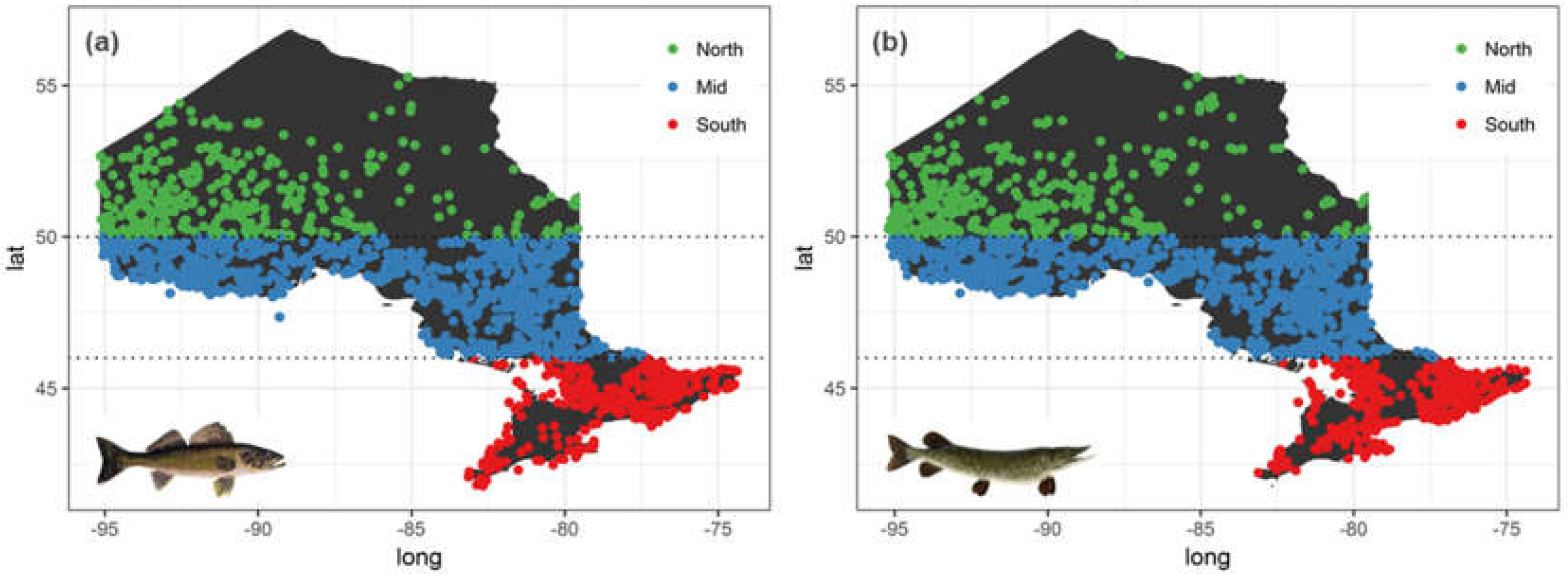
In order to develop a bioaccumulation index that captures variation in mercury levels across a broad range of climatic conditions, we chose species with the most widespread distribution across Ontario. Walleye (Sander vitreus) and Northern Pike (Esox lucius) were the best candidate species in this respect; their broad nearly identical distribution patterns that span most of Ontario (Figure 1).

Walleye is a native cool-water predatory fish that is common in most lakes of Canada and northern United States. Walleye, like many shoaling fishes, prefers large open waters and its large eyes enable it to hunt effectively in low light conditions, particularly at dusk and at night [25]. Northern Pike is an equally common cool-water predatory fish with a broad pan-artic distribution that includes Europe, Russia, Canada and northern United States. Unlike Walleye, Northern Pike is a large ambush predator that prefers to hunt during the day and like most ambush predators they need cover in the form of dense vegetation or submerged logs [26]. Also notable is the difference in body size with Walleye typically being smaller in size than Northern Pike. In Ontario, Northern Pike are known to attain an average size of 45–75 cm, whereas Walleye typically range between 35–58 cm. Walleye and Northern Pike are consumers at the top of aquatic food-chains that co-occur in several lakes and freshwater bodies in Ontario, however their ecology, feeding habits and growth differ substantially, making this pair of sport fishes particularly interesting to detect species-specific differences in mercury bioaccumulation. In a final data selection process, fish samples collected during the first 5 years (i.e., 1970–1974) were not included as they were selectively collected from locations within close proximity to known sources of mercury pollution and hence had disproportionately higher mercury levels. In summary, records between 1975 and 2015 of Walleye and Northern Pike were analyzed to develop the bioaccumulation index.

2.3. Mercury Bioaccumulation at Fine & Broad Scales

We analyzed fish mercury-body size relationships based on all possible combinations of spatial and temporal categories at two distinct scales. In other words, spatial, temporal and spatiotemporal variations in fish mercury bioaccumulation were analyzed first at a fine scale and later at a broad-scale resolution. For the fine-scale analysis, each individual waterbody and year were identified as spatial and temporal categories, respectively. This included a broad range of lakes and waterbodies, varying in both size (0.5 km² to 900 km²) and depth (1 m to 213 m). Whereas for the broad-scale analysis, the data for each species were divided into 8 temporal periods (1975–1979, 1980–1984, 1985–1990, 1990–1994, 1995–1999, 2000–2004, 2005–2009, 2010–2015) and 3 latitudinal zones (south: 40° N—46° N, mid: 46° N—50° N and north: >50° N). It is important to note that in addition to climate, the broadly defined latitudinal zones differ in lake sediment mercury levels such that north and mid zones are estimated to have greater loads of sedimental mercury relative to south zone [27]. Thus, in the broad-scale approach temporal categories were 5-year periods (except for the ‘2010–2015’ period) and spatial categories are 5°-wide latitudinal zones. The rationale behind analyzing mercury bioaccumulation at both fine and broad scales were twofold: (i) the fine-scale analyses captures the importance of lake-level limnological factors and annual climatic variations affecting mercury bioaccumulation, (ii) but given the haphazard nature of lake sampling through time (with very few lakes sampled consistently during the entire 41-year time period), a broad-scale approach was necessary wherein sparser data was grouped based on latitudinal zones and temporal periods. Such a broad-scale approach not only captures patterns in fish mercury at larger spatio-temporal scales but also effectively summarizes the more complex and intractable ecological variation that arises from processes operating at finer scales (i.e., the waterbody scale in our study) [28].

Mercury levels in fish typically follow an allometric relationship with body size [29]:

$$Z=a{X}^b$$

(1)

where $Z$ is the amount of mercury $\left(\mathsf{\mu }\mathrm{g}/\mathrm{g}\right)$, $X$ is fish body length (cm), a is a proportionality constant and b is a scaling exponent. When log-transformed, the allometric relationship takes the form of a linear model (shown below; Equation (2)), which was used in all the analyses.

$$\log \left(Z\right)=\log \left(a\right)+b\times \log \left(X\right)\Rightarrow \log \left(Z\right)={\beta }_0+{\beta }_1\log \left(X\right)$$

(2)

However, there is substantial variability in mercury sampling in both space and time. Out of the 2948 Walleye lakes sampled during the 41-year period, 43 lakes were sampled only once while the average sample size per lake was 16. Similarly, 88 lakes out of 2642 lakes were sampled only once in the 41-year period for Northern Pike, with an overall average of 12 samples per lake. In order to account for the uneven sampling in space and time, we used linear mixed-effects modeling (LMEM) approach. Mixed-effects models are ideal for such unbalanced data since group-level parameters are estimated by partial-pooling of data from other groups that make up the database [30,31]. In other words, partial pooling ensures that parameter estimates for a poorly sampled group ‘shrinks’ towards the global estimate by borrowing parameter estimates from well-sampled groups [31,32]. Hence, we used the above log-linear model (2) within a linear mixed-effects modeling framework with the spatial and temporal categories (as defined in previous paragraph) as crossed random effects of both intercepts and slopes to quantify the effect of space, time and space-time interactions [30]. At the fine scale of analysis, spatial effects are captured by individual waterbodies (WB) as random (grouping) factor, temporal effects are captured by treating each year (YR) as random factor and spatiotemporal interaction effects are captured by treating all unique waterbody-year combination (WB:YR) as a random factor. And at the broad scale, spatial effects are captured by considering each latitudinal zone (LZ) as a random grouping factor, temporal effects are captured by incorporating time period (TP) as the random factor and spatiotemporal interaction effects are captured by treating all latitudinal zone-time period combination (LZ:TP) as the random grouping factor. Put together, the mixed-models return random slope estimates, which are essentially size-standardized measures of mercury bioaccumulation for that spatial (lake or latitudinal zone), temporal category (year or 5-year period) or spatiotemporal category. In total, four distinct LMEM’s were separately fit at each scale of analyses for each species (i.e., Walleye and Northern Pike) to capture species-specific variations in mercury bioaccumulation at a given scale (

Table 1. Description of the LMEM’s used to capture spatial, temporal and spatiotemporal variation in mercury bioaccumulation at two distinct scales of analyses for Walleye and Northern Pike. Both response (Z, mercury concentration) and fixed-effect covariate (X, fish length) are log-transformed throughout but is not shown explicitly in the model formulae.

Scale of Analysis	Linear Mixed-Effect Models	Model Formula
Fine scale	Spatial effects	$Z_{iw}$ = ${\beta }_0$ + $W{B}_{0w}$ + (${\beta }_1$ + $W{B}_{1w}$) $X_i$ + ${\epsilon }_{il}$
	Temporal effects	$Z_{iy}$ = ${\beta }_0$ + $Y{R}_{0y}$ + (${\beta }_1$ + $Y{R}_{1y}$) $X_i$ + ${\epsilon }_{iy}$
	Spatial & temporal effects	$Z_{iwy}$ = ${\beta }_0$ + $W{B}_{0w}$ + (${\beta }_1$ + $W{B}_{1w}$) $X_i$ + $Y{R}_{0y}$ + (${\beta }_1$ + $Y{R}_{1y}$) $X_i$ + ${\epsilon }_{iwy}$
	Full model (spatial, temporal, & spatiotemporal interaction effects)	$Z_{iwy}$ = ${\beta }_0$ + $W{B}_{0w}$ + (${\beta }_1$ + $W{B}_{1w}$) $X_i$ + $Y{R}_{0y}$ + (${\beta }_1$ + $Y{R}_{1y}$) $X_i$ + $W{B}_{0w}\ast Y{R}_{0y}+({\beta }_1+W{B}_{1w})X_i\ast ({\beta }_1+Y{R}_{1y})X_i+{\epsilon }_{iwy}$
Broad scale	Spatial effects	$Z_{il}$ = ${\beta }_0$+ $L{Z}_{0l}$ + (${\beta }_1$ + $L{Z}_{1l}$) $X_i$ + ${\epsilon }_{il}$
	Temporal effects	$Z_{it}$ = ${\beta }_0$+ $T{P}_{0t}$ + (${\beta }_1$ + $T{P}_{1t}$) $X_i$ + ${\epsilon }_{it}$
	Spatial & temporal effects	$Z_{ilt}$ = ${\beta }_0$+ $L{Z}_{0l}$ + (${\beta }_1$ + $L{Z}_{1l}$) $X_i$ + $T{P}_{0t}$ + (${\beta }_1$ + $T{P}_{1t}$) $X_i+{\epsilon }_{ilt}$
	Full model (spatial, temporal, & spatiotemporal interaction effects)	$Z_{ilt}$ = ${\beta }_0$+ $L{Z}_{0l}$ + (${\beta }_1$ + $L{Z}_{1l}$) $X_i$ + $T{P}_{0t}$ + (${\beta }_1$ + $T{P}_{1t}$) $X_i$ $+L{Z}_{0l}\ast T{P}_{0t}+({\beta }_1+L{Z}_{1l})X_i\ast ({\beta }_1+T{P}_{1t})X_i+{\epsilon }_{ilt}$

Abbreviations: $Z_{iw}$ = mercury concentration in fish, i, collected from waterbody, w; $Z_{iy}$ = mercury concentration in fish, i, collected in year, y; $Z_{iwy}$ = mercury concentration in fish, i, collected from waterbody, w, during the year, y; $Z_{il}$ = mercury concentration in fish, i, collected from latitudinal zone, l; $Z_{it}$ = mercury concentration in fish, i, collected during time period, t; $Z_{ilt}$ = mercury concentration in fish, i, collected from latitudinal zone, l, during time period, t; $X_i$ = length of fish, i, ${\beta }_0$ = overall model intercept; ${\beta }_1=overalllmodelslope;$ $W{B}_{0w}=$ waterbody intercepts; $W{B}_{1w}=\mathrm{waterbody}\mathrm{slopes};$ $Y{R}_{0y}$ = year intercepts; $Y{R}_{1y}$ = year slopes; $L{Z}_{0l}$ = latitudinal zone intercepts; $L{Z}_{1l}$ = latitudinal zone slopes; $T{P}_{0t}$ $=\mathrm{time}\mathrm{period}\mathrm{intercepts};T{P}_{1t}$ = time period slopes; $\epsilon$ = residual term of the respective models. See Section 2 for more details on how latitudinal zones and time periods are defined.

).

Finally, for each species and scale the best mixed-effects model was identified using the information theoretic method—Akaike Information Criterion (AIC), where lower AIC values imply better model fit. And for the best model identified, the amount of variance accounted by each random factor was noted. All LMEMs were fit using lme4 package [33] and further analyzed with merTools package [34] in R [35].

For the broad-scale analysis, the best fit model was further evaluated to capture mercury bioaccumulation trends in space and time. To do so, the random slope coefficients from the best-fitting broad-scale model was compiled together to form a ‘bioaccumulation index’ based on all the random-effect groups involved. In summary, for each fish species the bioaccumulation index derived from the best-fitting LMEM at the broad-scale describes variation in the magnitude of mercury bioaccumulation across either latitudinal zones, temporal periods, or a combination of latitudinal zones and temporal periods. Overall, the broad-scale bioaccumulation index summarizes variations operating at finer-scales (at waterbody and annual space-time scales) across larger areas and longer time periods, such that the resulting bioaccumulation trends in space and time can be explored further in the context of changing climate conditions.

2.4. Summarizing 45 Years of Climate Change

To provide a climatic context for the broad-scale bioaccumulation trends, climatic conditions in Ontario were summarized for 45 years (1970–2015) using temperature, growing degree-days and precipitation measures because we were interested in understanding how climatic conditions can potentially influence fish mercury bioaccumulation at broad-scales. The climate data were sourced from Environment Canada’s historical climate data website (http://climate.weather.gc.ca/index_e.html). The website provides climate information for each station at daily, monthly and annual intervals. In line with the broad-scale analysis of mercury bioaccumulation trends, climate trends were captured across 5-year periods for each of the three latitudinal zones. A total of 9 temporal periods were examined, with the earliest being 1970–1975 and ending at 2010–2015. Within each latitudinal zone, stations with complete climate data were used to characterize the climate trends. However, for many stations complete climate data spanning the entire 45-year period were not available, which resulted in the selection of very few compatible stations. Thus, three weather stations each were selected for south (Trenton, Ottawa and Glasgow) and mid (Chalk, Sudbury and Kenora) latitudinal zones, whereas in the north, only two weather stations were available (Sioux and Moosonee). In summary, average daily temperature and precipitation were estimated for each 5-year period and latitudinal zones, whereas number of growing degree days were estimated as the cumulative number of days when average daily temperature was above 5 °C.

2.5. Variation in Fish Growth Rate at Waterbody-Level

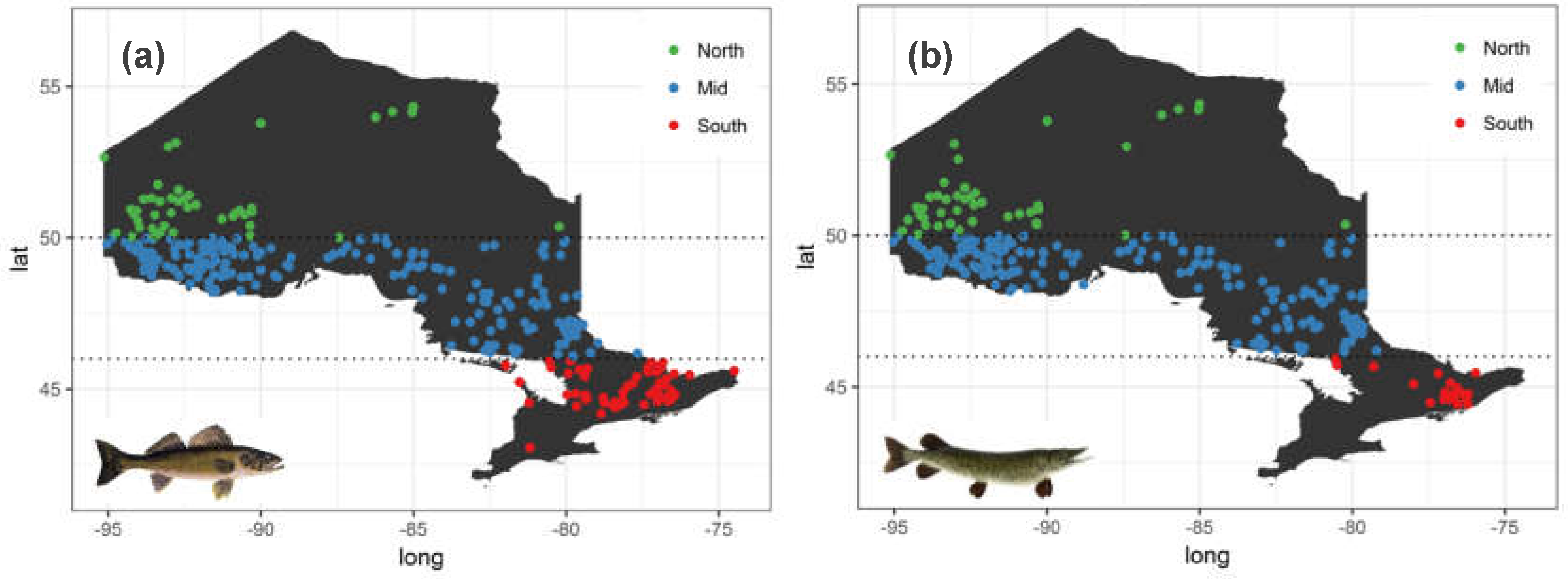
Besides climate, fish-level factors, particularly fish growth rate variation at the waterbody-scale can explain the observed fine-scale mercury bioaccumulation patterns. Variation among waterbodies in abiotic and biotic conditions leads to variation in fish growth rates at the waterbody-level and this fine-scale variation in growth rate is one of the key drivers (besides variation in the amount of bio-available methylmercury generated) of fine-scale mercury bioaccumulation. Furthermore, if the variation in estimated fish growth rates reveals a latitudinal trend, it can shed light on the observed broad-scale mercury bioaccumulation patterns in space and time. To do so, we leveraged another more recent (2008–2012) dataset of similar scope collected by the OMNRF (Figure 2). The OMNRF data collection follows a more systematic randomly stratified sampling approach such that waterbodies are sampled consistently over a time period and most importantly the dataset contains the much-needed fish age information [36].

To estimate fish growth rate, change in fish body mass was captured as a function of fish age using a log-linear model similar to Equation (2) where $Z$ is now fish body mass (in grams) and $X$ is fish age (in years). Like in the mercury monitoring database, the fish age-size database showed substantial sampling variability. Overall, the mid latitudes were more heavily sampled relative southern and northern latitudes (Figure 2a,b). Furthermore, out of 291 Walleye sampled lakes, 17 had only one sample, the average was 11 fish samples per lake and a maximum of 33 fish samples in a given lake. For Northern Pike, 38 out of 240 lakes had only one fish sample, an average of 7 samples per lake and a maximum of 22 samples in a lake. Thus, fine-scale variation in growth rates were estimated using linear mixed-effects models (LMEMs) with each individual waterbody as random effects, such that in this case, the random slopes are waterbody-specific estimates of fish growth rate (i.e., age standardized measure of fish weight for each waterbody). More specifically stated, the following LMEM was fitted to both Walleye and Northern Pike data to capture their growth rate.

$$\log (Z_{iw})={\beta }_0+W{B}_{0w}+({\beta }_1+W{B}_{1w})\log (X_i)+{\epsilon }_{iw}$$

(3)

where, $Z_{iw}$ represents mass of fish, i collected at waterbody, w, $X_i$(age of fish, i) is the fixed-effect variable in the growth model and $WB$ represents all unique waterbody as random effects. Finally, to test for latitudinal variation in growth rate, estimates of growth rates (i.e., random slopes in the LMEM defined above) were regressed against the latitude associated with each individual waterbody. It may be noted that unlike the LMEMs of mercury bioaccumulation (Table 1) where fish length was used to capture trends in space and time, fish mass is used here in the analysis of growth dilution. We maintain this distinction for three reasons: (1) mercury levels in fish are typically reported using fish length as the primary covariate and most studies on mercury bioaccumulation trends are based on standard fish length, (2) growth rates are sensitive to fish length as a predictor, especially when comparing growth rates and consequent growth dilution between fish species (i.e., Walleye & Northern Pike) with distinct body forms (Tom Johnston personal communication) and (3) fish length and mass are highly correlated with R² > 0.9 for both species (Supplementary Figure S1), thus effectively allowing either to be used as a proxy for the other.

3. Results

3.1. Mercury Bioaccumulation at Fine & Broad Scale

Overall, the data spans 41 years (1975–2015) resulting in 49,690 Walleye samples from 1636 different waterbodies and 32,636 Northern Pike samples from 1677 waterbodies. Among the four different models of mercury bioaccumulation analyzed separately at fine and broad scales, the full model that combined spatial, temporal and spatiotemporal interactions was the best fit with lowest AIC values for both Walleye and Northern Pike (

Table 2. Summary of model fit for Walleye and Northern pike across all the four pre-defined LMEMs (See Table 1 for details on model structure) that capture the effects of space and time at fine and broad scale of analysis. The best-fitting model with lowest AIC and highest R² values in each category is highlighted in bold.

			Spatial Model	Temporal Model	Spatial + Temporal Model	Full model (with spatiotemporal interaction)
Walleye	Fine scale	R2	0.815	0.298	0.829	0.872
		AIC	50,827.24	107,024.87	47,410.42	39,368.93
	Broad scale	R2	0.316	0.269	0.358	0.381
		AIC	105,392.35	108,774.404	102,283.67	100,658.54
Northern Pike	Fine scale	R2	0.799	0.325	0.816	0.852
		AIC	37,929.84	68,871.05	35,540.65	32,036.93
	Broad scale	R2	0.293	0.272	0.330	0.354
		AIC	70,055.64	71,066.28	68,379.02	67,310.08

).

Stated differently, standalone spatial and temporal models had relatively poor fits with higher AIC values and model fit improved when both spatial and temporal effects were combined, thus (Table 2) suggesting fish mercury levels are the affected by both variation in geographic conditions and temporal events. Interestingly, fine-scale models of fish mercury that take into consideration individual waterbody and year-by-year variations consistently fit better than their broad-scale counterparts. Most importantly, at both fine- and broad-scales of analysis, much of the variation in mercury bioaccumulation was captured by the random factor representing space-time interaction effects. This is evident from the relatively larger variance estimates of both random intercepts (τ_{00, SPATIAL:TEMPORAL} in

Table 3. Summary of the best-fitting LMEM for Walleye at fine and broad scale of analysis, where mercury concentration is predicted as a function of fish length with spatial, temporal and spatio-temporal interactions as random effects. (Note: numbers in parenthesis show 95% confidence interval; subscripts ‘spatial’ and ‘temporal’ in the random parts are different for the fine and broad scale of analysis: spatial (fine-scale)—waterbodies; temporal (fine-scale)—year; spatial (broad-scale)—5° latitudinal zones; temporal (broad-scale)—5-year time period).

Walleye	log[mercury] Fine Scale	log[mercury] Broad Scale
Fixed Parts
${\beta }_0$	−7.85 (−8.06–−7.63)	−6.80 (−7.47–−6.13)
${\beta }_1$ log[fish length]	1.87 (1.82–1.92)	1.60 (1.45–1.74)
Random Parts
σ2	0.100	0.442
τ00,SPATIAL:TEMPORAL	3.073	1.648
τ11, SPATIAL:TEMPORAL	0.202	0.11
τ00,SPATIAL	2.954	0.133
τ11, SPATIAL	0.14	0.00
τ00,TEMPORAL	0.281	0.019
τ11,TEMPORAL	0.015	0.006
ρ01	−0.992	−0.996
NSPATIAL:TEMPORAL	2948	24
NSPATIAL	1636	3
NTEMPORAL	41	8
Observations	49,690	49,690
R2	0.872	0.381

and

Table 4. Summary of the best-fitting LMEM for Northern Pike at fine and broad scale of analysis. The subscripts ‘spatial’ and ‘temporal’ associated with the random parts are different for the fine and broad scale of analysis: spatial (fine-scale)—waterbodies; temporal (fine-scale)—year; spatial (broad-scale)—5° latitudinal zones; temporal (broad-scale)—5-year time period.

Northern Pike	log[mercury] Fine Scale	log[mercury] Broad Scale
Fixed Parts
${\beta }_0$	−8.64 (−8.92–−8.35)	−7.63 (−8.37–−6.9)
${\beta }_1$ log[fish length]	1.91 (1.84–1.98)	1.68 (1.5–1.87)
Random Parts
σ2	0.117	0.458
τ00, SPATIAL:TEMPORAL	3.684	1.95
τ11, SPATIAL:TEMPORAL	0.217	0.106
τ00, SPATIAL	1.576	0.075
τ11, SPATIAL	0.095	-
τ00, TEMPORAL	0.576	0.45
τ11, TEMPORAL	0.031	0.21
ρ01	−0.992	−0.996
NSPATIAL:TEMPORAL	2642	24
NSPATIAL	1677	3
NTEMPORAL	41	8
Observations	32,636	32,636
R2	0.852	0.354

Abbreviations and Symbols: ${\beta }_0$ = overall intercept; ${\beta }_1$ = overall slope of fixed-effect variable, log(fish length); σ² = residual (within-group) variance; τ₀₀ = variance of intercepts for spatial, temporal and spatiotemporal (random-effect) groups; τ₁₁ = variance of slopes for spatial, temporal and spatiotemporal (random-effect) groups; ρ₀₁ = correlation between all random slopes and random intercepts; N = number of unique groups associated with spatial, temporal and spatiotemporal random effects; Observations = total number of samples; R² = model r-square.

) and slopes (τ_{11,SPATIAL:TEMPORAL} in Table 3 and Table 4) for Walleye (fine scale: 3.07 & 0.20; broad scale: 1.65 & 0.11) and Northern Pike (fine scale: 3.68 & 0.217; broad scale: 1.95 & 0.106). It is worth noting here that random slopes show much lesser variation than random intercepts throughout, which is indicative of the strong positive influence of fish length (the fixed-effect predictor) on mercury levels when the full range of variation in fish length is included. Besides space-time interaction effects, the spatial component of the best-fitting fine-scale model of mercury bioaccumulation explains substantial amount of variation in addition to the space-time interaction effect (Table 3—Walleye: τ_00,SPATIAL = 2.95, τ_11,SPATIAL = 0.14; Table 4—Northern Pike: τ_00,SPATIAL = 1.57, τ_11,SPATIAL = 0.095). This pattern is evident again at the fine-scale of analysis as standalone spatial models that consider waterbodies as the only random-effects are substantially better models with high R-square values (Table 2; Walleye R² = 0.81, Northern Pike R² = 0.79) than purely temporal model (Table 2; Walleye R² = 0.29, Northern Pike R² = 0.32). In other words, at fine spatial scales, variation in mercury level is better captured by differences among waterbody conditions than by temporal factors, such as warming climate.

3.2. Broad-Scale Mercury Bioaccumulation in the Context of Climate Change

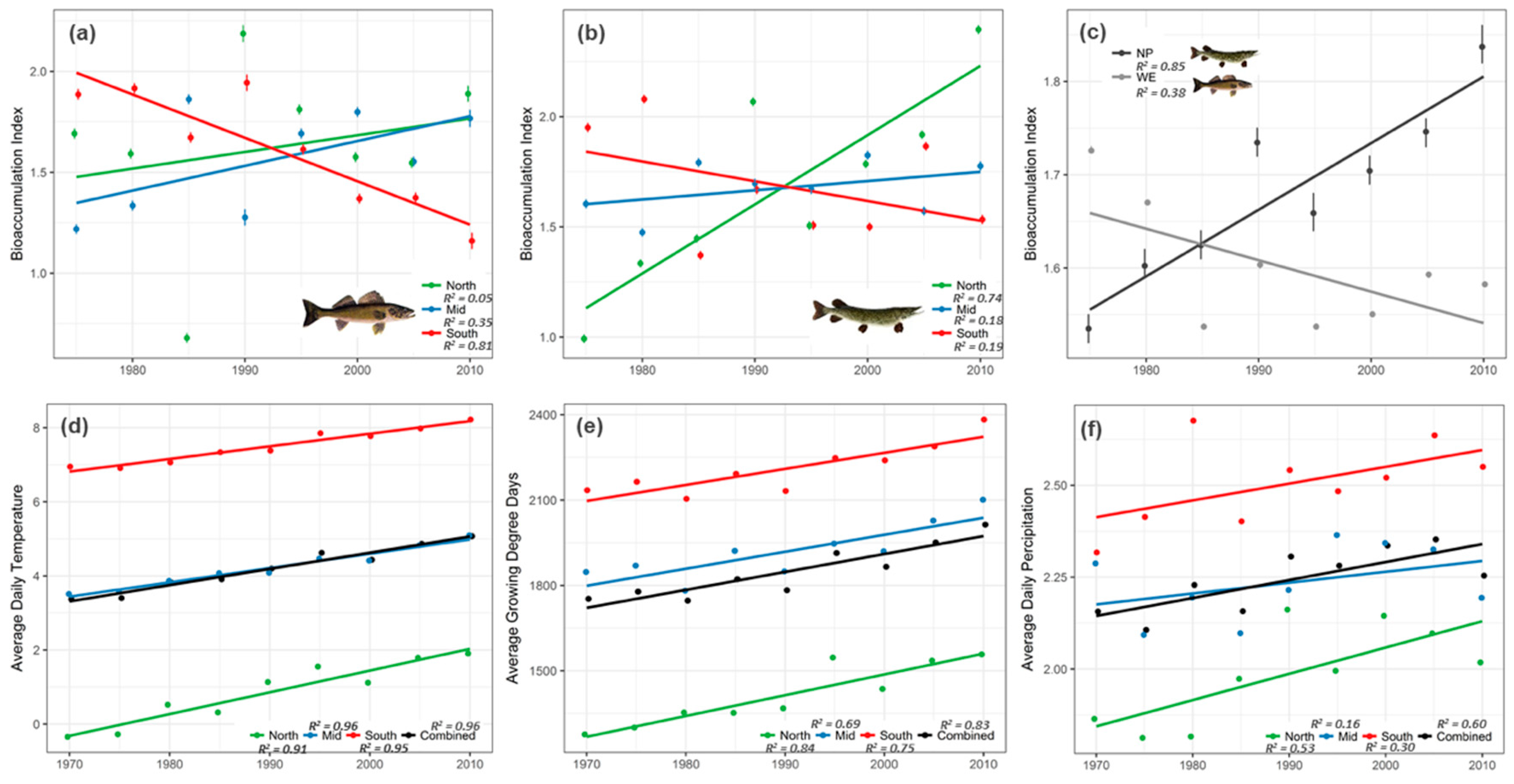
Random slopes of space-time interaction effect (τ_{11, SPATIAL:TEMPORAL}) from the best-fitting full model at broad-scale, signifying magnitude of bioaccumulation (i.e., bioaccumulation index in Figure 3a–c) across 5° latitudinal zones and 5-year time periods, showed spatiotemporal patterns that were overall consistent for both Walleye and Northern Pike (Figure 3a,b). In Walleye, the south latitudinal zone showed strong decline in bioaccumulation with time (β = −0.026; R² = 0.81), whereas the mid zone showed a relatively weak positive trend (β = 0.0083; R² = 0.35) and the north latitude showed a very weak positive trend (β = 0.0045; R² = 0.05). For Northern Pike, bioaccumulation increased strongly with time in north latitudes (β = 0.033; R² = 0.74), while mid latitudes showed a subtle increase (β = 0.0056; R² = 0.18) and south latitudes showed a general decline with time (β = −0.008; R² = 0.19). Overall, both species seem to be bioaccumulating mercury at an increasing rate in the relatively colder latitudinal zones of mid and north, while in the warmer southern latitudes, the rate of bioaccumulation seems to be decreasing. However, it is worth noting that the magnitude of change (slope) was different for these two species, particularly at the extreme latitudes (north and south). Walleye bioaccumulate less mercury much more quickly through time in the southern parts of Ontario, whereas Northern Pike bioaccumulate much more quickly through time in the northern parts of Ontario. We believe these differences have to do with varying species responses to climate change as a result of difference in species biology, which we discuss in more detail below. Unlike spatiotemporal trends that appear similar overall for both Walleye and Northern Pike, a purely temporal perspective (i.e., time as the only random factor; τ_11,TEMPORAL) highlights an interesting dissimilarity with contrasting trends in bioaccumulation: rate of bioaccumulation declined in Walleye over time, whereas Northern Pike showed a strong increase (Figure 3c).

Climate variables showed an overall increasing trend (Figure 3d–f) and this was particularly consistent in the case of average daily temperature (R² = 0.96) and growing degree-days (R² = 0.83). As expected, the overall average (i.e., the intercept) of annual mean temperatures and growing degree-days decreased with increase in latitude. However, it is worth noting that the rate of increase (i.e., the slope) was greatest in northern latitudes (β_temp = 0.06; β_gdd = 7.3) followed by mid (β_temp = 0.04; β_gdd = 5.9) and southern latitudes (β_temp = 0.034; β_gdd = 5.6), suggesting that northern latitudes are warming at a faster rate than southern latitudes, as numerous authors have found [37,38]. Average daily precipitation, like temperature and growing degree-days, showed a generally increasing trend with time, with northern latitudes recording highest rates of increase. However, there was substantial variation during the 45-year time period as evident from the generally lower R² values of precipitation compared to those of temperature and growing degree-days. Also, average daily precipitation was generally greater in southern Ontario relative to mid and northern regions.

3.3. Fine-Scale Variation and Broad-Scale Latitudinal Trends in Fish Growth Rate

The BSM data with age information overall comprised 3159 individual Walleye from 291 waterbodies and 1699 Northern Pike samples from 240 waterbodies across Ontario with latitudes ranging from 44.5° N to 55° N. LMEMs testing for fine-scale differences in Walleye growth rates showed substantial variation associated with waterbody as the random effect (τ_11,WB = 0.196;

Table 5. Summary statistics of LMEMs describing fine-scale (waterbody-level) variation in body mass as a function of age with each unique waterbody sampled treated as a random effect for Walleye and Northern Pike. (Note: numbers in parenthesis show 95% confidence interval).

	log[weight] Walleye	log[weight] Northern Pike
Fixed Parts
${\beta }_0$	4.05 (3.92–4.18)	5.44 (5.36–5.53)
${\beta }_1$ log(age)	1.34 (1.27–1.40)	1.05 (1.00–1.09)
Random Parts
σ2	0.092	0.087
τ00	0.882	0.215
τ11	0.196	0.053
ρ01	−0.896	−0.771
N	291	240
Observations	3159	1699
R2	0.874	0.847

Abbreviations and Symbols: ${\beta }_0$ = overall intercept; ${\beta }_1$ = overall slope of the fixed-effect, log(age); σ² = residual (within-group) variance; τ₀₀ = variance of intercepts for waterbody as random effect; τ₁₁ = variance of slopes (growth rates) for waterbody as random effect; ρ₀₁ = correlation between random slopes and random intercepts; N = number of unique groups (waterbodies) as the random effect; Observations = total number of samples; R² = model r-square.

). In the case of Northern Pike, variation associated with waterbody as random effect were relatively lesser (τ_11,WB = 0.053; Table 5). Put together, fine scale waterbody-specific conditions affect both Walleye and Northern Pike growth rates and it is particularly evident in Walleye.

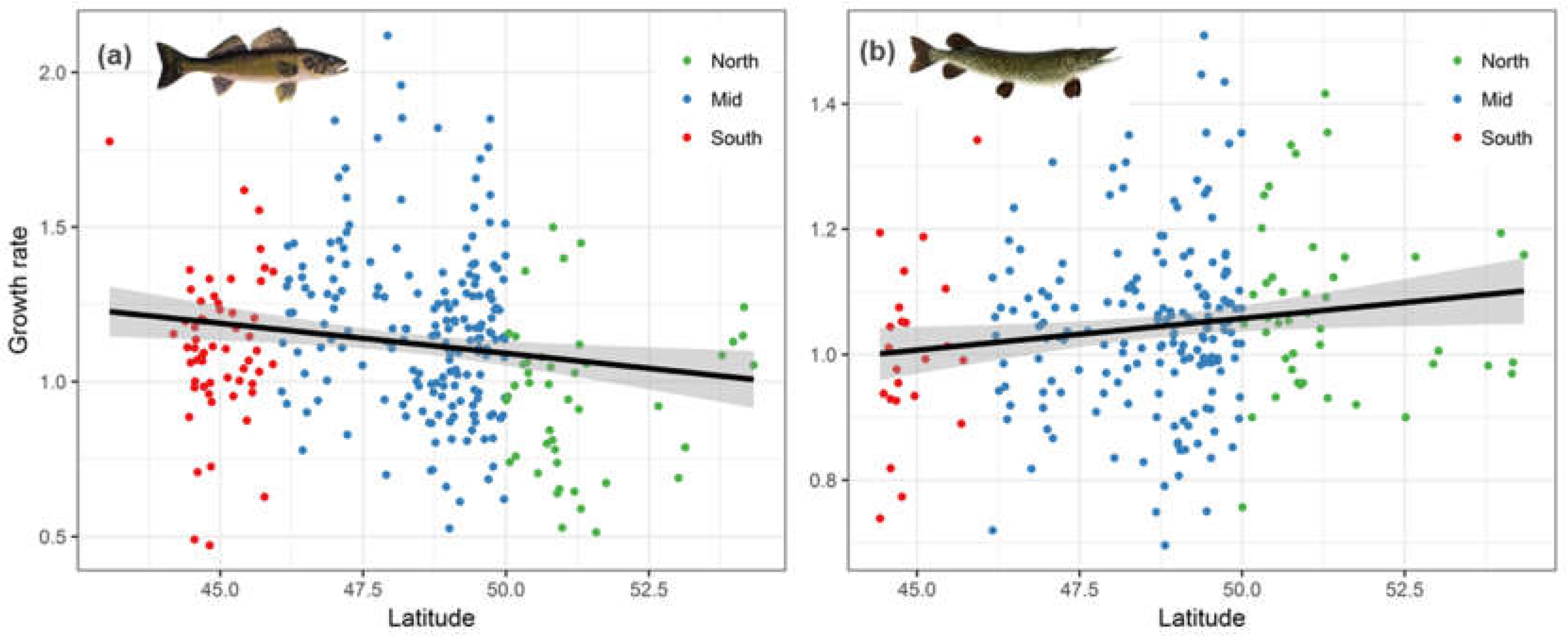
Regressing waterbody-specific growth rate estimates (i.e., τ_11, random slope coefficients) against waterbody latitude revealed weak broad-scale trends (Walleye: p-value = 0.0012 and R² = 0.065; Northern Pike: p-value = 0.051 and R² = 0.015). However, a comparison of these regression results indicates interesting species-specific differences. Stated specifically, the broad-scale trend between growth rate and latitude showed a significant negative relationship in Walleye, suggesting growth rate decreased with latitude overall (Figure 4a), though this relationship may be better captured by a curvilinear fit for Walleye where mid latitudes may be more ‘optimal.’ Even so, the bulk of data for Walleye come from mid and north latitude waterbodies that show decreasing growth rates with increasing latitude, which is consistent with findings in the literature that suggest there is a negative relationship between Walleye growth rates and latitude [39,40]. Northern Pike, on the other hand, showed a barely significant positive relationship between latitude and growth rate (Figure 4b). Also worth noting is the difference in the range of growth rate estimates between the two species; Walleye growth rates ranged from 0.5 to 2.1, while Northern Pike growth rates had relatively narrow range between 0.69 and 1.5. Overall, Walleye growth rates not only showed strong variation across waterbodies but also a discernible latitudinal trend, while Northern Pike growth rates varied relatively less and showed no clear broad-scale latitudinal trend.

Finally, it needs to be stressed that our assessment of magnitude of mercury bioaccumulation (at both fine and broad scales) and fish growth rate (at fine scale only) is based on random-slope estimates of the respective mixed-models. One of the drawbacks of using such estimates is that extreme imbalance in sample sizes across the random-effect groups can potentially lead to an unstable model and biased random-effect estimates [31]. However, large sample size at the individual (fish)-level of the hierarchy can effectively minimize this problem, especially in mixed-models that consider both random intercepts and slopes [32,41]. Hence, we are confident that given the overall large sample size at the fish-level for both mercury bioaccumulation models (49,690 Walleye samples and 32,636 Northern Pike samples) and growth rate models (3159 Walleye samples and 1699 Northern Pike samples), our random group-level estimates are fairly robust.

4. Discussion

In our analyses of fish mercury levels using LMEMs at fine and broad scales, fine-scale models consistently explained more variation than their broad-scale counterparts in both Walleye and Northern Pike, suggesting that environmental factors operating at the individual waterbody level and annual climatic conditions matter more. The best fitting model at both fine- and broad-scales was comprised of spatial, temporal and spatiotemporal interactions as random effects; and among these factors, spatiotemporal interactions captured maximum variation. It is thus evident that mercury bioaccumulation in both Walleye and Northern Pike not only varies spatially across Ontario’s freshwater lakes but this spatial variation interacts with yearly variability and related climatic conditions, such that some lakes or latitudinal zones had much greater fish mercury bioaccumulation rates depending on the year or time period.

In the best-fitting fine-scale model, the spatial component captured variation among waterbodies and had a strong influence on mercury bioaccumulation in addition to space-time interaction effects. The results suggests that mercury bioaccumulation is largely driven by differences in waterbody-specific environmental conditions as they influence both methylmercury generation and fish growth [14]. In this context, it is worth noting that estimated fish growth rates showed similar variations for both Walleye and Northern Pike in models with waterbody as the only random factor (τ₁₁ in Table 5). Previous studies on Walleye and Northern Pike have reported on growth rate variation across lakes due to differences in water chemistry, prey mercury contamination and land use/ disturbances in surrounding catchment areas and these lake-specific growth rate variations modulate fish mercury levels at the population level [42,43]. Thus, it is possible that observed fine-scale variation in mercury bioaccumulation is partly due to variation in fish growth rates at the waterbody-level. From the perspective of managing fish mercury levels, our findings reveal that focusing on waterbody-level conditions that affect fish growth and methyl-mercury generation is critical. Finally and most importantly, the results highlight the overwhelming influence of space-time interactions at fine-scale, which implies annual climate conditions can interact with lake-specific drivers such as water chemistry variables to further modulate methylmercury generation and its uptake by fish. Climate change studies on aquatic ecosystems have reported such potentially complex interactions between climate and hydroecological properties including water chemistry [17,44,45]. The complex nature of these space-time interactions renders long-term projections of fish mercury levels challenging as the effect of both waterbody-specific factors and annual climatic variations needs to be considered simultaneously.

The broad-scale analyses revealed a fairly complex yet tractable spatiotemporal patterns across the 41-year time period and three latitudinal zones for both Walleye and Northern Pike. There were some interesting similarities between species wherein both species showed an overall increasing bioaccumulation trend for north and mid latitudes; whereas south latitudes revealed a decreasing trend (Figure 3a,b). Unlike previous studies, which generally show a declining (or unchanging) trend in both north and south latitudes [8,9,10], our findings showed increasing trends in north latitudes, as was the case for Northern Pike and in mid latitudes, as was the case with Walleye. The reason for this difference in fish mercury trends is perhaps because our definition of bioaccumulation index differs from previous studies that typically measure the rate of change in mercury levels over time. Our measure provides an estimate of the magnitude of bioaccumulation given both latitudinal zone of lake location and temporal period. Moreover, in our analyses bioaccumulation index was based on the full range of fish size to mercury concentration covariation. Like several other long-term studies [8,10,46,47], our results also showed an increase in mercury bioaccumulation for the most recent time periods, particularly in north and mid latitudinal zones (Figure 3a,b). This increase in fish mercury levels in recent periods is speculated to be climate change induced [10,48,49,50]. However, as we shall soon discuss, bioaccumulation trends in the context of climate change suggests complex dynamics that are not easy to generalize. Interestingly, the temporal trends estimated using time period as the only random effect showed contrasting species-specific patterns (Figure 3c), highlighting the importance of considering species-specific responses. Studies on biological indicator species point to the limitations in capturing the complexity of ecosystem responses to various anthropogenic stressors using a single indicator species [51,52].

From a climate change perspective, temperature and growing degree-days showed consistently increasing trends across all latitudinal zones over the 45-year period; while in comparison, mercury bioaccumulation trends varied among latitudinal zones for both Walleye and Northern Pike, with south zones decreasing and north and mid- latitudinal zones increasing to different degrees (Figure 3a,b). It may also be noted that estimated rates of warming did not vary significantly among the three latitudinal zones—though this is perhaps a result of the limited availability of long-term weather data in mid and north latitudinal zones. In the face of nearly similar rates of warming temperature conditions, it is surprising that the latitudinal zone trends in mercury bioaccumulation do not show the same general pattern. This lack of a general pattern suggests that multiple, potentially conflicting, climate-driven factors are involved. More specifically stated, methylation rates may have increased lately, especially in northern latitudes, since methylation in cold northern latitudes is known to occur during the ice-free season when the soil and ground are not frozen [17] and northern latitudes are experiencing a more prolonged ice-free season compared to southern latitudes as a consequence of warming climate [53,54]. Thus the observed increasing trends in fish mercury levels in the relatively colder north and mid latitudes is possibly due to an increase in the rate of methylation in higher latitudes. On the other hand, the generally declining bioaccumulation trend observed for southern latitudes suggests that growth dilution may have an influence in the warm southern temperature conditions, if one assumes that warmer temperatures boost fish growth rates disproportionately relative to metabolism. A similar negative relationship was found in largemouth bass between mercury contamination and temperature in a recent long-term analysis of fish mercury data [13]. The declining bioaccumulation trend in southern latitude may also be attributed to the recent overall reductions in anthropogenic mercury pollution in Canada as a result of stricter environmental regulations [55].

Besides temperature, precipitation is known to affect amount of methylmercury in lakes and waterbodies via surface run-off from surrounding catchment areas [20]. Precipitation in Ontario showed a clear increasing trend in time for all three latitudinal zones with northern latitudes showing the greatest rate of increase in time (Figure 3f). Such increased precipitation, especially brief intense periods of rainfall can result in enhanced methylmercury levels in lakes [56,57]. Thus, the combined effects of longer ice-free season and increased precipitation suggests that lakes and waterbodies in northern latitudes are likely to end up with greater amounts of methylmercury, and consequently higher fish mercury levels over time. Most importantly, when these climate change effects are juxtaposed with recent findings that suggest permafrost in northern latitudes potentially hold some of the largest known reservoirs of mercury [58], it is indeed possible that the impact of mercury on ecosystems and human well-being could be far more severe in the future.

The contrasting temporal trends in bioaccumulation within Ontario’s warming climate setting is indicative of species-specific ecological differences (Figure 3c). In Walleye, the declining bioaccumulation temporal trend suggests growth dilution is a potential mechanism provided warming temperature enhances growth rate more than metabolism. While we have no evidence regarding the effect of warming temperature on Walleye’s metabolism, it is indeed possible that Walleye growth rate increases with temperature. This is supported by the weak but discernible negative latitudinal growth rate (i.e., higher growth rate in waterbodies at warmer latitudes) found in Walleye (Figure 4a); and also by previous studies that similarly demonstrated a negative relationship between latitude and growth rates in Walleye [39,40]. The negative relationship between latitude and fish growth rate is largely the consequence of several temperature-dependent physiological processes operating at the molecular-level such as enzymatic reaction rates, which eventually affect fish metabolism and growth [59]. The temperature-driven increase in Walleye metabolism can also increase consumption rate, which may further interact with waterbody specific factors such as contaminated prey availability, thus potentially decreasing the net possibility of temperature-driven growth dilution in Walleye [60]. In Northern Pike, the temporal trend in bioaccumulation showed a strong and consistent increase with time, whereas growth rate showed no clear correlation with latitude, which suggests temperature-driven growth dilution is highly unlikely. In a previous broad-scale analysis of Northern Pike data, growth rate was found to be negatively correlated with latitude [61]. However, Rypel’s meta-analysis considered nearly 30 degrees of latitudinal variation while our study ranges between 45 and 55 latitudinal degrees, thus potentially capturing much lesser variation in growth. Rypel also points to the importance of scale when considering the effect of climate change on growth rate for cool-water species such as Walleye and Northern Pike. In short, the effects of climate warming on growth rates of cool-water fishes is likely to be highly variable and scale-dependent. Along these lines, it is worth noting that our results on the correlation between growth rate and latitude have very low R-square values for both Walleye and Northern Pike, which again suggests that growth rate is more locally modulated at the waterbody-level. Thus, the low R-square values imply temperature-driven variation in growth rate does not fully explain the observed temporal bioaccumulation trends. To that effect, there are other factors besides latitudinal (temperature driven) variation in growth rate, such as species-specific differences in feeding habits, prey choice and predatory behavior that might better explain the observed contrasting mercury bioaccumulation trends in time between Walleye and Northern Pike. Prior research have reported disparities between Walleye and Northern Pike in mercury loads as a result of differences in the feeding habits of these two co-occurring fishes [62,63].

5. Conclusions

Our study provides a detailed scale-specific assessment of mercury bioaccumulation in space and time for two common freshwater sport fishes. While much of the variation in mercury bioaccumulation was captured at fine-scale of waterbody- and year-level, the broad-scale analysis summarizes the fine-scale variations within a climate change context. The study also demonstrates how a simple bioaccumulation index derived from mixed-effects models can capture broad-scale spatiotemporal patterns of fish mercury bioaccumulation. A key finding was the significance of spatiotemporal interactions in determining mercury bioaccumulation at both fine and broad scales of analysis, which suggests that future studies should consider characterizing and quantifying the many latent interactions among the various spatial and temporal drivers that affect mercury bioaccumulation in fishes; such as the effect of annual temperature conditions on lake water chemistry and fish growth/metabolism and at broad-scales, the generally warming conditions.

References

- Kudo, A.; Fujikawa, Y.; Miyahara, S.; Zheng, J.; Takigami, H.; Sugahara, M.; Muramatsu, T. Lessons from Minamata mercury pollution, Japan—After a continuous 22 years of observation. Water Sci. Technol. 1998, 38, 187–193. [Google Scholar] [CrossRef]
- Novick, S. A new pollution problem. Environ. Sci. Policy Sustain. Dev. 1969, 11, 2–9. [Google Scholar] [CrossRef]
- Vecsey, C. Grassy narrows reserve: Mercury pollution, social disruption, and natural resources: A question of autonomy. Am. Indian Q. 1987, 11, 287–314. [Google Scholar] [CrossRef]
- Driscoll, C.T.; Mason, R.P.; Chan, H.M.; Jacob, D.J.; Pirrone, N. Mercury as a global pollutant: Sources, pathways, and effects. Environ. Sci. Technol. 2013, 47, 4967–4983. [Google Scholar] [CrossRef] [PubMed]
- Selin, N.E. Global biogeochemical cycling of mercury: A review. Annu. Rev. Environ. Resour. 2009, 34, 43–63. [Google Scholar] [CrossRef]
- Sundseth, K.; Pacyna, J.M.; Pacyna, E.G.; Pirrone, N.; Thorne, R.J. Global sources and pathways of mercury in the context of human health. Int. J. Environ. Res. Public Health 2017, 14, 105. [Google Scholar] [CrossRef] [PubMed]
- Boening, D.W. Ecological effects, transport, and fate of mercury: A general review. Chemosphere 2000, 40, 1335–1351. [Google Scholar] [CrossRef]
- Chalmers, A.T.; Argue, D.M.; Gay, D.A.; Brigham, M.E.; Schmitt, C.J.; Lorenz, D.L. Mercury trends in fish from rivers and lakes in the United States, 1969–2005. Environ. Monit. Assess. 2011, 175, 175–191. [Google Scholar] [CrossRef] [PubMed]
- Monson, B.A.; Staples, D.F.; Bhavsar, S.P.; Holsen, T.M.; Schrank, C.S.; Moses, S.K.; McGoldrick, D.J.; Backus, S.M.; Williams, K.A. Spatiotemporal trends of mercury in walleye and largemouth bass from the Laurentian Great Lakes region. Ecotoxicology 2011, 20, 1555–1567. [Google Scholar] [CrossRef] [PubMed]
- Gandhi, N.; Tang, R.W.; Bhavsar, S.P.; Arhonditsis, G.B. Fish mercury levels appear to be increasing lately: A report from 40 years of monitoring in the province of Ontario, Canada. Environ. Sci. Technol. 2014, 48, 5404–5414. [Google Scholar] [CrossRef] [PubMed]
- Kamman, N.C.; Burgess, N.M.; Driscoll, C.T.; Simonin, H.A.; Goodale, W.; Linehan, J.; Estabrook, R.; Hutcheson, M.; Major, A.; Scheuhammer, A.M.; et al. Mercury in freshwater fish of northeast North America–a geographic perspective based on fish tissue monitoring databases. Ecotoxicology 2005, 14, 163–180. [Google Scholar] [CrossRef] [PubMed]
- Gandhi, N.; Bhavsar, S.P.; Tang, R.W.; Arhonditsis, G.B. Projecting fish mercury levels in the province of Ontario, Canada and the implications for fish and human health. Environ. Sci. Technol. 2015, 49, 14494–14502. [Google Scholar] [CrossRef] [PubMed]
- Chen, M.M.; Lopez, L.; Bhavsar, S.P.; Sharma, S. What’s hot about mercury? Examining the influence of climate on mercury levels in Ontario top predator fishes. Environ. Res. 2018, 162, 63–73. [Google Scholar] [CrossRef] [PubMed]
- Ward, D.M.; Nislow, K.H.; Folt, C.L. Bioaccumulation syndrome: Identifying factors that make some stream food webs prone to elevated mercury bioaccumulation. Ann. N. Y. Acad. Sci. 2010, 1195, 62–83. [Google Scholar] [CrossRef] [PubMed]
- Scheuhammer, A.M.; Meyer, M.W.; Sandheinrich, M.B.; Murray, M.W. Effects of environmental methylmercury on the health of wild birds, mammals, and fish. AMBIO A J. Hum. Environ. 2007, 36, 12–19. [Google Scholar] [CrossRef]
- Canário, J.; Branco, V.; Vale, C. Seasonal variation of monomethylmercury concentrations in surface sediments of the Tagus Estuary (Portugal). Environ. Pollut. 2007, 148, 380–383. [Google Scholar] [CrossRef] [PubMed]
- Stern, G.A.; Macdonald, R.W.; Outridge, P.M.; Wilson, S.; Chetelat, J.; Cole, A.; Hintelmann, H.; Loseto, L.L.; Steffen, A.; Wang, F.; et al. How does climate change influence arctic mercury? Sci. Total Environ. 2012, 414, 22–42. [Google Scholar] [CrossRef] [PubMed]
- Kidd, K.A.; Muir, D.C.; Evans, M.S.; Wang, X.; Whittle, M.; Swanson, H.K.; Johnston, T.; Guildford, S. Biomagnification of mercury through lake trout (Salvelinus namaycush) food webs of lakes with different physical, chemical and biological characteristics. Sci. Total Environ. 2012, 438, 135–143. [Google Scholar] [CrossRef] [PubMed]
- Lavoie, R.A.; Jardine, T.D.; Chumchal, M.M.; Kidd, K.A.; Campbell, L.M. Biomagnification of mercury in aquatic food webs: A worldwide meta-analysis. Environ. Sci. Technol. 2013, 47, 13385–13394. [Google Scholar] [CrossRef] [PubMed]
- Rudd, J.W. Sources of methyl mercury to freshwater ecosystems: A review. Water Air Soil Pollut. 1995, 80, 697–713. [Google Scholar] [CrossRef]
- Dijkstra, J.A.; Buckman, K.L.; Ward, D.; Evans, D.W.; Dionne, M.; Chen, C.Y. Experimental and natural warming elevates mercury concentrations in estuarine fish. PLoS ONE 2013, 8, e58401. [Google Scholar] [CrossRef] [PubMed]
- Karimi, R.; Chen, C.Y.; Pickhardt, P.C.; Fisher, N.S.; Folt, C.L. Stoichiometric controls of mercury dilution by growth. Proc. Natl. Acad. Sci. USA 2007, 104, 7477–7482. [Google Scholar] [CrossRef] [PubMed] [Green Version]
- Greenfield, B.K.; Hrabik, T.R.; Harvey, C.J.; Carpenter, S.R. Predicting mercury levels in yellow perch: Use of water chemistry, trophic ecology, and spatial traits. Can. J. Fish. Aquat. Sci. 2001, 58, 1419–1429. [Google Scholar] [CrossRef]
- Gorski, P.R.; Cleckner, L.B.; Hurley, J.P.; Sierszen, M.E.; Armstrong, D.E. Factors affecting enhanced mercury bioaccumulation in inland lakes of Isle Royale National Park, USA. Sci. Total Environ. 2003, 304, 327–348. [Google Scholar] [CrossRef]
- Swenson, W.A. Food consumption of walleye (Stizostedion vitreum vitreum) and sauger (S. canadense) in relation to food availability and physical conditions in Lake of the Woods, Minnesota, Shagawa Lake, and western Lake Superior. J. Fish. Board Can. 1977, 34, 1643–1654. [Google Scholar] [CrossRef]
- Casselman, J.M.; Lewis, C.A. Habitat requirements of northern pike (Essox lucius). Can. J. Fish. Aquat. Sci. 1996, 53, 161–174. [Google Scholar] [CrossRef]
- Nasr, M.; Arp, P.A. Mercury and organic matter concentrations in lake and stream sediments in relation to one another and to atmospheric mercury deposition and climate variations across Canada. J. Chem. 2017, 2017, 8949502. [Google Scholar] [CrossRef]
- Hallett, T.B.; Coulson, T.; Pilkington, J.G.; Clutton-Brock, T.H.; Pemberton, J.M.; Grenfell, B.T. Why large-scale climate indices seem to predict ecological processes better than local weather. Nature 2004, 430, 71. [Google Scholar] [CrossRef] [PubMed]
- Gewurtz, S.B.; Bhavsar, S.P.; Fletcher, R. Influence of fish size and sex on mercury/PCB concentration: Importance for fish consumption advisories. Environ. Int. 2011, 37, 425–434. [Google Scholar] [CrossRef] [PubMed]
- Bolker, B.M.; Brooks, M.E.; Clark, C.J.; Geange, S.W.; Poulsen, J.R.; Stevens, M.H.H.; White, J.S.S. Generalized linear mixed models: A practical guide for ecology and evolution. Trends Ecol. Evol. 2009, 24, 127–135. [Google Scholar] [CrossRef] [PubMed]
- Harrison, X.A.; Donaldson, L.; Correa-Cano, M.E.; Evans, J.; Fisher, D.N.; Goodwin, C.E.; Robinson, B.S.; Hodgson, D.J.; Inger, R. A brief introduction to mixed effects modelling and multi-model inference in ecology. PeerJ 2018, 6, e4794. [Google Scholar] [CrossRef] [PubMed]
- Wagner, T.; Fergus, C.E.; Stow, C.A.; Cheruvelil, K.S.; Soranno, P.A. The statistical power to detect cross-scale interactions at macroscales. Ecosphere 2016, 7, e01417. [Google Scholar] [CrossRef]
- Bates, D.; Maechler, M.; Bolker, B.; Walker, S. lme4: Linear Mixed-Effects Models Using Eigen and S4; R Package Version. J. Stat. Softw. 2015, 67, 1–48. [Google Scholar] [CrossRef]
- Knowles, J.; Frederick, C. merTools: Tools for Analyzing Mixed Effect Regression Models, R Package Version 0.1.0; 2016. Available online: https://cran.r-project.org/web/packages/merTools/index.html (accessed on 5 April 2018).
- R Core Team. R: A Language and Environment for Statistical Computing; R Foundation for Statistical Computing: Vienna, Austria, 2018; Available online: https://www.R-project.org/ (accessed on 1 March 2018).
- Lester, N.P.; Marshall, T.R.; Armstrong, K.; Dunlop, W.I.; Ritchie, B. A broad-scale approach to management of Ontario’s recreational fisheries. North Am. J. Fish. Manag. 2003, 23, 1312–1328. [Google Scholar] [CrossRef]
- Schwartz, M.D.; Ahas, R.; Aasa, A. Onset of spring starting earlier across the Northern Hemisphere. Glob. Chang. Biol. 2006, 12, 343–351. [Google Scholar] [CrossRef]
- Freidman, A.R.; Hwang, Y.T.; Chiang, J.C.; Frierson, D.M. Interhemispheric temperature asymmetry over the twentieth century and in future projections. J. Clim. 2013, 26, 5419–5433. [Google Scholar] [CrossRef]
- Quist, M.C.; Guy, C.S.; Schultz, R.D.; Stephen, J.L. Latitudinal comparisons of walleye growth in North America and factors influencing growth of walleyes in Kansas reservoirs. N. Am. J. Fish. Manag. 2003, 23, 677–692. [Google Scholar] [CrossRef]
- Lavigne, M.; Lucotte, M.; Paquet, S. Relationship between mercury concentration and growth rates for walleyes, northern pike, and lake trout from Quebec lakes. N. Am. J. Fish. Manag. 2010, 30, 1221–1237. [Google Scholar] [CrossRef]
- Grueber, C.E.; Nakagawa, S.; Laws, R.J.; Jamieson, I.G. Multimodel inference in ecology and evolution: Challenges and solutions. J. Evol. Boil. 2011, 24, 699–711. [Google Scholar] [CrossRef] [PubMed]
- Garcia, E.; Carignan, R. Mercury concentrations in northern pike (Esox lucius) from boreal lakes with logged, burned, or undisturbed catchments. Can. J. Fish. Aquat. Sci. 2000, 57, 129–135. [Google Scholar] [CrossRef]
- Simoneau, M.; Lucotte, M.; Garceau, S.; Laliberté, D. Fish growth rates modulate mercury concentrations in walleye (Sander vitreus) from eastern Canadian lakes. Environ. Res. 2005, 98, 73–82. [Google Scholar] [CrossRef] [PubMed]
- Prowse, T.D.; Wrona, F.J.; Reist, J.D.; Gibson, J.J.; Hobbie, J.E.; Lévesque, L.M.; Vincent, W.F. Climate change effects on hydroecology of Arctic freshwater ecosystems. AMBIO A J. Hum. Environ. 2006, 35, 347–358. [Google Scholar] [CrossRef]
- Frey, K.E.; McClelland, J.W. Impacts of permafrost degradation on arctic river biogeochemistry. Hydrol. Process. Int. J. 2009, 23, 169–182. [Google Scholar] [CrossRef]
- Sadraddini, S.; Azim, M.E.; Shimoda, Y.; Mahmood, M.; Bhavsar, S.P.; Backus, S.M.; Arhonditsis, G.B. Temporal PCB and mercury trends in Lake Erie fish communities: A dynamic linear modeling analysis. Ecotoxicol. Environ. Saf. 2011, 74, 2203–2214. [Google Scholar] [CrossRef] [PubMed]
- Blukacz-Richards, E.A.; Visha, A.; Graham, M.L.; McGoldrick, D.L.; de Solla, S.R.; Moore, D.J.; Arhonditsis, G.B. Mercury levels in herring gulls and fish: 42 years of spatio-temporal trends in the Great Lakes. Chemosphere 2017, 172, 476–487. [Google Scholar] [CrossRef] [PubMed]
- Monson, B.A. Trend reversal of mercury concentrations in piscivorous fish from Minnesota Lakes: 1982−2006. Environ. Sci. Technol. 2009, 43, 1750–1755. [Google Scholar] [CrossRef] [PubMed]
- Rigét, F.; Vorkamp, K.; Muir, D. Temporal trends of contaminants in Arctic char (Salvelinus alpinus) from a small lake, southwest Greenland during a warming climate. J. Environ. Monit. 2010, 12, 2252–2258. [Google Scholar] [CrossRef] [PubMed]
- Carrie, J.; Wang, F.; Sanei, H.; Macdonald, R.W.; Outridge, P.M.; Stern, G.A. Increasing contaminant burdens in an Arctic fish, burbot (Lota lota), in a warming climate. Environ. Sci. Technol. 2009, 44, 316–322. [Google Scholar] [CrossRef] [PubMed]
- Carignan, V.; Villard, M.A. Selecting indicator species to monitor ecological integrity: A review. Environ. Monit. Assess. 2002, 78, 45–61. [Google Scholar] [CrossRef] [PubMed]
- Siddig, A.A.; Ellison, A.M.; Ochs, A.; Villar-Leeman, C.; Lau, M.K. How do ecologists select and use indicator species to monitor ecological change? Insights from 14 years of publication in Ecological Indicators. Ecol. Indic. 2016, 60, 223–230. [Google Scholar] [CrossRef] [Green Version]
- Schindler, D.W.; Beaty, K.G.; Fee, E.J.; Cruikshank, D.R.; DeBruyn, E.R.; Findlay, D.L.; Linsey, G.A.; Shearer, J.A.; Stainton, M.P.; Turner, M.A. Effects of climatic warming on lakes of the central boreal forest. Science 1990, 250, 967–970. [Google Scholar] [CrossRef] [PubMed]
- Duguay, C.R.; Prowse, T.D.; Bonsal, B.R.; Brown, R.D.; Lacroix, M.P.; Ménard, P. 7 Recent trends in Canadian lake ice cover. Hydrol. Process. 2006, 20, 781–801. [Google Scholar] [CrossRef]
- Muir, D.C.G.; Wang, X.; Yang, F.; Nguyen, N.; Jackson, T.A.; Evans, M.S.; Douglas, M.; Kock, G.; Lamoureux, S.; Pienitz, R.; et al. Spatial trends and historical deposition of mercury in eastern and northern Canada inferred from lake sediment cores. Environ. Sci. Technol. 2009, 43, 4802–4809. [Google Scholar] [CrossRef] [PubMed]
- Matilainen, T.; Verta, M.; Korhonen, H.; Uusi-Rauva, A.; Niemi, M. Behavior of mercury in soil profiles: Impact of increased precipitation, acidity, and fertilization on mercury methylation. Water Air Soil Pollut. 2001, 125, 105–120. [Google Scholar] [CrossRef]
- Balogh, S.J.; Swain, E.B.; Nollet, Y.H. Elevated methylmercury concentrations and loadings during flooding in Minnesota rivers. Sci. Total Environ. 2006, 368, 138–148. [Google Scholar] [CrossRef] [PubMed]
- Schuster, P.F.; Schaefer, K.M.; Aiken, G.R.; Antweiler, R.C.; Dewild, J.F.; Gryziec, J.D.; Gusmeroli, A.; Hugelius, G.; Jafarov, E.; Krabbenhoft, D.P.; et al. Permafrost stores a globally significant amount of mercury. Geophys. Res. Lett. 2018, 45, 1463–1471. [Google Scholar] [CrossRef]
- Uphoff, C.S.; Schoenebeck, C.W.; Hoback, W.W.; Koupal, K.D.; Pope, K.L. Degree-day accumulation influences annual variability in growth of age-0 walleye. Fish. Res. 2013, 147, 394–398. [Google Scholar] [CrossRef] [Green Version]
- Galarowicz, T.L.; Wahl, D.H. Differences in growth, consumption, and metabolism among walleyes from different latitudes. Trans. Am. Fish. Soc. 2003, 132, 425–437. [Google Scholar] [CrossRef]
- Rypel, A.L. Meta-analysis of growth rates for a circumpolar fish, the Northern Pike (Esox lucius), with emphasis on effects of continent, climate and latitude. Ecol. Freshw. Fish 2012, 21, 521–532. [Google Scholar] [CrossRef]
- Mathers, R.A.; Johansen, P.H. The effects of feeding ecology on mercury accumulation in walleye (Stizostedion vitreum) and pike (Esox lucius) in Lake Simcoe. Can. J. Zoöl. 1985, 63, 2006–2012. [Google Scholar] [CrossRef]
- Wren, C.D.; Scheider, W.A.; Wales, D.L.; Muncaster, B.W.; Gray, I.M. Relation between mercury concentrations in walleye (Stizostedion vitreum vitreum) and northern pike (Esox lucius) in Ontario lakes and influence of environmental factors. Can. J. Fish. Aquat. Sci. 1991, 48, 132–139. [Google Scholar] [CrossRef]
Figure 1.
Long-term distribution of fish mercury samples for (a) Walleye and (b) Northern Pike ranging from 1975–2015 gathered by Ontario Ministry of Environment, Conservation and Parks (OMECP).
Figure 2.
Distribution of (a) Walleye and (b) Northern Pike samples across the three defined latitudinal zones in Ontario obtained from the Broad Scale Monitoring program’s first sampling cycle between 2008 and 2012.
Figure 3.
Spatiotemporal trends of mercury bioaccumulation in (a) Walleye and (b) Northern Pike as predicted by the random slopes of the full model with time period and latitudinal zone interactions as random effects. Temporal trends in bioaccumulation for both Walleye and Northern Pike are shown in (c) as the predicted random slopes of the full model with time period alone as the random effect. Error bars indicate ± 1SD. Change in climatic conditions are shown as spatiotemporal trends in (d) temperature, (e) growing degree days and (f) precipitation based on average measures at Environment Canada sampling stations, estimated from aggregated 5-year time periods.
Figure 4.
Latitudinal variation in growth rate of (a) Walleye (R2 = 0.065; p-value = 0.0012) and (b) Northern Pike (R2 = 0.015; p-value = 0.051) expressed as random slopes of LMEMs of fish growth model (Equation (2) in text) with each unique waterbody as the random effect. Shaded area indicates 95% confidence interval. (Note: y-axis scale differs between a and b).