Article

Segmentation of Apples in Aerial Images under Sixteen Different Lighting Conditions Using Color and Texture for Optimal Irrigation

by
Sajad Sabzi
1,
Yousef Abbaspour-Gilandeh
1,*,
Ginés García-Mateos
2,*,
Antonio Ruiz-Canales
3 and
José Miguel Molina-Martínez
4
1
Department of Biosystems Engineering, College of Agriculture, University of Mohaghegh Ardabili, Ardabil 56199-11367, Iran
2
Computer Science and Systems Department, University of Murcia, 30100 Murcia, Spain
3
Engineering Department, Miguel Hernandez University of Elche, 03312 Orihuela, Spain
4
Food Engineering and Agricultural Equipment Department, Technical University of Cartagena, 30203 Cartagena, Spain
*
Authors to whom correspondence should be addressed.
Water 2018, 10(11), 1634; https://doi.org/10.3390/w10111634
Submission received: 25 September 2018 / Revised: 1 November 2018 / Accepted: 7 November 2018 / Published: 12 November 2018
(This article belongs to the Special Issue Water Management Using Drones and Satellites in Agriculture)

Abstract

:
Due to the changes in the lighting intensity and conditions throughout the day, machine vision systems used in precision agriculture for irrigation management should be prepared for all possible conditions. For this purpose, a complete segmentation algorithm has been developed for a case study on apple fruit segmentation in outdoor conditions using aerial images. This algorithm has been trained and tested using videos with 16 different light intensities from apple orchards during the day. The proposed segmentation algorithm consists of five main steps: (1) transforming frames in RGB to CIE L*u*v* color space and applying thresholds on image pixels; (2) computing texture features of local standard deviation; (3) using intensity transformation to remove background pixels; (4) color segmentation applying different thresholds in RGB space; and (5) applying morphological operators to refine the results. During the training process of this algorithm, it was observed that frames in different light conditions had more than 58% color sharing. Results showed that the accuracy of the proposed segmentation algorithm is higher than 99.12%, outperforming other methods in the state of the art that were compared. The processed images are aerial photographs like those obtained from a camera installed in unmanned aerial vehicles (UAVs). This accurate result will enable more efficient support in the decision making for irrigation and harvesting strategies.

1. Introduction

Segmentation is an important step in designing machine vision systems for agricultural and gardening purposes. Moreover, it is one of the most difficult and critical parts of such systems, since background can contain objects with a wide variety of colors and textures similar to those of the plants. Incorrect segmentation involves part of the background being considered as the object of interest, and vice versa [1], thus reducing accuracy of the subsequent machine vision processes.
In general, segmentation has been applied in problems such as identifying plant species [2], determining the growth state of the crop [3], and detecting plant diseases in images [4]. Usually, image-based segmentation techniques consist of two main steps: preprocessing the image, and classifying the pixels [5]. Classification is easier in applications with few background objects and artificial light conditions than in situations with many background objects and large color variations. Dorj et al. [6] stated that estimating the production of citrus before harvesting is an important step in predicting the space required for packaging, storing, and marketing. Due to the lack of tools to estimate citrus trees production, this is currently done manually with low accuracy. Therefore, they believe that using an image processing system would allow automatic estimation. For this reason, they presented a method for recognizing trees and counting the number of fruits on them. The citrus counting algorithm consists of these stages: conversion of RGB images to HSV color space; thresholding these images; identification of orange color; noise removal; application of watershed segmentation; and counting. The experiments indicated that the determination coefficient between the samples identified manually and with the algorithm was 0.93.
In another study, Behroozi-Khazaei and Maleki [7] pointed out that using image processing for garden operations, especially in segmentation, is a very challenging problem. They proposed an algorithm for the segmentation of ripe grape clusters from leaves and background based on color features, using artificial neural networks and genetic algorithms. Their database included 129 images which are publicly available. Their results showed that the overall accuracy of the segmentation algorithm was 99.4%.
Diseases in crops, herbs, and other plants reduce production and, hence, farmers’ income. These diseases usually result in color changes, leaf spots, and veins. Identifying these diseases in initial stages of growth helps combating and destroying them. Hu et al. [8] proposed a segmentation method for diagnosing wheat leaf lesions using optimized multi- channel based on the Chan-Vese model. For training the proposed algorithm, 55 images were taken in a day under natural light conditions at a resolution of 3072 × 2304 pixels. The first step of analysis extracts three color channels with principal component analysis (PCA) from the six channels of RGB and HSV color spaces, in order to use full color information. In the next step, k-means method is used to get the initial lesion curve. Their results showed that accuracy of segmentation for HSV and RGB was 79.02% and 82.57%, respectively, which is 15.5% and 60.1% less than the results of the method extracting three color channels using PCA.
Moreover, these applications include algorithms to segment vegetation from soil and distinguish between healthy and stressed crops, as for example wheat. In many cases, digital images are taken in the field and later processed on a desktop computer. In other cases, the device includes a wireless camera with near real-time computer vision capabilities and desktop computer [9]. On the other hand, Singh and Misra [10] proposed an automatic segmentation algorithm for identification and segmentation of different plant and tree leaf diseases. The proposed method performs segmentation based on genetic algorithms. Different steps of their algorithm include: taking images with a digital camera; preprocessing input images for increasing quality and removing unwanted distortion of the image; masking most of the green pixels; removing masked cells within the borders of contaminated clusters; and getting useful segmentation for classifying various leaf diseases.
One of the most important applications of machine vision systems in agriculture is the estimation of crop evapotranspiration for optimal irrigation purposes and some related parameters. The basis of these systems is also a segmentation algorithm. Varied applications can be found in the current literature. One of the main uses is the measuring of the canopy temperature distribution within trees [11]. Another application is for testing the moisture content in leaves of lettuce samples [12]. In this regard, Hernández-Hernández et al. [13] proposed a method for choosing the optimal color space for plant segmentation in the agricultural domain. To train the proposed algorithm, they took 182 images of two kinds of lettuce (var. Iron and Little Gem) and kohlrabi (var. Gongylodes) using a digital camera in four different conditions of direct sunlight and clouds. They proposed a method for training a color model based on different color spaces including RGB, HSL, YCbCr, YUV, L*a*b*, L*u*v*, TSL, I1I2I3, and XYZ. The best color space is automatically selected depending on the case of study. Finally, the pixels are classified as plant/soil by a probabilistic color model using normalized histograms in the selected space. Classification results indicate that the proposed model has an excellent accuracy, with an error of only 0.5% in the estimation of the percentage of green cover, which is later used for irrigation purposes. In another study, Li et al. [14] used a segmentation algorithm to detect cotton in a field. This algorithm was trained under supervised and unsupervised conditions. The first step employs simple linear iterative clustering (SLIC) and density-based spatial clustering for applications with noise (DBSCAN), to generate superpixel regions which preserve edges. Then, color and texture features are extracted from these regions, and the accuracy of cotton diagnosis is assessed. The obtained results show that the proposed algorithm achieves an error of 0.45% on the 42 test images.
The main objective of the present research is to design a new algorithm to segment apples on trees using images extracted from video under 16 different natural light conditions. The use of this segmentation may be varied—e.g., detection of fruits for harvesting, calculation of the maturity state of the fruit, among others—but in this case it is centered in the estimation of the volume of the canopy that includes fruits, and the volume of the canopy that includes leaves and branches, compared to a manual analysis of the images. This information can be used for detecting the difference of the crop evapotranspiration in fruit trees and obtain a highly precise crop water demand. As described above, the previous studies on segmentation in agriculture have three main deficiencies, which are addressed in the proposed method. The first general problem is the low number of images used for training and testing the proposed algorithms, which has reduced their reliability. Second, most works use high-quality images captured in static mode; however, in many garden operations such as spraying, the process must be applied in motion, resulting in low quality images. The proposed method should be prepared for these conditions. Third, little research has been done on photographs taken throughout day. Since light conditions change continuously during the day, the more the frequency of filming, the more robust and accurate the algorithm training. It is interesting to observe that the improvement in the accuracy of segmentation will be beneficial for the subsequent processes of crop monitoring, yield estimate and irrigation scheduling, among others.

2. Materials and Methods

In general, the development of a new computer vision system involves the analysis and validation of different techniques and features, before defining the steps of the proposed system. Depending on the application, the segmentation algorithm can be the main stage of the process, or just a preliminary step followed by other computations. Figure 1 shows a global outline of the methodology used for creating the new algorithm for apple color segmentation. The steps of this process are described in the following subsections, as indicated in the figure.

2.1. Video Recording Under 16 Different Lighting Conditions

It is well known that light intensity changes continuously throughout the day. This must be added to the weather conditions, which can vary from sunny to very cloudy. Thus, segmentation algorithms should offer high accuracy in all conditions, so they should be trained under all possible light intensities. In the present study, a digital camera (DFK 23GM021, CMOS, 120 f/s, Imaging Source GmbH, Bremen, Germany) has been used to record video sequences. The light intensity of each video was measured before filming using a TES 1339R Light Meter Pro (TES Electrical Electronic Corp., Taipei, Taiwan). The videos were captured on 16 different days, with different times of day and weather conditions, as described in Table 1. These videos are a representative sample of the most common conditions in the area of study. Figure 2 shows a sample frame for each of these cases. It can be observed that capture conditions (height and viewing angle) emulate aerial photographs obtained from cameras installed in unmanned aerial vehicles (UAVs), flying at low altitude in order to have a direct view of the fruits. In a drone flying at a high altitude and with a top view of the camera, the fruits could not be seen as they would be too small and covered by the canopy. Due to the unavailability of the drone, filming in this experiment was done by hand. The distance to the trees was variable from 0.5 m to 2 m, and the viewing angle was 90 degrees, i.e., parallel to the ground. The trees filmed each day are different and 5 distinct orchards were used in total. The videos were always captured in daylight hours and the wind speed was very low or zero. After capture, the sample frames are randomly divided in 70% for training the proposed algorithms, and the remaining 30% for test and validation (15% each of them).

2.2. Analysis of Color Spaces

Some authors have pointed out the importance of selecting the optimal color space for each case of interest in segmentation problems [15]. One color space could be effective depending on the problem domain and the classifier applied. In this study 17 different color spaces have been analyzed: RGB, HSV, YIQ, YCbCr, CMY, HSI, Improved YCbCr, L*a*b*, JPEG-YCbCr, YDbDr, YPbPr, YUV, HSL, XYZ, L*u*v*, LCH and CAT02 LMS. The definition of these color spaces can be found in [15,16]. Since each color space includes three channels, a total of 51 color channels are obtained for each pixel (although some of them can be repeated, such as H in HSV, his, and HSL). The purpose is to find the optimal and minimal selection of channels to be used as a part of the segmentation process.

2.3. Analysis of Texture Features

In addition to color, texture can offer other valuable information to discriminate the objects of interest from the background. Each object can have different kinds of typical textures. Many methods have been proposed to represent texture, using different approaches. One of the most common divisions is between soft and hard textures. In this context, soft textures are those that contain homogeneous object pixels, and hard textures are those with heterogeneous object pixels. Since the background of extracted video frames contains different objects, such as leaves and small branches, and each object has a unique structure, using these features is useful for removing background objects with hard textures that are not apples.
For this reason, local entropy, local standard deviation and local range were investigated to find the most adequate texture features for partial segmentation. These texture descriptors have been used in previous research as an effective method to detect the transition between regions in images [17]. In fact, it can be considered that any feature capable of removing more pixels from the background with no damage to apple pixels is a suitable texture feature. Specifically, these three measures are defined as the entropy, the standard deviation and the range (difference between the maximum and the minimum value) in a neighborhood of 9 × 9 pixels around each pixel of interest, respectively. Let i(j) be the intensity of each pixel in this neighborhood for j = 1, …, 81; and N(v) the count of pixels with intensity value v (calculated from i(1), …, i(81), for v = 0, …, 255). The entropy, standard deviation and range in this case are defined, respectively, as:
E n t r o p y = v = 0 255 N ( v ) 81 · log 2 ( 81 N ( v ) )
S t d D e v = j = 1 81 i ( j ) 2 / 81 ( j = 1 81 i ( j ) / 81 ) 2
R a n g e = max j = 1 , , 81 i ( j ) min j = 1 , , 81 i ( j )

2.4. Intensity Transformation Method

The intensity of the pixels can also provide more information for the process of segmentation. When the objects of interest present shades lighter or darker than the background, a simple thresholding method can be used to eliminate a large part of the background. This is the case of the current problem, where apple pixels have lighter intensities than many objects in the background.
There are different methods to convert an RGB color image to a grayscale intensity image; the most common way is by weighting the channels as: 0.299 × R + 0.587 × G + 0.114 × B. However, individual channels in RGB could also be used as a type of grayscale conversion. Figure 3 shows a sample of these possible intensity transformations. Due to the typical color of apples, it can be observed that the R channel is the most adequate to segment background pixels by intensity. This has been observed for all the lighting conditions. Therefore, a part of the segmentation consists of extracting the R channel and applying a given threshold. That is, all pixels within the R channel below the threshold are considered as background.

2.5. Morphological Operators

Morphological operators are local filters that use AND and OR Boolean functions on binary images [18]. They provide a wide range of functionalities, including opening, closing, filling holes, removing boundary pixels of objects, thinning, thickening, and removing objects with fewer pixels than a threshold [19]. Outdoor image processing can be affected by different sources of noise in each stage of analysis, due to natural light and background objects. Operators are required to remove these types of noise. Therefore, in different parts of the proposed segmentation algorithm, first operator open and then close are applied to remove objects with less than 100 pixels. This threshold was empirically chosen based on noise features observed in the images. It roughly corresponds to objects with a diameter less than one centimeter.

2.6. Color Sharing Under Different Light Intensities

Given any two frames, color sharing can be defined as the amount of color information which is shared between them. Finding color sharing between different frames extracted from the videos under the 16 different light intensities, can help determine the most adequate method for performing segmentation. If the percentage of color sharing is minimal, capture mode can be first predicted using a classifier and then apply a specific segmentation process. However, if color sharing is large, a series of thresholding rules for the 16 different capture modes can be defined for obtaining the final segmentation. For this purpose, in this study, a new method has been used to estimate the amount of color sharing between capture conditions. This method consists of three parts: extraction of color features from the frames; selection of the most effective features using a hybrid of artificial neural networks; and estimation of frame sharing using another hybrid of artificial neural networks.

2.6.1. Extracting Color Features

Color features extracted from the frames are divided into two main categories. The first category is the mean and standard deviation of pixels in different color spaces, and the second category is made up of different vegetation indices. Assuming a certain color space with channels (A, B, C), the first group of features consists of the mean and the standard deviation of A, B, and C, and the mean of the three channels. These seven features are extracted from the same 17 color spaces presented in Section 2.2. This way, the total number of features in this category is 7 × 17 = 119, although, as described above, some of them can be repeated. Specifically, there are 10 channels that are shared by different spaces, of which a total of 30 repeated features are obtained.
On the other hand, features related to vegetation indices are different combinations of color components proposed by other authors for problems of color analysis in agriculture. Table 2 presents the definition of these 14 features for the RGB color space. These equations are also applied to the 17 color spaces mentioned above (although they are originally defined only for the RGB space), obtaining additional features. The features extracted in this category are 14 × 17 = 238. Summing, the color features extracted from each frame are 119 + 238 = 357.

2.6.2. Selecting the Most Effective Features

Using many features for measuring color sharing is not adequate due to the possible contradictions among features, the existence of redundant information, and the computational cost required for doing all color space conversions. Therefore, the best solution is to select the most effective features among the extracted ones, that is, the parameters that offer a better differentiation between the different lighting conditions. Different statistical methods, such as partial least squares regression [25], and methods based on artificial intelligence, such as hybrids of artificial neural networks, can be used to perform this selection. Methods based on neural networks usually have better results due to their random nature. For this reason, this study utilized a hybrid of artificial neural networks and the simulated annealing algorithm (ANN-SA) to find the most effective features. The SA algorithm is based on annealing of metals. Annealing operations are performed to achieve the most stable and energy-efficient state of the existing substance. At first, the substance is melted at a high temperature, and then temperature is decreased step by step (at each step, the temperature is reduced, until it is balanced). This process continues until the substance becomes solid. If the substance cools slowly, annealing will achieve its goal. In contrast, if the substance cools quickly, the object will be brought into a local optimal state, which does not have minimal energy [26].
The procedure begins with an initial state where all extracted features are considered as a vector. In the following step of the simulated annealing, other vectors of different sizes are selected and sent to the artificial neural network classifier, which is a multilayer perceptron. All the available images are divided into 3 disjoint categories: the first group includes 70% of the data for training the ANN; the second group contains 15% of the data for validation of the ANN; and the third group contains the remaining 15% of the data for testing. The mean squared error (MSE) of each vector of features tested in the ANN-SA process is recorded. The vector with the lowest value of MSE is selected as the set of most effective features. Table 3 shows the parameters of the multilayer perceptron neural network used to select the color features with the help of the SA algorithm.

2.6.3. Estimation of Color Sharing Rate

In this experiment, each light condition is considered as a class, so there is a total of 16 classes. After selecting the most effective features in the previous step, color sharing is estimated using again a hybrid approach, in this case composed of a multilayer perceptron artificial neural network and the cultural algorithm (ANN-CA). The cultural algorithm, like genetic algorithms, performs an optimization process inspired in the real world [27]. In genetic algorithms, natural and biological development are the source of inspiration, while in CA, cultural development and impacts of cultural and social space in the individuals are considered, which ultimately leads to a model for solving optimization problems.
In our case, the cultural algorithm is used to determine the optimal values for the parameters of the multilayer perceptron neural network. This network has five adjustable parameters; when these parameters have optimal values, the neural network classifier will achieve the highest performance. These five parameters are: (1) the number of hidden layers of the network, (2) the number of neurons per layer, (3) the transfer functions for each layer, (4) the backpropagation network training function, and (5) backpropagation weight/bias learning function. The number of hidden layers can take a value from 1 to 3, and the number of neurons in each layer could be at least 0 (meaning there is no hidden layer) and at most 25.
The different functions required for the ANN are selected from those included in the neural network toolbox of MATLAB [19]: 13 possible transfer functions for each layer; 19 back-propagation training functions; and 15 backpropagation weight/bias learning functions.
Each possible solution of the cultural algorithm consists of a vector that has between four and eight elements, each of them corresponding to a parameter of the network. For example, vector x = {12, 14, tansig, logsig, trainlm, learnlv1} indicates that the analyzed network has two hidden layers with 12 and 14 neurons, and transfer functions tangent sigmoid and log-sigmoid, respectively. Also, the back propagation network training function and the weight/bias learning function are Levenberg–Marquardt and learning vector quantization (LVQ1), respectively. For each vector, the ANN is created and trained with the training set, and validated with the validation set. The result of each possible vector is evaluated by the mean squared error (MSE) between the expected and obtained output for the test set. Finally, the vector with the least MSE is used as the optimal vector for setting parameters of the multilayer perceptron neural network. Table 4 shows the optimal values obtained in this process.

3. Results

The proposed segmentation algorithm uses a combination of the methods described in the previous section, including color analysis, texture features and intensity transformations. The arrangement of these steps is designed with the purpose of achieving a very accurate and efficient segmentation of the apples under all lighting conditions.

3.1. Segmentation by Thresholding in Color Spaces

Figure 4 shows a sample image of apples in six different color spaces, RGB, HSV, YCbCr, CMY, HSL, and L*u*v*. As can be seen, many pixels in the background present similar colors to those corresponding to the apples. This indicates that it is not possible to apply a simple thresholding method for removing all the background with these color spaces, since apple pixels would also be removed. However, it is also evident that thresholding can help solve a large part of the problem, by removing pixels which are clearly outside the color range of apples. This is particularly interesting in the L*u*v* color space (Figure 4f), where it can be observed that violet pixels (i.e., a high value of L* and v*, and low of u*) correspond to apples and partially to the leaves, while blue pixels (i.e., a low value of L* and u*, and high of v*) always belong to the background. Thus, in this color space, a large part of the background will be removed by applying a given threshold to L*u*v*. By visual inspection of different samples, it was observed that a threshold of 95 to the three channels was useful to remove most background (all pixels below this threshold are considered background).

3.2. Optimal Texture Features for Segmentation

An example of the application of the three previously defined texture features—local entropy, local standard deviation, and local range—is presented in Figure 5. The soft nature in the texture of apples results in the appearance of low values in all texture descriptors. On the other hand, the background is more likely to have sharper textures due to the leaves and branches, producing higher texture values. This way, a threshold can be applied to the texture descriptor to remove a large part of the background. Analyzing the three descriptors, the local entropy has very large values, while local range shows very low values, what could lead to over or under segmentation, respectively. For this reason, the local standard deviation texture descriptor was selected as an adequate intermediate option.

3.3. Intensity Transformation for Segmentation

Segmentation by pixel intensity is another important part of the proposed method. Some sample results of this step are depicted in Figure 6, using videos captured in different conditions.
The threshold has been empirically set to 75 by trial and error. It is interesting to observe that, although the videos were captured under varied light intensities, it is possible to find a fixed threshold to remove most of the darkest pixels belonging to the background, including parts of leaves, trunks and branches of trees. A more detailed examination of these images shows that parts of the trees that are in the background and in the shadow are removed more than other parts of the images, which is due to the threshold chosen. As in the other cases, this threshold was obtained by trial and error. Since an incorrect value of the threshold could remove some areas of the apples, the threshold sensitivity is very high, stating that it should not be too restrictive.

3.4. Optimal Structure of the Segmentation Steps

The previous subsections have described the way in which color, texture and intensity can be applied separately to partially solve the segmentation problem. Moreover, the combination of these three methods can achieve the benefits of each one. However, the order in which they are applied can have an important effect on the resulting segmentation. In order to show this effect, Figure 7 presents the results of different possible orders of these steps, before applying the final segmentation process.
In Figure 7b, a large part of the leaves and branches have remained, while many pixels have been removed from the apples. Figure 7c shows that despite the elimination of apple pixels is minimal, much of the background pixels have remained. Consequently, these two orders on the segmentation algorithm would produce large errors. However, Figure 7d shows that in this order, in addition to removing a large part of the background, the removal of apple pixels is minimal and near to 0. The ordering of color, texture and intensity increases segmentation accuracy, and will be applied in the first step of the process.

3.5. Color Sharing Percentage of Frames in Different Modes

Although the input videos were recorded on different days, with different lighting conditions and times of the day, it is evident that they share a lot of color information in common. More specifically, Table 5 shows color sharing percentage of some frames in the 16 different filming conditions. Color sharing is defined as the similarity of colors between different classes, given by the misclassified frames of the technique presented in Section 2.6 using hybrid ANN-CA method. That is, classification errors in the confusion matrix of Table 5 correspond to color sharing between classes, while elements on the main diagonal of this matrix indicate the number of correctly predicted samples.
It can be observed that the lowest sharing amount is obtained for the third class, with only 30.69% color sharing. On the other hand, the highest sharing is for the 11th class, with 100% sharing. Results indicate that the total color sharing is 58.96%, which is a very high value. Figure 8 illustrates the receiver operating characteristics (ROCs) of the ANN-CA classifier for the 16 different classes.
The ROC graph is a curve that relates false positive and false negative samples of a given class for a classifier. In general, a vertical graph means that all samples are classified correctly. However, as shown in Figure 8, some graphs have a large distance from the vertical state, which means that few frames are classified correctly. This sharing can have many reasons. For example, some parts of the images are in shadows, making them similar for all the classes. Apple color depends not only on the light conditions, but also on the ripening state; the images show apples which are ripe and unripe. There is also a great variety in the number of apples in different frames, the size of them, etc. Therefore, based on these results, it was found that classifying frames in different light intensities, as an intermediate step for color segmentation, is unfeasible. Thus, the best approach is to perform the final color segmentation independently of the intensity classification.

3.6. Color Thresholding of the Apples

As discussed, it is not feasible to classify frames in light intensity classes. Instead, in the final segmentation step, after the application of the process defined in Section 3.4, the characteristic color of the apples will be modeled using a color thresholding approach, considering all 16 different light intensities. Specifically, Table 6 and Table 7 present the 92 predefined thresholds for the final segmentation process, using the original RGB color space.
The thresholds are defined as a Boolean AND combination of conditions on the first, second and third components of RGB, and the relative differences between components. For example, the first row of Table 6 indicates that if a pixel has an R value between 222 and 245, G value between 191 and 203, B value between 162 and 173, and the difference G-B is between 0 and 35, then the corresponding pixel is considered as background and should be removed. These thresholds are defined in an empirical process of trial and error, guided by a human expert. Intervals for applying thresholds are small, in order to distinguish small differences in the colors of background objects, such as branches, trunks of trees and leaves, that have color similarity with apples. Finally, a pixel is considered as a part of an apple if none of the thresholds are met. The complete flowchart of the proposed segmentation algorithm is presented in Figure 9.

3.7. Accuracy, Performance and Efficiency of the Proposed Method

Parameters such as accuracy, performance and speed are required to assess the effectiveness of a method. In this regard, the values of these parameters have been calculated for the proposed segmentation algorithm using the test set. Moreover, in order to make a fair and comprehensive comparison, two recent and powerful alternative methods have been implemented, based on neural networks and color histogram models.

3.7.1. Accuracy and Comparison of the Proposed Segmentation Algorithm

To measure accuracy, the 13,172 test images were manually classified by a human operator. To simplify this hard task, the pixels were grouped by color similarity, producing a total of 210,752 objects (i.e., small groups of neighboring pixels of similar color), 92,204 corresponding to apples, and the remaining 118,548 to the background. Table 7 shows the obtained confusion matrix, and the corresponding accuracy of segmentation algorithm, considering this ground-truth. Figure 10 shows the final segmentation results for five sample frames taken at different light intensities.
These results are compared with two segmentation methods. The first alternative is based on neural networks and the particle swarm optimization (PSO) metaheuristic algorithm [28]. This algorithm performs an iterative process to optimize the parameters of the ANN for the problem considered. For each color object, the three channels of RGB, HSV, YCbCr, CMY, HSL, and L*u*v* color spaces are computed. These 18 values are the input of the ANN. The PSO method selected an optimal configuration of one hidden layer with 10 neurons, and one output layer with the apple/background classification. The results obtained by this method in the apple images are presented in Table 8.
The second method used for comparison is also based on a recent research by Hernández-Hernández et al. [13]. The basis of this method is to estimate the probability that a color belongs to the classes of interest by using the Bayes rule. This estimation requires a model of the probability density functions for each class, which is done using color histograms of the training samples. The optimal color space and channels are chosen in an iterative algorithm that tests all possible combinations. In our case, the technique selected channel Cr in YCbCr space. Table 9 presents the classification results on the apple samples.

3.7.2. Performance Measures of the Classifiers

To deepen more in the analysis of the results, three criteria have been used for assessing performance of the segmentation algorithm. These criteria are sensitivity, specificity and accuracy. By definition, sensitivity expresses the wrong placement of samples of the relevant class, and specificity the wrong placement of the samples of other classes in the relevant class. Finally, accuracy is the percentage of total samples correctly placed in their classes. These three criteria are computed using Equations (4)–(6):
S e n s i t i v i t y = T P T P + F N
S p e c i f i c i t y = T N F P + T N
A c c u r a c y = T P + T N T P + T N + F P + F N
Given a certain class A (which can be either apple or background), TP (true positive) is the number of A samples that are classified correctly, TN (true negative) is the number of non-A samples correctly classified, FN (false negative) refers to A samples that are misclassified in the other class, and FP (false positive) refers to non-A samples incorrectly classified as A [29]. Table 10 shows the values of these three criteria for the two classes, using the proposed method and the two alternative classifiers. As can be seen, apart from the specificity value of the apple class, which is 98.86%, the other values are higher than 99%. This proves once again the great precision and excellent results of the described method.

3.7.3. Computational Efficiency of the Proposed Algorithms

All machine vision systems are composed of software and hardware components. The speed of any algorithm is a function of the hardware characteristics and the algorithm itself. In this study, a laptop with processor Intel Corei3CFI, 330M at 2.13GHz, 4GB of RAM, Windows 10, and MATLAB 2015a was utilized. In this machine, the experiments showed that the average processing time per frame was 0.82 s, including image reading, segmentation and writing the result.
On the other hand, the neural network classifier had an average time of 0.95 s per frame. Although this method does not include the steps of color, texture and intensity segmentation, the computation of the five color spaces requires an additional processing time which is more significant for large-size images.
The segmentation technique based on histogram color models was implemented in C++ using OpenCV libraries, so it takes a shorter time of only 0.51 s per image. In any case, the two previous algorithms could also be implemented in a compiled and optimized form, achieving a similar computational efficiency.

4. Discussion

In general, the results show that the proposed segmentation algorithm is very accurate with respect to the other recent alternative methods. Only 798 apple objects (as defined in Section 3.7.1) are misclassified in the background class, which represents a 0.865% error. On the other hand, more than 99.11% of the background samples are correctly classified, with only 1052 misclassified samples. Finally, the total accuracy of the method is 99.12%. The achieved accuracy is very similar in all the 16 different light intensities considered. In comparison, the methods based on ANN and color models produce 95.23% and 96.80% correct classification, respectively. Although the last work reported an accuracy around 99%, it poses problems in the classification of fruits under different light conditions. It is in this case where the proposed heuristic method is able to show all its power.
Samples that are incorrectly classified can be due to similarity of different parts of the objects. For example, this can happen in certain regions that are over- or under-saturated, due to the use of natural lighting. It can be observed in Figure 10 that, in general, background pixels are correctly removed in all modes, while apple pixels remain. However, some small parts of the apples are misclassified as background, as in Figure 10g,h. The blossom end of some apples present brownish colors, that can be confused with other parts of the tree. These problems also occur with the other techniques, which present difficulties in the classification of reddish-brown branches.
Finally, the proposed apple segmentation method can be compared with other recent research works. It has to be observed that, since the data collection is different, a direct comparison is not possible. For example, this study utilized video filming, while most recent studies use static photography with images of higher quality and resolution. However, indirect comparison can be useful to get an overall idea of the results. In this regard, Table 11 shows the correct identification rate for the segmentation methods proposed in two studies conducted by Tang et al. [30] and Aquino et al. [31]. Tang et al. [30] focused on the segmentation of cauliflower, while Aquino et al. [31] on counting the number of grape cubes with an artificial background. It can be remarked that the proposed heuristic method has a considerably higher number of data than the two other studies, and it presents more complex backgrounds and different light intensities. However, our method achieves a higher accuracy rate, surpassing other state-of-the-art methods.

5. Conclusions

In this study, the development of a new algorithm for segmenting apples in aerial images under realistic outdoors conditions has been presented. This method will be combined with the crop canopy method presented in [15] to obtain the total vegetal volume. Although the current research in segmentation problems in agriculture is very extensive, some challenges and difficulties have been obviated in most of the previous works. Particularly, any practical method should be able to work using natural lighting conditions, which can produce large variations depending on the time of the day and the weather conditions. Also, in order to achieve methods that are able to work in real time, video input should be used instead of static photography, thus producing lower quality images. All these issues have been addressed in the present research, which works with complex backgrounds, 16 different light intensities throughout the day, with the final purpose of being used in irrigation management systems.
The paper describes not only the proposed heuristic method, but also the previous research by which this result is reached. It has been observed that a prior classification on light intensities using a neural network does not bring advantages. Hence, the proposed solution is an ad hoc process that makes use of color, intensity and texture features to achieve a precise and efficient segmentation of the apples, with an accuracy above 99% and taking less than 1 s on an average PC. Although the algorithm is very simple in its technical aspect, it has proven to surpass other recent and more complex approaches based on neural networks and color distributions. Its high efficiency is derived from the use of predefined thresholds and color rules, obtained in an empirical way. However, this is also its main weak point, since the adaptation to other kinds of fruits and working conditions would require a complete adjustment of all the parameters. In that case, a new metaheuristic procedure should be defined to perform an automatic, or semi-automatic, search for the optimum values of the segmentation process.
Finally, the combination of the proposed method with the leaf segmentation technique in [15], which offers an accuracy of 99.5% in the classification of the green cover, will allow a very accurate solution for the combined segmentation of leaves and fruits.

Author Contributions

Conceptualization, S.S. and Y.A.-G.; Methodology, S.S., Y.A.-G., and G.G.-M.; Software, S.S.; Validation, S.S., Y.A.-G., and G.G.-M.; Formal Analysis, S.S., Y.A.-G. and G.G.-M.; Investigation, S.S., Y.A.-G., G.G.-M., A.R.-C., and J.M.M.-M.; Resources, S.S. and Y.A.-G.; Writing—Original Draft Preparation, S.S. and G.G.-M.; Writing—Review and Editing, G.G.-M., A.R.-C., and J.M.M.-M.; Supervision, Y.A.-G., A.R.-C., and J.M.M.-M.; Project Administration, Y.A.-G., A.R.-C., and J.M.M.-M.; Funding Acquisition, Y.A.-G., G.G.-M.
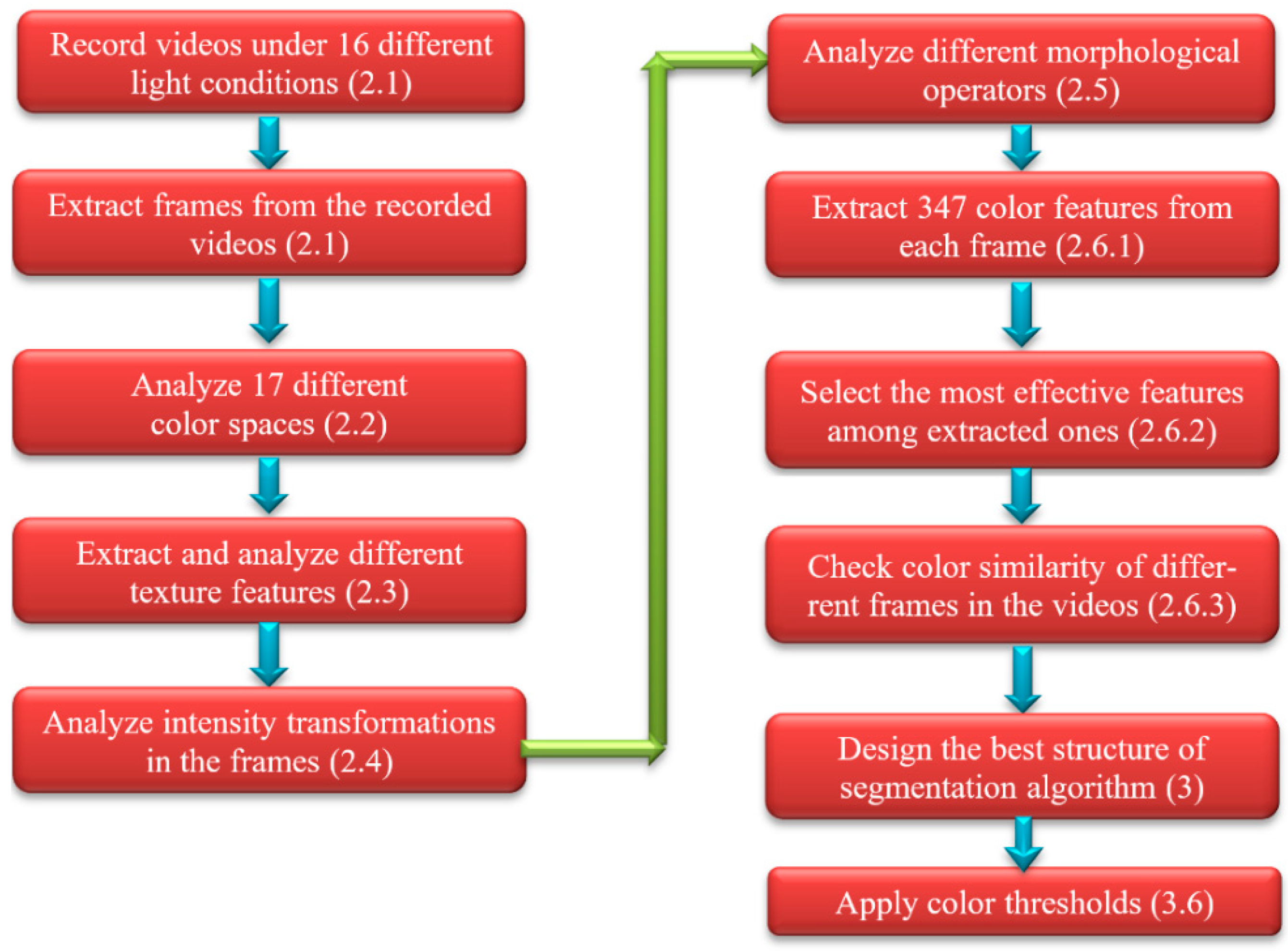
Funding

This research was funded by Iran National Science Foundation (INSF) through the research project 96007466, and by the Spanish MINECO, as well as European Commission FEDER funds, under grants numbers TIN2015-66972-C5-3-R and AGL2015-66938-C2-1-R.

Conflicts of Interest

The authors declare no conflict of interest. The funders had no role in the design of the study; in the collection, analyses, or interpretation of data; in the writing of the manuscript, and in the decision to publish the results.

References

  1. Slaughter, D.C.; Giles, D.K.; Downey, D. Autonomous robotic weed control systems: A review. Comput. Electron. Agric. 2008, 61, 63–78. [Google Scholar] [CrossRef]
  2. Lei, Z.; Jun, K.; Xiaoyun, Z.; Jiayue, R. Plant species identification based on neural network. In Proceedings of the 4th International Conference on Natural Computation, Jinan, China, 18–20 October 2008; pp. 90–94. [Google Scholar] [CrossRef]
  3. Kataoka, T.; Kaneko, T.; Okamoto, H.; Hata, S. Crop growth estimation system using machine vision. In Proceedings of the IEEE/ASME International Conference on Advanced Intelligent Mechatronics (AIM 2003), Kobe, Japan, 20–24 July 2003; pp. 1079–1083. [Google Scholar] [CrossRef]
  4. Camargo, A.; Smith, J.S. An image-processing based algorithm to automatically identify plant disease visual symptoms. Biosyst. Eng. 2009, 102, 9–21. [Google Scholar] [CrossRef]
  5. Hamuda, E.; Glavin, M.; Jones, E. A survey of image processing techniques for plant extraction and segmentation in the field. Comput. Electron. Agric. 2016, 125, 184–199. [Google Scholar] [CrossRef]
  6. Dorj, U.O.; Lee, M.; Yun, S.-S. An yield estimation in citrus orchards via fruit detection and counting using image processing. Comput. Electron. Agric. 2017, 140, 103–112. [Google Scholar] [CrossRef]
  7. Behroozi-Khazaei, N.; Maleki, M.R. A robust algorithm based on color features for grape cluster segmentation. Comput. Electron. Agric. 2017, 142, 41–49. [Google Scholar] [CrossRef]
  8. Hu, Q.-X.; Tian, J.; He, D.-J. Wheat leaf lesion color image segmentation with improved multichannel selection based on the Chan–Vese model. Comput. Electron. Agric. 2017, 135, 260–268. [Google Scholar] [CrossRef]
  9. Casanova, J.J.; O’Shaughnessy, S.A.; Evett, S.R.; Rush, C.M. Development of a wireless computer vision instrument to detect biotic stress in wheat. Sensors 2014, 14, 17753–17769. [Google Scholar] [CrossRef] [PubMed]
  10. Singh, V.; Misra, A.K. Detection of plant leaf diseases using image segmentation and soft computing techniques. Inf. Process. Agric. 2017, 4, 41–49. [Google Scholar] [CrossRef]
  11. Camino, C.; Zarco-Tejada, P.J.; Gonzalez-Dugo, V. Effects of heterogeneity within tree crowns on airborne-quantified SIF and the CWSI as indicators of water stress in the context of precision agriculture. Remote Sens. 2018, 10, 604. [Google Scholar] [CrossRef]
  12. Zhou, X.; Sun, J.; Mao, H.P.; Wu, X.H.; Zhang, X.D.; Yang, N. Visualization research of moisture content in leaf lettuce leaves based on WT-PLSR and hyperspectral imaging technology. J. Food Process Eng. 2018, 41, E12647. [Google Scholar] [CrossRef]
  13. Hernández-Hernández, J.L.; Ruiz-Hernández, J.; García-Mateos, G.; González-Esquiva, J.M.; Ruiz-Canales, A.; Molina-Martínez, J.M. A new portable application for automatic segmentation of plants in agriculture. Agric. Water Manag. 2017, 183, 146–157. [Google Scholar] [CrossRef]
  14. Li, Y.; Cao, Z.; Lu, H.; Xiao, Y.; Zhu, Y.; Cremers, A.B. In-field cotton detection via region-based semantic image segmentation. Comput. Electron. Agric. 2016, 127, 475–486. [Google Scholar] [CrossRef]
  15. García-Mateos, G.; Hernández-Hernández, J.L.; Escarabajal-Henarejos, D.; Jaén-Terrones, S.; Molina-Martínez, J.M. Study and comparison of color models for automatic image analysis in irrigation management applications. Agric. Water Manag. 2015, 151, 158–166. [Google Scholar] [CrossRef]
  16. Chaves-González, J.M.; Vega-Rodríguez, M.A.; Gómez-Pulido, J.A.; Sánchez-Pérez, J.M. Detecting skin in face recognition systems: A colour spaces study. Digit. Signal Process. 2010, 20, 806–823. [Google Scholar] [CrossRef]
  17. Chanwimaluang, T.; Fan, G. An efficient blood vessel detection algorithm for retinal images using local entropy thresholding. In Proceedings of the 2003 International Symposium on Circuits and Systems, Bangkok, Thailand, 25–28 May 2003. [Google Scholar]
  18. Haralick, R.M.; Sternberg, S.R.; Zhuang, X. Image analysis using mathematical morphology. IEEE Trans. Pattern Anal. Mach. Intell. 1987, PAMI-9, 532–550. [Google Scholar] [CrossRef]
  19. Gonzalez, R.C.; Woods, R.E.; Eddins, S.L. Digital Image Processing Using MATLAB; Prentice Hall: Upper Saddle River, NJ, USA, 2008; ISBN 9780070702622. [Google Scholar]
  20. Woebbecke, D.; Meyer, G.E.; Bargen, K.V.; Mortensen, D.A. Color indices for weed identification under various soil, residue, and lighting conditions. Trans. ASAE 1995, 38, 259–269. [Google Scholar] [CrossRef]
  21. Meyer, G.E.; Mehta, T.; Kocher, M.F.; Mortensen, D.A.; Samal, A. Textural imaging and discriminant analysis for distinguishing weeds for spot spraying. Trans. ASAE 1998, 41, 1189–1197. [Google Scholar] [CrossRef]
  22. Meyer, G.E.; Neto, J.A.C. Verification of color vegetation indices for automated crop imaging applications. Comput. Electron. Agric. 2008, 63, 282–293. [Google Scholar] [CrossRef]
  23. Woebbecke, D.M.; Meyer, G.E.; Bargen, K.V.; Mortensen, D.A. Plant species identification, size, and enumeration using machine vision techniques on near-binary images. Opt. Agric. For. 1992, 1836, 208–219. [Google Scholar] [CrossRef]
  24. Golzarian, M.R.; Frick, R.A. Classification of images of wheat, ryegrass and brome grass species at early growth stages using principal component analysis. Plant Methods 2011, 7, 7–28. [Google Scholar] [CrossRef] [PubMed]
  25. Mehmood, T.; Liland, K.H.; Snipen, L.; Sæbø, S. A review of variable selection methods in partial least squares regression. Chemometr. Intell. Lab. Syst. 2012, 118, 62–69. [Google Scholar] [CrossRef]
  26. Zameer, A.; Mirza, S.M.; Mirza, N.M. Core loading pattern optimization of a typical two-loop 300 MWe PWR using Simulated Annealing (SA), novel crossover Genetic Algorithms (GA) and hybrid GA(SA) schemes. Ann. Nucl. Energ. 2014, 65, 122–131. [Google Scholar] [CrossRef]
  27. Ali, M.Z.; Awad, N.H.; Suganthan, P.N.; Duwairi, R.M.; Reynolds, R.G. A novel hybrid Cultural Algorithms framework with trajectory-based search for global numerical optimization. Inform. Sci. 2016, 334, 219–249. [Google Scholar] [CrossRef]
  28. Sabzi, S.; Abbaspour-Gilandeh, Y.; García-Mateos, G. A new approach for visual identification of orange varieties using neural networks and metaheuristic algorithms. Inf. Process. Agric. 2017, 5, 162–172. [Google Scholar] [CrossRef]
  29. Wisaeng, K. A comparison of decision tree algorithms for UCI repository classification. Int. J. Eng. Trends Technol. 2013, 4, 3393–3397. [Google Scholar]
  30. Tang, J.-L.; Chen, X.-Q.; Miao, R.-H.; Wang, D. Weed detection using image processing under different illumination for site-specific areas spraying. Comput. Electron. Agric. 2016, 122, 103–111. [Google Scholar] [CrossRef]
  31. Aquino, A.; Diago, M.P.; Millan, B.; Tardaguila, J. A new methodology for estimating the grapevine-berry number per cluster using image analysis. Biosyst. Eng. 2017, 156, 80–95. [Google Scholar] [CrossRef]
Figure 1. Steps in the development of a complete algorithm for color segmentation of apples. In parentheses, a reference to the section/subsection where each step is described.
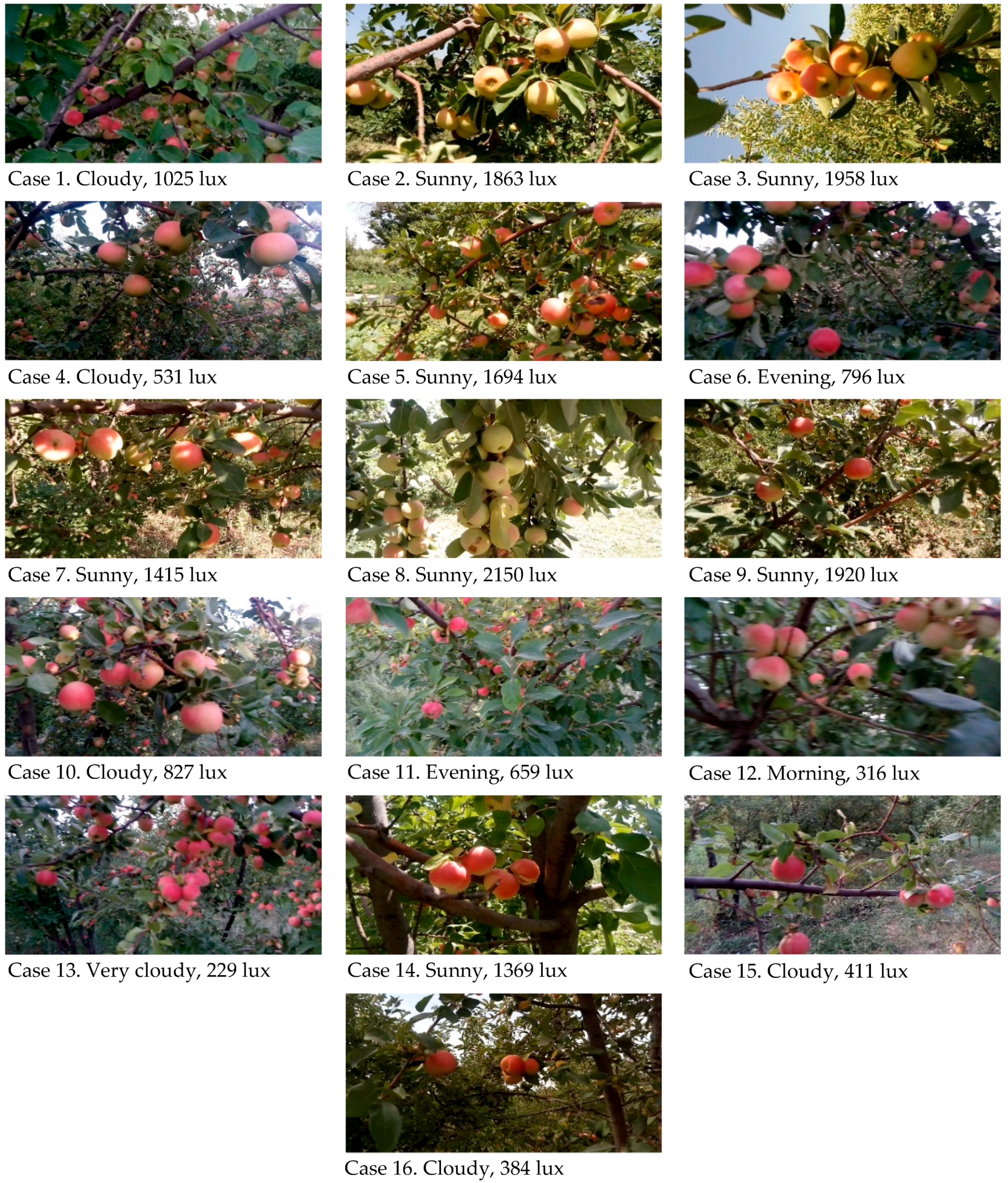
Water 10 01634 g001
Figure 2. Sample frames of videos taken under different lighting conditions. For each case, the weather condition and the measured light intensity (in lux) is indicated.
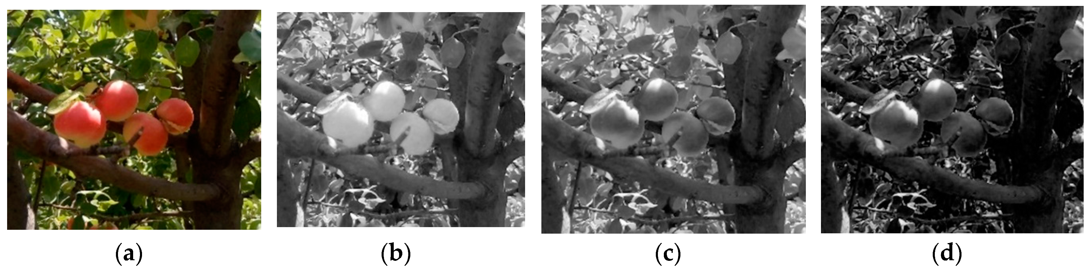
Water 10 01634 g002
Figure 3. Sample apple tree image and RGB channels. (a) Original RGB image. (b) R channel. (c) G channel. (d) B channel.
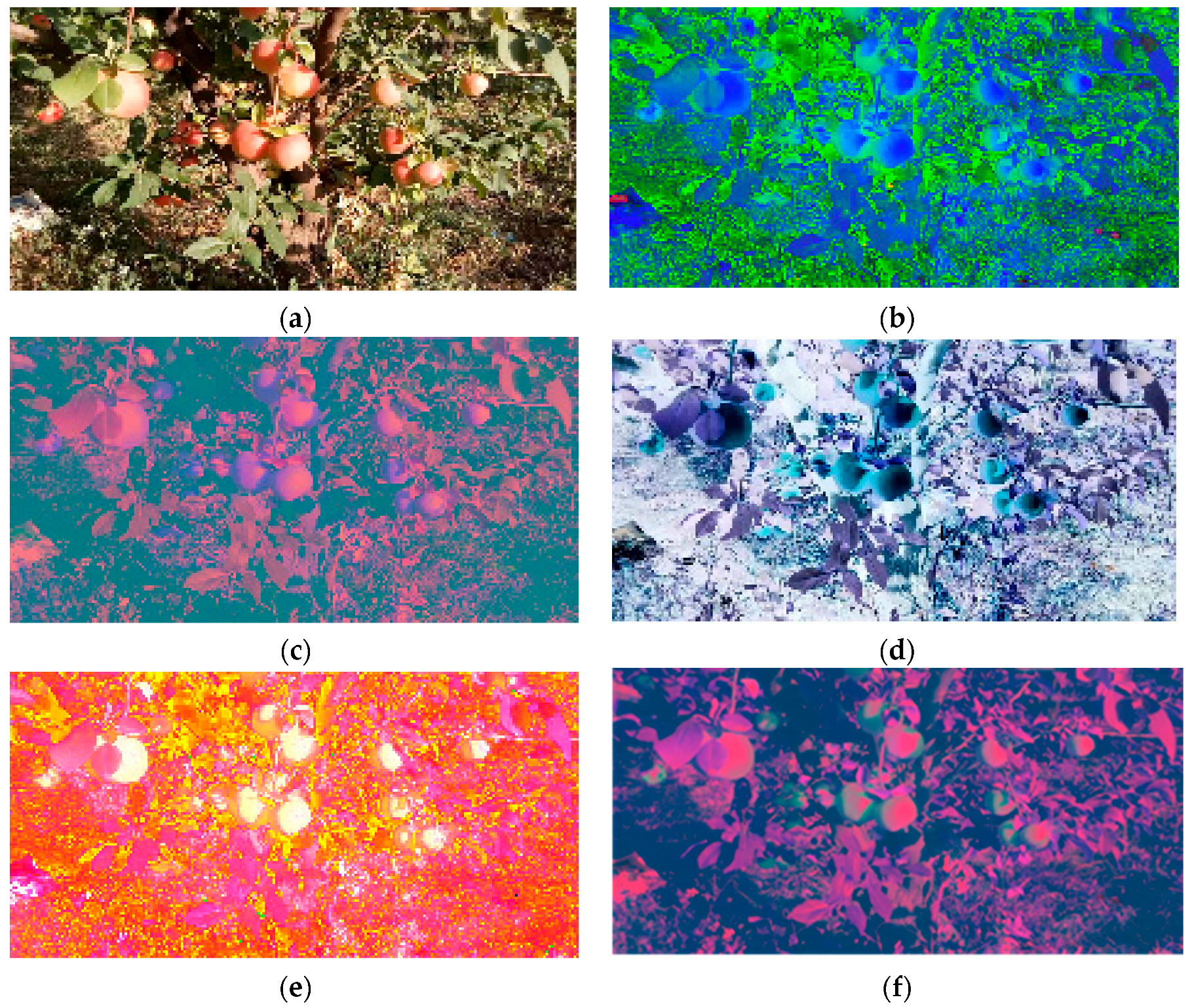
Water 10 01634 g003
Figure 4. Sample apple tree image under six different color spaces. (a) RGB color space. (b) HSV color space. (c) YCbCr color space. (d) CMY color space. (e) HSL color space. (f) L*u*v* color space. For visualization purposes, the three channels of each space are represented in the R, G, and B channels.
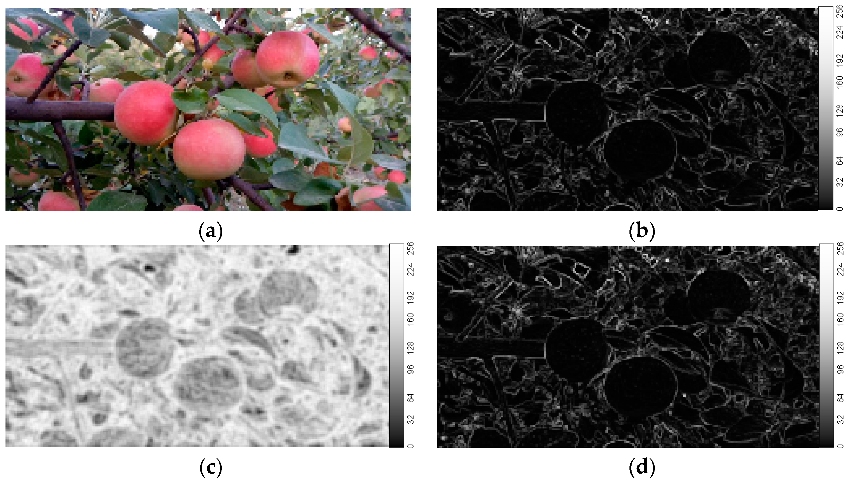
Water 10 01634 g004
Figure 5. Sample result of three texture features in an image of apples. (a) Original color image. (b) Image obtained by applying local range feature. (c) Local entropy feature. (d) Local standard deviation feature.
Water 10 01634 g005
Figure 6. Sample results of applying intensity segmentation on apple images. (a,d,g) Three color samples of the videos produced in 796, 1920, and 659 lux. (b,e,h) Results from the intensity transformation by selecting the R channel. (c,f,i) Segmentation images after applying the threshold.
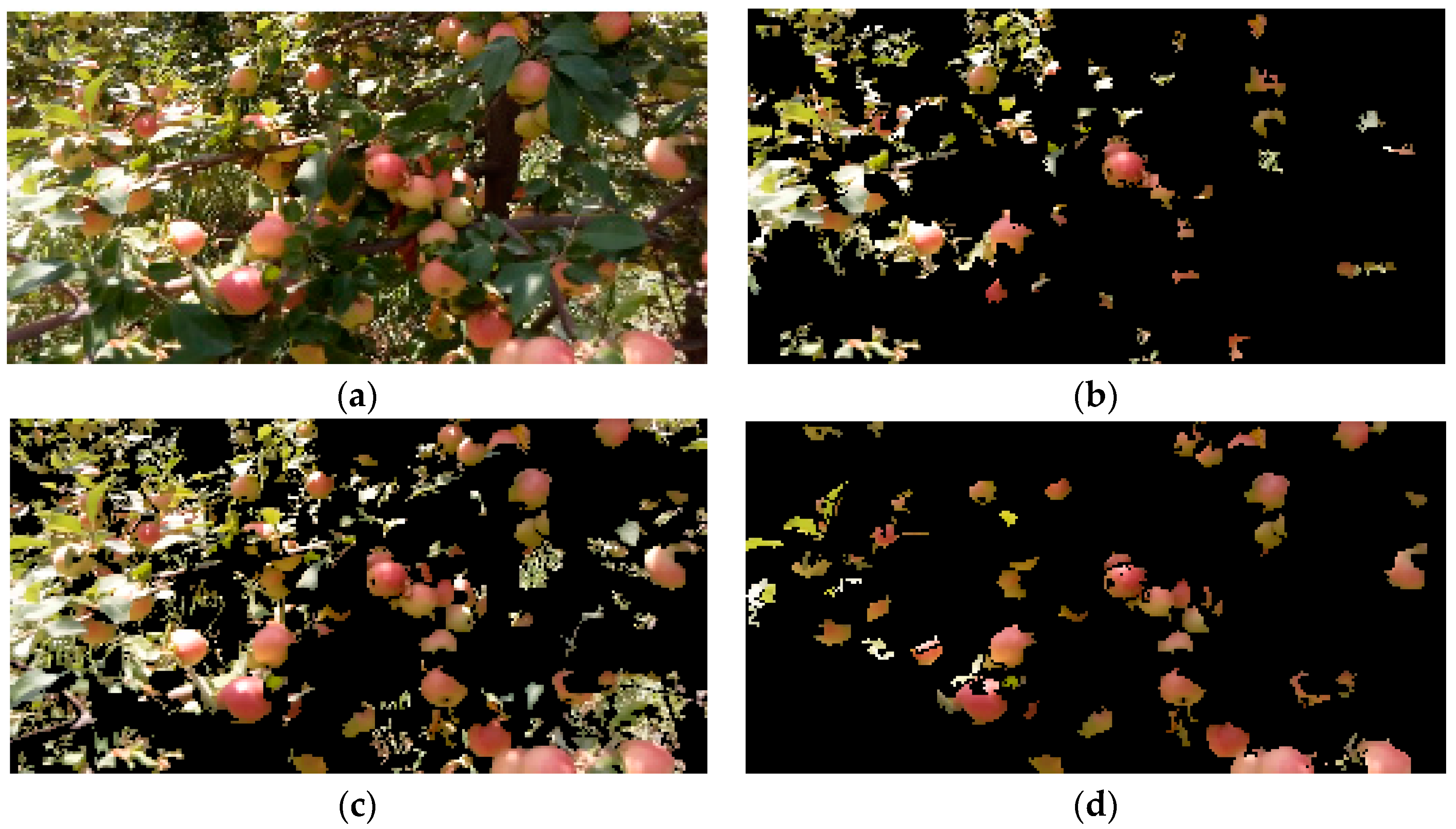
Water 10 01634 g006
Figure 7. Results of different orders of the color, texture and intensity steps on the segmentation algorithm. (a) Original color image of the apples. (b) Segmentation in texture, color and intensity order. (c) Segmentation in intensity, texture and color order. (d) Segmentation in color, texture, and intensity order.
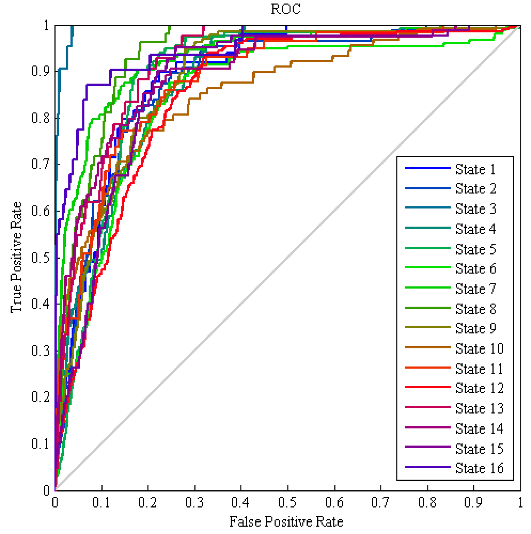
Water 10 01634 g007
Figure 8. Receiver operating characteristic (ROC) graph of the hybrid ANN-CA classification of frames for the 16 different classes, using color features.
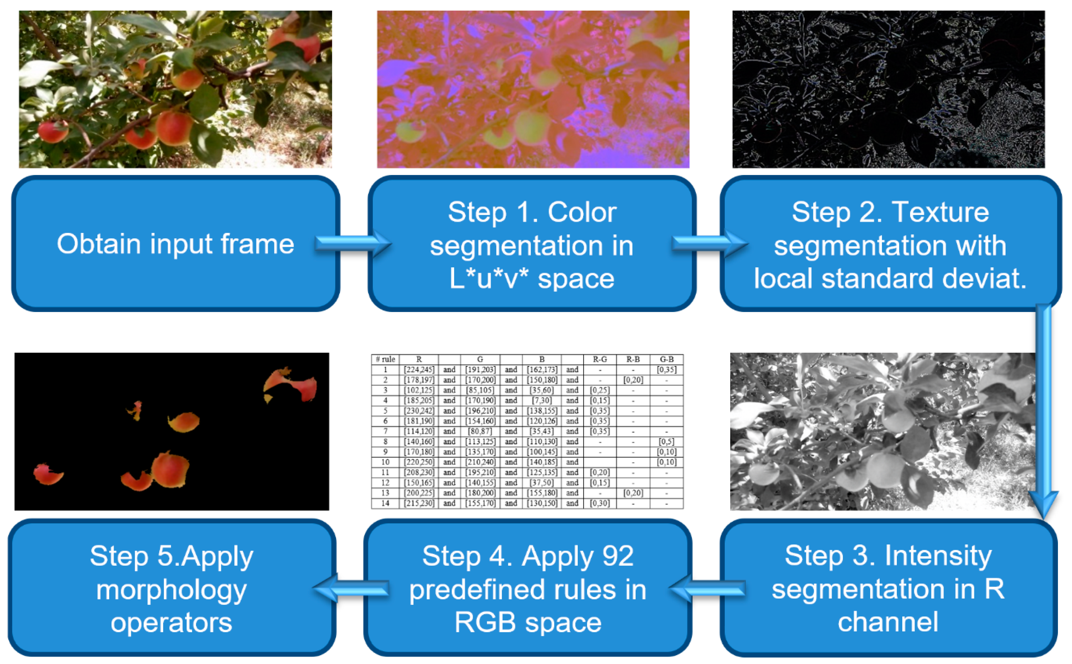
Water 10 01634 g008
Figure 9. Flowchart of the proposed apple segmentation algorithm.
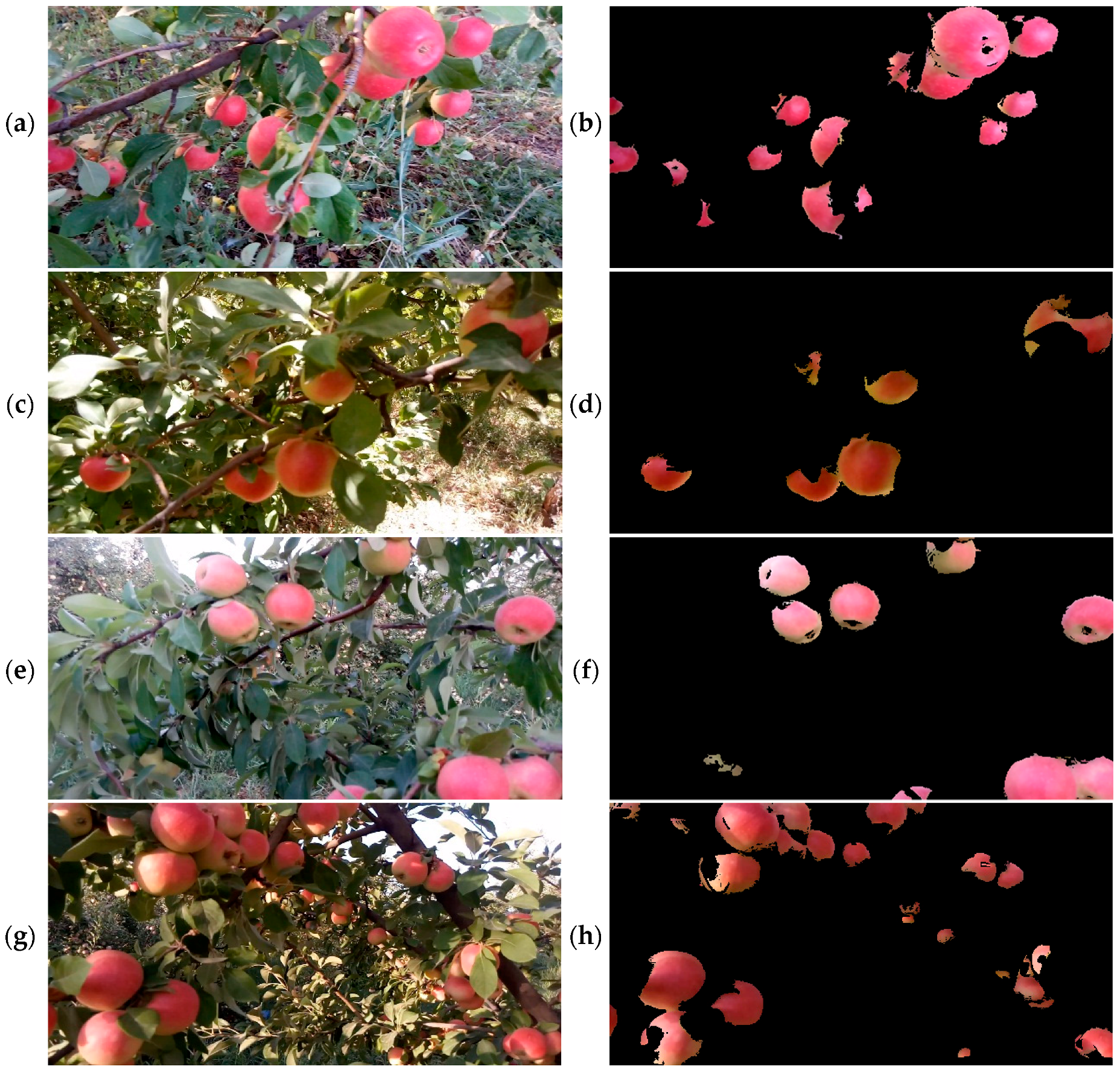
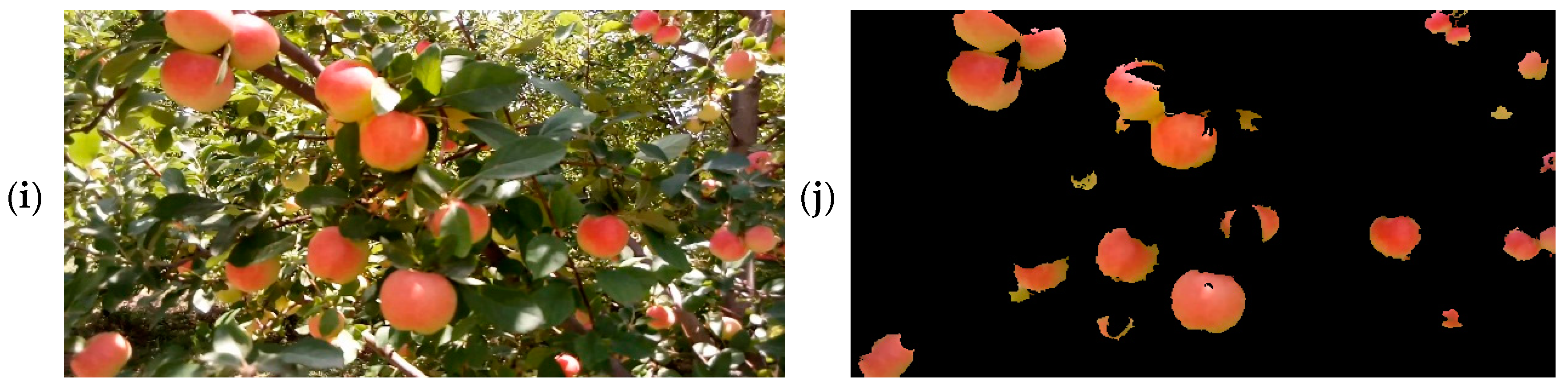
Water 10 01634 g009
Figure 10. Final segmentation results for five sample frames from different light intensities. (a,c,e,g,i) Original color images. (b,d,f,h,j) Corresponding segmented images, with background in black.
Water 10 01634 g010aWater 10 01634 g010b
Table 1. Characteristics of the videos captured under 16 different light conditions. The videos were obtained on different days. In the videos of evening and morning, the sky was clear.
Case NumberCapture DateWeather ConditionLight Intensity (lux)Time of the DayVideo Length (min)Total Number of FramesTrain/Test + Evaluation Frames
116 July 2017Cloudy102513:25 05:0518301281/549
217 July 2017Sunny186311:1010:0436242537/1087
320 July 2017Sunny195814:3001:03378265/113
423 July 2017Cloudy53115:3507:2526701869/801
525 July 2017Sunny169416:3610:1737022592/1110
629 July 2017Evening79618:0512:0943743062/1312
71 August 2017Sunny141510:1511:0539902793/1197
83 August 2017Sunny215013:1503:141164815/349
95 August 2017Sunny192012:0012:2544703129/1341
109 August 2017Cloudy82714:1007:2326581861/797
1110 August 2017Evening65919:1506:0021601512/648
1213 August 2017Morning31607:2518:0465044553/1952
1315 August 2017Very cloudy22920:0500:53318223/95
1418 August 2017Sunny136909:0506:3423641655/709
1520 August 2017Cloudy41116:2507:4627961957/838
1622 August 2017Cloudy38417:1502:32912639/274
Table 2. Color features extracted for each pixel, related to vegetation indices. Rn, Gn, and Bn refer to normalized red, green, and blue, respectively.
Extracted FeatureFormula for Calculating the Feature
Normalized first component of RGBRn = R/(R + G + B)
Normalized second component of RGBGn = G/(R + G + B)
Normalized third component of RGBBn = B/(R + G + B)
Gray channelgray = 0.2898 × R + 0.5870 × G + 0.1140 × B
Additional green [20]EXG = 2 × Gn − Rn − Bn
Additional red [21]EXR = 1.4 × Rn − Gn
Color index for extracted vegetation cover [3]CIVE = 0.441 × Rn − 0.811 × Gn + 0.385 × Bn + 18.78
Subtraction between additional green and additional red [22]EXGR = EXG − EXR
Normalized difference index [23]NDI = (Gn − Rn)/(Gn + Rn)
Green index minus blue [20]GB = (Gn − Bn)
Red-blue contrast [24]RBI = (Gn − Bn)/(Gn + Bn)
Green-red index [24]ERI = (Rn − Gn) × (Rn − Bn)
Additional green index [24]EGI = (Gn − Rn) × (Gn − Bn)
Additional blue index [24]EBI = (Bn − Gn) × (Bn − Rn)
Table 3. Parameters used in the multilayer perceptron neural network for the selection of the most effective color features.
ParameterValue
Number of layers2
Number of neuronsFirst layer: 8
Second layer: 12
Transfer functionsFirst layer: hyperbolic tangent sigmoid
Second layer: hyperbolic tangent sigmoid
Backpropagation network training functionScaled conjugate gradient
Backpropagation weight/bias learning functionHebb with decay weight learning
Table 4. Values of the multilayer perceptron artificial neural network parameters adjusted by the cultural algorithm (ANN-CA method).
ParameterValue
Number of hidden layers3
Number of neuronsFirst layer: 25
Second layer: 25
Third layer: 25
Transfer functionsFirst layer: hyperbolic tangent sigmoid
Second layer: hyperbolic tangent sigmoid
Third layer: hyperbolic tangent sigmoid
Backpropagation network training functionLevenberg–Marquardt
Backpropagation weight/bias learning functionLVQ1 weight learning
Table 5. Confusion matrix of the classification of 43,914 frames in the 16 classes corresponding to the different lighting conditions, using color features and the hybrid ANN-CA method. Rows: real classes. Columns: predicted classes. The percentage of color sharing of each class is defined as the percentage of frames of that class classified in a different class.
12345678910111213141516Color Sharing by Class (%)Total Color Sharing (%)
133000200052000090044000250081.9758.96
2018070013300901041320001002902003093.93
31802626001001024042006030.69
4110005100830000300071000210080.90
502321500171005030990000052002053.81
680001600231010002900130000224047.19
705020301601302750801408003600201304031.08
80126002404425861800120820075.29
902308001270017038019300000330305056.82
100007804701800401030074000120061.25
11001020012010900709005500201900100
122200307007703003001800433000574033.27
133001200418006501326024098.11
14030100710020805800024089002062.35
1530010900760200090086000936066.52
16010004001103072003010309049044.05
Table 6. Thresholds defined in RGB color space for the segmentation of background pixels.
Rule NumberR G B R-GR-BG-B
1[224,245]and[191,203]and[162,173]and--[0,35]
2[178,197]and[170,200]and[150,180]and-[0,20]-
3[102,125]and[85,105]and[35,60]and[0,25]--
4[185,205]and[170,190]and[7,30]and[0,15]--
5[230,242]and[196,210]and[138,155]and[0,35]--
6[181,190]and[154,160]and[120,126]and[0,35]--
7[114,120]and[80,87]and[35,43]and[0,35]--
8[140,160]and[113,125]and[110,130]and--[0,5]
9[170,180]and[135,170]and[100,145]and--[0,10]
10[220,250]and[210,240]and[140,185]and -[0,10]
11[208,230]and[195,210]and[125,135]and[0,20]--
12[150,165]and[140,155]and[37,50]and[0,15]--
13[200,225]and[180,200]and[155,180]and-[0,20]-
14[215,230]and[155,170]and[130,150]and[0,30]--
15[185,195]and[170,185]and[120,130]and[0,20]--
16[142,167]and[120,139]and[67,97]and[0,30]--
17[170,185]and[155,170]and[13,30]and[0,20]--
18[200,222]and[175,202]and[110,125]and[0,35]--
19[198,225]and[186,210]and[50,76]and-[0,20]-
20[178,182]and[164,167]and[126,133]and[0,18]--
21[98,116]and[70,98]and[50,83]and[0,30]--
22[129,140]and[110,120]and[109,120]and--[0,10]
23[239,255]and[230,255]and[55,170]and-[0,25]-
24[180,255]and[180,255]and[180,255]and---
25[160,200]and[149,180]and[30,60]and[0,20]--
26[200,220]and[190,210]and[120,145]and[0,15]--
27[125,140]and[117,130]and[25,42]and-[0,15]-
28[170,190]and[140,155]and[130,140]and--[0,20]
29[178,185]and[125,140]and[105,125]and--[0,25]
30[195,220]and[185,210]and[135,155]and[0,15]--
31[220,235]and[195,215]and[150,180]and[0,30]--
32[92,102]and[82,94]and[20,35]and[0,15]--
33[100,110]and[75,90]and[68,82]and--[0,15]
34[220,230]and[193,207]and[125,145]and[0,30]--
35[212,230]and[202,220]and[20,38]and[0,15]--
36[105,108]and[74,77]and[64,66]and--[0,15]
37[96,100]and[74,78]and[66,70]and[0,10]--
38[95,127]and[91,110]and[85,90]and[0,35]--
39[150,155]and[136,140]and[119,122]and--[0,20]
40[146,166]and[133,150]and[49,54]and[0,20]--
41[97,110]and[84,95]and[30,45]and[0,15]--
42[120,135]and[100,115]and[55,68]and[0,25]--
43[120,155]and[95,120]and[80,100]and--[0,25]
44[195,210]and[160,185]and[125,150]and[50,70]--
45[110,115]and[75,78]and[57,78]and--[0,20]
46[115,130]and[100,115]and[49,55]and[0,20]--
47[132,142]and[78,85]and[52,58]and--[0,30]
48[92,130]and[63,95]and[12,35]and[0,35]--
49[220,225]and[226,242]and[102,110]and-[0,20]-
50[127,142]and[96,110]and[68,77]and[0,35]--
51[120,140]and[85,110]and[50,67]and-[0,40]-
52[100,160]and[100,160]and[10,50]and[0,10]--
53[189,200]and[171,191]and[60,9]and[0,15]--
54[105,120]and[85,100]and[48,60]and[0,25]--
55[225,235]and[170,180]and[135,145]and--[0,35]
56[215,220]and[195,205]and[150,160]and[0,25]--
57[190,202]and[179,190]and[48,53]and[0,20]--
58[109,122]and[68,90]and[42,58]and--[0,35]
59[109,120]and[65,80]and[69,75]and-[0,35]-
60[129,140]and[89,95]and[64,75]and--[0,27]
61[191,195]and[170,178]and[128,132]and[0,25]--
62[155,170]and[132,152]and[100,125]and[0,35]--
63[95,105]and[57,72]and[27,42]and--[0,35]
64[110,135]and[90,120]and[85,110]and--[0,15]
65[250,255]and[182,188]and[146,149]and--[0,40]
66[215,220]and[183,190]and[135,140]and[0,35]--
67[113,122]and[87,93]and[81,87]and--[0,10]
68[227,242]and[211,225]and[72,82]and[0,20]--
69[164,172]and[150,159]and[95,105]and[0,20]--
70[139,145]and[111,120]and[70,81]and[0,35]--
71[142,152]and[118,127]and[90,107]and--[0,30]
72------[0,10]--
73[122,131]and[105,110]and[56,60]and[0,22]--
74[230,245]and[165,175]and[120,130]and--[35,50]
75[225,235]and[170,180]and[135,145]and-[0,40]-
76[90,110]and[55,80]and[40,62]and--[0,20]
77[195,207]and[179,182]and[25,33]and[0,27]--
78[244,248]and[232,236]and[84,88]and[0,15]--
79[181,189]and[169,178]and[113,121]and[0,15]--
80[190,210]and[180,205]and[110,125]and[0,20]--
81[190,210]and[160,180]and[140,170]and--[0,20]
82[212,220]and[193,205]and[125,148]and[0,25]--
83[98,108]and[82,90]and[22,38]and[0,25]--
84[202,227]and[185,215]and[35,40]and[0,20]--
85[215,237]and[215,227]and[45,65]and-[0,15]-
86[170,205]and[165,185]and[87,100]and[0,20]--
87[125,160]and[110,145]and[55,90]and[0,20]--
88[222,230]and[161,169]and[130,137]and--[0,35]
89[155,185]and[130,165]and[110,150]and--[0,20]
90[195,215]and[165,195]and[120,140]and[0,35]--
91[120,128]and[110,118]and[40,55]and[0,15]--
92[95,115]and[49,70]and[25,50]and--[0,25]
Table 7. Confusion matrix and accuracy of the proposed apple segmentation algorithm in the test set.
Predicted/Real ClassAppleBackgroundAll DataClassification Error by Class (%)Classification Accuracy (%)
Apple91,40679892,2040.86599.12
Background1052117,496118,5480.887
Table 8. Confusion matrix and accuracy of the segmentation algorithm using neural networks on the test set.
Predicted/Real ClassAppleBackgroundAll DataClassification Error by Class (%)Classification Accuracy (%)
Apple87,090511492,2045.5595.23
Background4932113,616118,5484.16
Table 9. Confusion matrix and accuracy of the segmentation algorithm using color histogram models on the testing set.
Predicted/Real ClassAppleBackgroundAll DataClassification Error by Class (%)Classification Accuracy (%)
Apple88,103410192,2044.4596.80
Background2645115,903118,5482.23
Table 10. Measures of sensitivity (Sens.), specificity (Spec.) and accuracy (Accur.) of the proposed segmentation algorithm and the two methods used for comparison: neural networks and color histogram models.
Proposed MethodNeural NetworksColor Histograms
ClassSens. (%)Spec. (%)Accur. (%)Sens. (%)Spec. (%)Accur. (%)Sens. (%)Spec. (%)Accur. (%)
Apple99.1398.8699.1294.4594.6495.2395.5597.0996.80
Background99.1199.3395.8495.6997.7796.58
Table 11. Comparison of the segmentation accuracy of the proposed algorithm with respect to other recent research works.
MethodNumber of Test SamplesAccuracy Rate (%)
Proposed method210,75299.12
ANN method210,75295.23
Color histograms method210,75296.8
Tang et al. [30]10092.5
Aquino et al. [31]15295.72

