A Study of the Influence of the Spatial Distribution of Rain Gauge Networks on Areal Average Rainfall Calculation

Abstract

Estimating the AAR (Areal Average Rainfall) is an essential process when determining the accurate amount of available water resources and building the input data which is integral to the Rainfall-Runoff Analysis. To estimate the AAR, using rain gauge networks that are spatially well distributed is ideal. In this study, the spatial characteristics of the rain gauge networks for the five major river basins in South Korea are considered and the amount of influence the spatial distribution has on the estimation of the AAR is evaluated. For this purpose, the estimation error for AAR is calculated for two cases. The first case (Analysis 1) compares the value of the estimation error of the AAR from two different basins where one has well distributed rain gauges while the other does not. The second case (Analysis 2) estimates the estimation error of two different rain gauge distributions for the same basin. The spatial characteristic of the rain gauge network is evaluated by using the NNI (Nearest Neighbour Index), while the Arithmetic Mean Method, Thiessen Method and the Estimation Theory are applied to calculate the AAR. From Analysis 1, we are able to prove that the estimation error of the AAR is relatively small in the basins with that have spatially well distributed rain gauge networks whereas the estimation error is relatively large when the spatial distribution of the rain gauge network is clustered. Also, results from Analysis 2 showed that not only is the spatial distribution of the rain gauge networks important, but that the density has a significant influence on accurately calculating the AAR. The results from this study can be applied towards the ideal establishment of the rain gauge networks.

1. Introduction

The spatial distribution of the rain gauge networks is relevant for soil development, plant distribution and water resources. To solve land and water management related problems at catchment scale, it is important to quantify and rainfall characteristic, water fluxes and associated substances [1,2]. The runoff analysis is highly determined by the rainfall distribution. Such hydrologic data can be obtained from hydrologic stations. Hydrological networks can largely be classified into water level observation networks, discharge observational networks and rain gauge networks. Of these three, evaluating the rain gauge networks is also essential to calculating both the accurate amount of available water resources and the AAR (Areal Average Rainfall), which is used as input data in the rainfall-runoff analysis [3]. If the appropriate rain gauge network cannot be secured, the error in the AAR estimation will create a significant error when simulating rainfall-runoff events [4]. Currently, the rain gauges are established and operated with the purpose of watching out for severe weather, flood forecast warning, maintaining and operating multipurpose dams. Rain gauge networks should be designed to provide a good estimate of AAR. The focus is placed on the estimation accuracy of AAR and estimation accuracies of point rainfall at individual ungauged sites are not of major concern [5]. These rain gauge networks, which are established for such specific purposes are evaluated by the entropy theory, principal component regression analysis, as well as correlation analysis [6,7,8,9,10]. While these methods evaluate the rain gauge networks based on the characteristics of the observed data, they do not take into consideration the spatial distribution of the rain gauge networks.

In general, rain gauge networks that are spatially well distributed have relatively small errors when calculating the AAR amount [11,12,13,14,15,16,17,18,19]. Therefore, for this purpose, the rain gauges should be spatially well distributed [9,20,21,22,23,24]. The previous studies on the effects of spatial distribution when calculating the AAR show the following. According to Dyck and Gray [3], rain gauge stations that are distributed evenly require less density than when they are distributed unevenly and that even when the number of rain gauges is reduced, the distribution of the rain gauge network is an important factor. Brock et al. [20] claim that when establishing the hydrological observation network, having a uniform distribution is most effective while Morrissey et al. [22] evaluated the importance of the distribution of the rain gauges using the standard error. Gracia et al. [21] evaluated the spatial distribution of the rain gauge stations using the clustering factor and Lee et al. [25] used the NNI (Nearest Neighbour Index) to evaluate the dispersion degree of the rain gauges. Furthermore, Hwang and Ham [26,27] evaluated the vulnerability of the rain gauges per area by using the observation density of each grid as well as the AAR. They also calculated the accuracy of the AAR on areas that lack density of rain gauge by using the PRISM (Parameter-elevation Regressions on Independent Slopes Model) method. Cheng et al. [5] evaluated and augmented rain gauge network using geostatistical approach and Barbalho et al. [28] compared the estimation techniques of AAR such as Thiessen polygon method, IDW (Inverse Distance Weighting), Kriging Method (KM), Multiquadric Equations Method (ME). According to Barbalho et al. [28], TM, IDW and ME Method are to be shown with good performance to obtain AAR. Whereas KM, tested with two variograms models, had a not expected unstable behaviour. True mean areal rainfall and its distributions will always remain unknown variable even various techniques of AAR estimation exist [28,29].

These previous studies show that uniform spatial distribution and dense rainfall station network are important to estimate more accurate AAR. This meaning is same that the design flood frequency increases as the design frequency rainfall increases. However, considering the economic aspect, the number of rainfall stations cannot be increased indefinitely. Therefore, for operation and maintenance, the rain gauge network should be quantified through considering the spatial distribution and the number of stations.

These studies show the significant effect of the spatial distribution of rain gauge stations when calculating the accurate AAR. However, there has yet to be research on calculating the AAR using actual rainfall event as well as the relationship between the spatial distribution and the AAR. Therefore, the purpose of this study is to analyse the spatial characteristics of the five major river basins of South Korea and to evaluate the influence of the rain gauge stations’ spatial distribution when calculating the AAR. The AAR is calculated using the arithmetic mean method, Thiessen method and the estimation theory while the spatial characteristic of a rain gauge network is evaluated using the NNI. The two basins are selected where one has a rain gauge network with rain gauge stations that are evenly distributed while the other network includes rain gauge stations that are not evenly distributed but clustered. The estimation error of the AAR is calculated for both of these basins and a smaller estimation error means a more accurate AAR (Analysis 1). However, the two sub-basins compared in Analysis 1 have different rainfall characteristics which affect the calculation of the AAR. To eliminate the effect from the differences of characteristics and to only consider the spatial distribution and density of the rain gauges when calculating the AAR, the number and distribution of the rain gauge stations are rearranged within the same basin (Analysis 2). Other methods for estimating the area mean rainfall are Kriging, IDW (Inverse Distance Weighting) and so on. However, these methods are excluded from this study because they complement the missing data or estimate the rainfall at ungauged point indirectly.

2. Theoretical Backgrounds

2.1. Nearest Neighbour Method

The spatial characteristic of a point can be evaluated by using the quadrat count method, nearest neighbour method, index of specialization as well as the index of localization. Most natural phenomena can be described by the Poisson distribution and it is used to describe the amount of times a rare event occurs within mostly the time, distance and specified region of space. If the points are randomly distributed, the shape of distribution will have areas where the points are both clustered as well as dispersed. When the shape does not have regularity like this, the Poisson distribution can be the standard to understanding it. Therefore, the Poisson distribution can be applied when the points are randomly distributed due to natural events [30,31].

The nearest neighbour method is applied when trying to understand the spatial characteristics of the point events. This method utilizes the spatial characteristics between any given point and its nearest points [32]. Since it calculates the distance between the two points and determines the spatial characteristics, it is considered to be a more geographical method than the quadrant method [33]. If the spatial distribution of points is clustered, the distances between the near points are smaller, while if it is dispersed the distance is bigger between the near points. Therefore, the ratio between the average of the nearest neighbour distance of the observed value and the expected average distance of the probability model can be used to calculate the distribution of the points and the clustering level. The dispersion and clustering level can be determined by first calculating the expected distance by applying the PDF and then comparing it to the average nearest distance of the observed data. This ratio is called the NNI (Nearest Neighbour Index) and can be expressed using the following:

$$\mathrm{NNI}=\frac{d_{obs}}{d_{exp}}$$

(1)

Here, $d_{obs}$ is the mean observed nearest neighbor distance and $d_{exp}$ is the mean expected nearest neighbour distance. Generally, if NNI = 1, it is the same as the assumed model, if $\mathrm{NNI}<1$, it means it is more clustered than the assumed model. Finally if $\mathrm{NNI}>1$, it means it is dispersed than the assumed model [32]. If it is assumed that all the points in the space follow the two dimensional Poisson distribution, the average distance between the nearest points will be $1/2\sqrt{\rho }$. Here, $\rho$ represents the density of the rain gauges (the number of rain gauges/study area). If the calculated distance using the observed data is smaller than the mean expected nearest neighbour distance, the points are clustered while larger means they are uniformly dispersed. If the points within the area are in a perfectly uniform pattern, this becomes an equidistant grid.

2.2. Calculation of the Estimation Error

Various techniques are often used to estimate AAR over an area such as arithmetic mean method, Thiessen method, IDW (Inverse Distance Weighting), Kriging method, isohyetal method, multiquadric equations method, estimation theory and so forth. The AAR estimation method can be classified into simple average estimation, method considered positional characteristics and method considered characteristics of data. Arithmetic mean method is very simple method to estimate AAR in great area. Thiessen method and isohyetal method are techniques for estimating the AAR based on the location of the rainfall station. Estimation theory considers the characteristics of the data to estimate the AAR.

On the other hand, IDW, Kriging method, multiquadric equations method are interpolation techniques for estimating the rainfall at ungauged stations. These techniques are mainly used for grid rainfall estimation to calibrate radar rainfall rather than estimate the AAR. The estimated value of IDW based on a weighting as a distance function is always constant. Kriging method based on regionalized variables concept consists of a set of techniques to estimate surfaces by modelling the spatial correlation structure of the variables. Whereas this method is known as a good interpolation technique, estimated value is different depending on Kriging type and how the variogram are assumed. The isohyetal method is useful because it reflects the mountain’s effect that cannot be detected in the Thiessen method, it is limited because the isohyet’s creation as well as establishment is subjective.

When estimation the grid rainfall by applying the IDW and the Kriging method, it becomes the uniformly distributed rainfall and their estimation error is equal to the arithmetic mean method. Furthermore, the grid rainfall is an estimated value and includes estimation errors. If the AAR is calculated with an estimation error included, a larger estimation error can be occurred. For this reasons, arithmetic mean method, Thiessen method and the estimation theory are applied to calculate AAR in this study.

The arithmetic mean method calculates the AAR by dividing the point rainfall observed by rain gauge stations in the basin by the total number of the stations. This can be used for a basin with uniformly distributed rain gauges. The Thiessen method assigns weight to each rainfall station in proportion to the Thiessen polygon area in case the rainfall stations are uniformly distributed. Another way to calculate the AAR is the estimation theory. The estimation theory, which has the advantage of being able to take into consideration the rainfall variability, uses the optimal weights to calculate the AAR amount [34,35,36]. AAR estimated by these methods includes the estimation error as shown in the following equation.

$$P_m=\widehat{{\mathrm{P}}_{\mathrm{m}}}+\mathsf{\epsilon }$$

(2)

Here, $P_m$ represents the AAR, $\widehat{{\mathrm{P}}_{\mathrm{m}}}$ is the estimated AAR calculated by the methods of AAR and $\mathsf{\epsilon }$ represents the estimation error when using these methods.

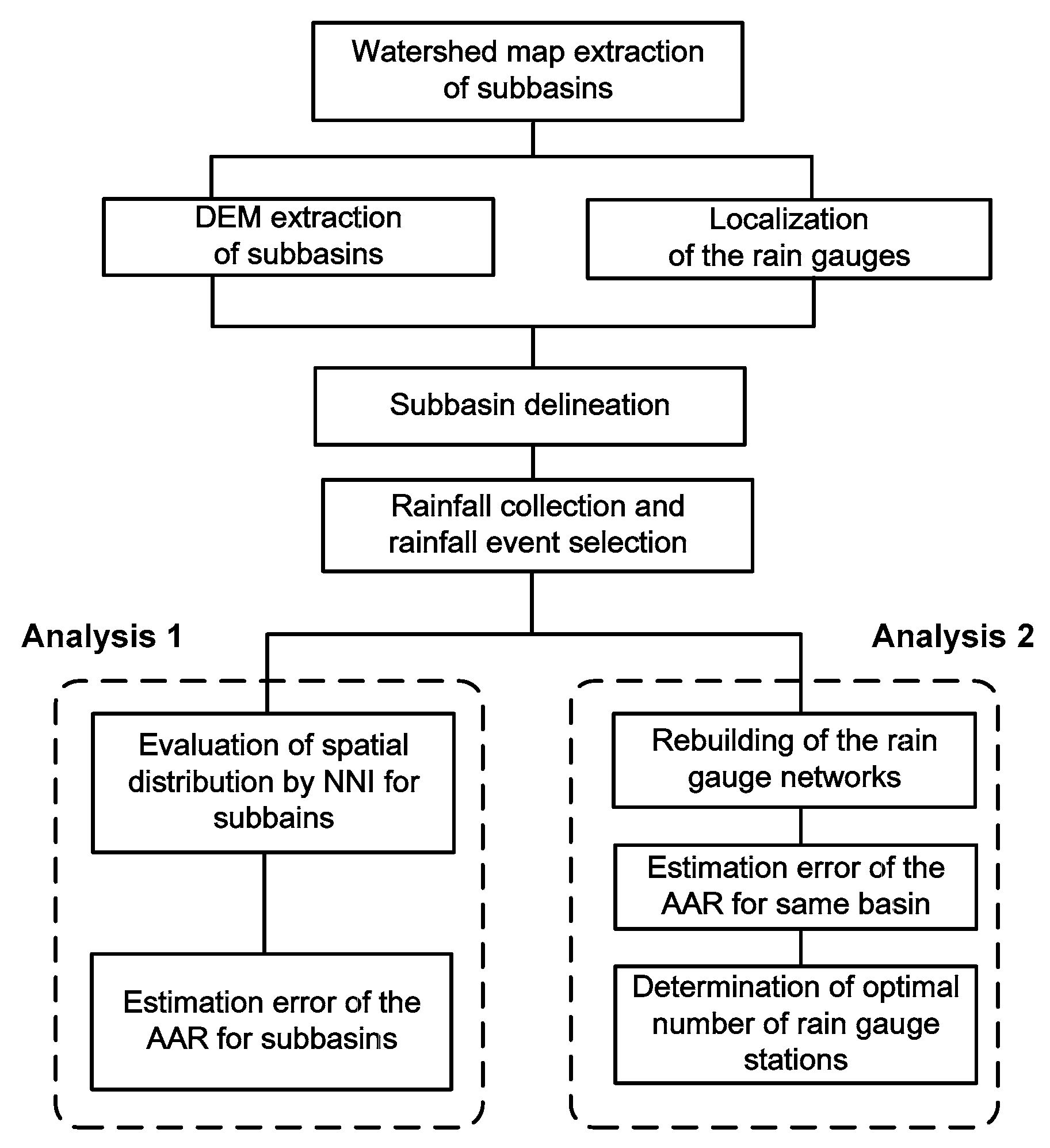
The arithmetic mean method assumes that the weight factor of each rain gauge station is the same and the estimation error is $\sqrt{\frac{{\sigma }^2}{n}}$. Here, $n$ represents the number of rain gauges, ${\sigma }^2$ is the average of variance in each rain gauge. The Thiessen method is based on the weights of the rain gauges computed by their relative areas, which are estimated with the Thiessen polygon network and the estimation error is $\sqrt{{\sum }_{k=1}^n{a}_k^2{\sigma }_k^2}$. Here, $a_k$ represents the area of Thiessen polygon and it can be calculated by dividing the relative area by basin area. If the rainfall stations in the area are uniformly dispersed, each $a_k$ will have a similar weighting factor and therefore will be close to the weighting factor used in the arithmetic mean method. Estimation theory has the advantage of considering the variability of rainfall. If there is a correlation between the rainfall stations, the observation error decreases. This can be analysed by using the EOF (Empirical Orthogonal Function) method and SVD (Singular Value Decomposition) method [37,38,39]. The estimation theory is based on the assumption that the rainfall stations are uniformly dispersed. This method uses the optimal weighting factor depending on the rainfall event and the estimation error is $\sqrt{\frac{1}{{\sum }_{k=1}^n\frac{1}{{\sigma }_k^2}}}$. The estimation methods of AAR and its estimation error are shown in

Table 1. Methodology of AAR and its Estimation Error.

AAR and Error	Arithmetic Mean Method	Thiessen Method	Estimation Theory
Estimated AAR ($\widehat{{\mathrm{P}}_{\mathrm{m}}}$)	$\frac{1}{\mathrm{n}}{\displaystyle {\displaystyle \sum }_{\mathrm{k}=1}^{\mathrm{n}}}{\mathrm{P}}_{\mathrm{k}}$	${\displaystyle {\displaystyle \sum }_{\mathrm{k}=1}^{\mathrm{n}}}{\mathrm{a}}_{\mathrm{k}}{\mathrm{P}}_{\mathrm{k}}$	$\frac{1}{{\mathsf{\eta }}^2}{\displaystyle {\displaystyle \sum }_{\mathrm{k}=1}^{\mathrm{n}}}\frac{{\mathrm{P}}_{\mathrm{k}}}{{\mathsf{\sigma }}_{\mathrm{k}}^2}\left({\mathsf{\eta }}^2={\displaystyle {\displaystyle \sum }_{\mathrm{k}=1}^n}\frac{1}{{\mathsf{\sigma }}_{\mathrm{k}}^2}\right)$
Estimation Error ($\mathsf{\epsilon }$)	$\sqrt{\frac{{\mathsf{\sigma }}^2}{\mathrm{n}}}$	$\sqrt{{\displaystyle {\displaystyle \sum }_{\mathrm{k}=1}^{\mathrm{n}}}{\mathrm{a}}_{\mathrm{k}}^2{\mathsf{\sigma }}_{\mathrm{k}}^2}$	$\sqrt{\frac{1}{{\sum }_{\mathrm{k}=1}^{\mathrm{n}}\frac{1}{{\mathsf{\sigma }}_{\mathrm{k}}^2}}}$

while Figure 1 illustrates the process of this study.

3. Study Area: 5 Major River Basins in Korea

3.1. Sub-Basin Delineation for Spatial Analysis

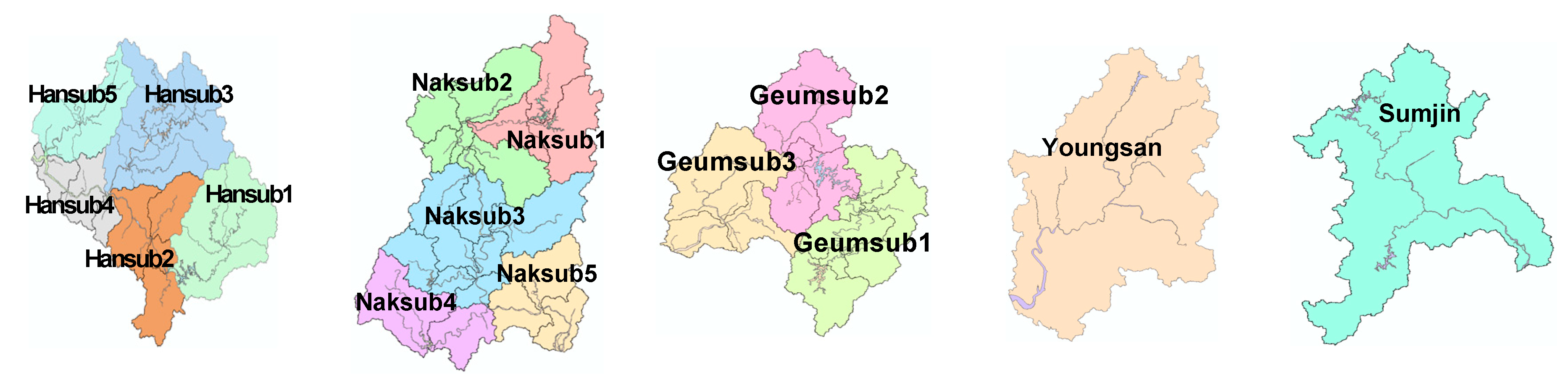
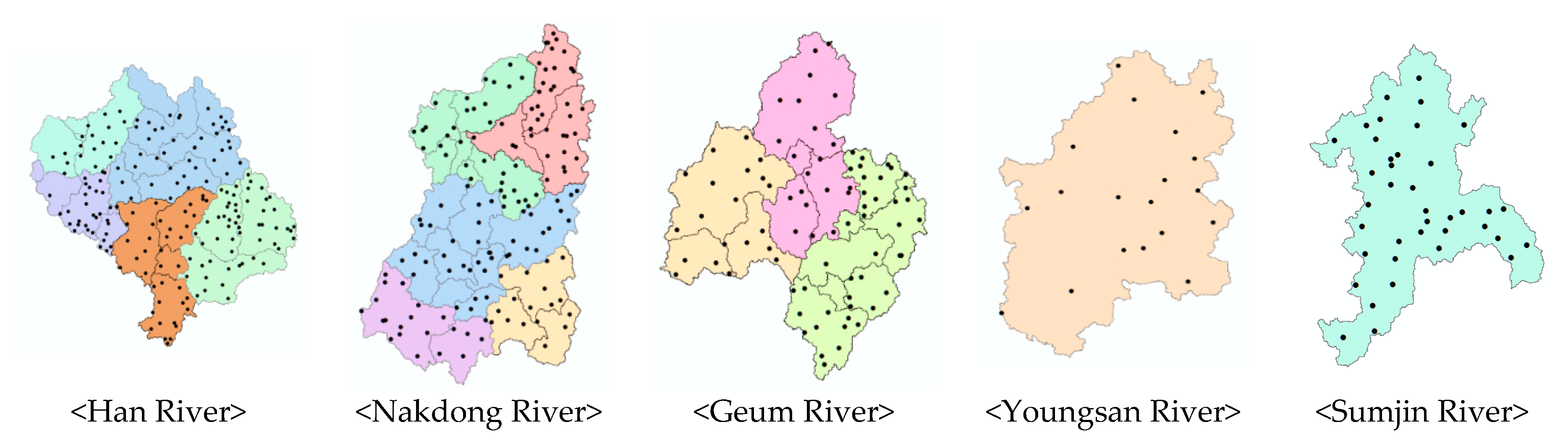
In this study, the Han River and Nakdong River basins are divided into five sub-basins while Keum River basin is divided into three sub-basins according to the watershed boundary and characteristics. Since the Yongsang River and Sumjin River basins have a small area, two river basins are assumed as each sub-basin. Each sub-basin of the five large river basins and the current rain gauges in each sub-basin are shown in Figure 2. Since the purpose of evaluating the spatial distribution of the rain gauges is to estimate the accurate AAR, this is done for each sub-basin.

3.2. Density of Rain Gauges in the Study Areas

When evaluating the rain gauge stations, whether a sufficient number of rain gauges have been established within the basin and whether they are appropriately established to satisfy the purpose of the rain gauge stations must first be considered. The density of rain gauge stations suggested by WMO (World Meteorological Organization) is used to determine whether there is a sufficient amount of rain gauges installed in the basin.

Table 2. Sub-basin Characteristics and the Density of Rain Gauges.

Five Large River Basins	Sub-basins	Area (km2)	# of Rain Gauges	Density
				(km2/# R.G.)	(# R.G./km2)
Han River	Hansub 1	6705.0	55	121.9	0.0082
	Hansub 2	5702.6	40	142.6	0.0070
	Hansub 3	7543.2	43	175.4	0.0057
	Hansub 4	3114.9	31	100.5	0.0100
	Hansub 5	3199.2	18	177.7	0.0056
Nakdong River	Naksub 1	4584.8	37	123.9	0.0081
	Naksub 2	4972.9	37	134.4	0.0074
	Naksub 3	7322.9	47	155.8	0.0064
	Naksub 4	3478.5	33	105.4	0.0095
	Naksub 5	3342.8	21	159.2	0.0063
Geum River	Geumsub 1	3566.2	41	87.0	0.0115
	Geumsub 2	3302.1	21	157.2	0.0064
	Geumsun 3	3046.7	20	152.3	0.0066
Youngsan River	Youngsan	3469.4	19	182.6	0.0055
Sumjin River	Sumjin	4914.3	39	126.0	0.0079
Sum/Ave.		68265.5	502	136.0	0.0074

shows the amount of rain gauge stations within each of the basins and its density.

There are a total 502 rain gauges established in all basins and the average density is 136.0 km²/rain gauge. The Geumsub 1 sub-basin has the highest density with 87.0 km²/rain gauge while the Youngsan sub-basin has the lowest with 182.6 km²/rain gauge.

Table 3. Recommended Minimum Densities of Stations (Area in per Station) [40].

Physiographic Unit	Precipitation
	Non-Recording	Recording
Coastal	900	9000
Mountains	250	2500
Interior plains	575	5750
Hilly/undulating	575	5750
Small islands	25	250
Polar/arid	10,000	100,000

shows the minimum densities of the stations depending on the rain gauge type suggested by the WMO [40].

The rain gauges of the study area are the recording type rain gauges and satisfy the minimum installation standard suggested by the WMO [40]. However, despite meeting the minimum installation standard, it is difficult to say whether the established rain gauges are uniformly dispersed. While the minimum density of the rain gauges suggested by the WMO makes it difficult to evaluate the spatial distribution characteristics but is the minimum standard for collecting rainfall data.

3.3. Evaluating the Spatial Characteristics of the Rain Gauge Network

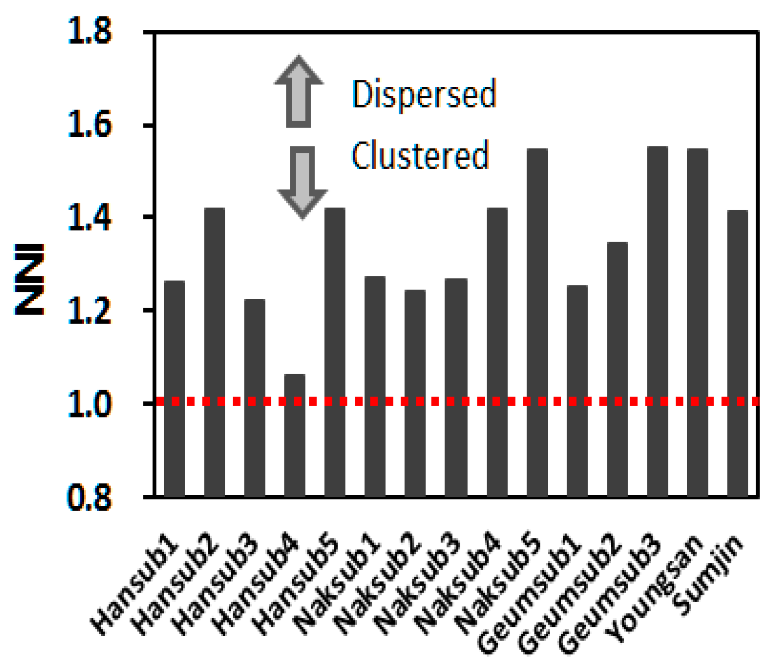
To evaluate the spatial characteristics of the rain gauges in each basin, the coordinates of rain gauges are collected. Using these coordinates, the distance between the rain gauges is calculated and finally the NNI for each sub-basin is estimated.

Table 4. Spatial Characteristics of the Rain Gauges for Each Sub-basin.

River Basins	Sub-basin	Expected Distance (km)	Observation Dist. (km)	NNI	Variance	Min. Observation Dist. (km)	Max. Observation Dist. (km)
Han River	Hansub 1	6.963	5.521	1.261	9.625	2.565	14.858
	Hansub 2	8.478	5.970	1.420	13.585	2.532	15.619
	Hansub 3	8.086	6.622	1.221	18.461	0.252	19.142
	Hansub 4	5.328	5.012	1.063	8.333	1.592	17.338
	Hansub 5	9.674	6.814	1.420	3.378	7.704	14.839
Nakdong River	Naksub 1	5.891	5.104	1.154	16.473	0.572	20.902
	Naksub 2	7.853	6.047	1.299	10.953	2.811	18.203
	Naksub 3	7.25	6.309	1.149	10.922	0.639	15.436
	Naksub 4	7.932	5.898	1.345	27.947	0.049	15.801
	Naksub 5	10.339	6.814	1.517	14.507	4.138	18.054
Geum River	Geumsub 1	5.848	4.663	1.254	7.065	0.736	13.468
	Geumsub 2	8.434	6.270	1.345	7.772	2.533	15.16
	Geumsub 3	9.563	6.171	1.550	9.757	4.639	15.228
Youngsan River	Youngsan	10.437	6.756	1.545	14.46	5.123	19.117
Sumjin River	Sumjin	7.943	5.613	1.415	10.188	2.589	18.664

shows the NNIs for each sub-basin.

Since the NNI is the larger than 1 in all of the sub-basins, the rain gauge stations are dispersed. Of all basins, the rain gauge of Geumsub 3 is the most dispersed with an NNI of 1.555 while the Hansub 4 is the most clustered with an NNI of 1.063. The minimum and maximum nearest neighbour distance of the Geumsub basin are 4.639 km and 15.228 km respectively, while the Hansub 4’s are 1.592 km and 17.338 km. The difference between the minimum and maximum nearest neighbour distance of the Geumsub 3 is smaller compared to the Hansub 4 which means that the distances between the rain gauges are uniform. Figure 3 compares the spatial characteristics of the rain gauges by sub-basins using the NNI.

As shown in Figure 4, it is evident that Geumsub 3 has rain gauges that are uniformly dispersed while Hansub 4 does not have any rain gauge stations established in certain areas while clustered in other areas.

4. Analysis of Estimation Error of the AAR

4.1. Selection of Rainfall Event for the Analysis

To evaluate the characteristics of the spatial distribution of the rain gauges by each sub-basin, the estimation error of the AAR for the basins with the best spatial distribution (Geumsub 3) and the worst (Hansub 4) are estimated. For water resources plan, AAR estimates of long-term rainfall, such as daily, monthly and annual rainfall, are needed. However, for the purpose of flood mitigation, hourly rainfall is often required and measurements of hourly or even smaller duration rainfalls are necessary [5]. According to Cheng et al. [5], hourly rainfall exhibits higher variability in space and the spatial variation structures among different storm types, whereas annual rainfall is shown to exhibit a less spatial variability. In this study, AAR is not calculated for each type of rainfall because the rain gauge network should be considered the water resources planning and flood mitigation. However, radar correction is mainly aimed at predicting extreme rainfall, so it should be reviewed for each type of rainfall. To calculate the estimation error of the AAR, we collected the observed hourly rainfall data occurred (April 2005 to August 2014) in those basins. The applied rainfall data are converted to digital signals by the telemetering system at the rainfall station and transmitted to the data processing centre by the wireless communication network in real time.

While the IETD (Inter Event Time Duration) used to separate the rainfall events is 12 h by assuming they are all natural watersheds, of the selected only the rainfall events that have a total rainfall amount of at least 30 mm and 5 h of rainfall duration are used. Using this as the standard, there are 87 rainfall events in the Geumsub 3 and 102 in the Hansub 4 as shown in

Table 5. Characteristic of the Observed Rainfall Events.

Sub-basin	Total Rainfall (mm)	Duration Time (h)	Total 5-Day Antecedent Rainfall (mm)	Maximum Rainfall Intensity (mm/h)	Average Rainfall Intensity (mm/h)
Geumsub 3 (87 events)	30.1–191.4 (59.4)	12–134 (54.1)	0.0–128.2 (20.4)	2.3–22.0 (8.9)	0.1–4.5 (1.3)
Hansub 4 (107 events)	30.1–469.9 (84.4)	10–122 (51.3)	0.0–460.9 (37.8)	1.7–35.6 (11.7)	0.3–6.8 (1.8)
			Minimum–Maximum (Average)

.

4.2. Estimation Error of the AAR by Comparison of Sub-basins (Analysis 1)

By applying rainfall events that have been selected, the estimation error of the AAR is calculated for Geumsub 3 and Hansub 4 by the arithmetic mean method, Thiessen method and estimation theory. The basin area of the Geumsub 3 is 3046.7 km² with 20 stations while Hansub 4 has a basin area of 3114.9 7 km² with 31 stations (See Table 2).

Table 6. Weighting Factor of Each Rain Gauge Station Depending on the Estimation Method of AAR.

Geumsub 3				Hansub 4
Station		Methods of Area Average Rainfall		Station		Methods of Area Average Rainfall		Station		Methods of Area Average Rainfall
#	Name	Arithmetic Mean	Thiessen	#	Name	Arithmetic Mean	Thiessen	#	Name	Arithmetic Mean	Thiessen
1	Ganggyeong	0.050	0.061	1	Kyoung An	0.032	0.052	21	Anyang	0.032	0.023
2	Gongju	0.050	0.050	2	Gwacheon	0.032	0.026	22	Yongin	0.032	0.009
3	Guam	0.050	0.088	3	Gwangju	0.032	0.025	23	Ui	0.032	0.051
4	Mireuksan	0.050	0.028	4	KoiSan	0.032	0.044	24	Unhak	0.032	0.009
5	Banpo	0.050	0.052	5	Guro	0.032	0.060	25	Uijeongbu	0.032	0.049
6	Bangdong	0.050	0.028	6	Gumi	0.032	0.029	26	Indukwon	0.032	0.010
7	Bokryong	0.050	0.082	7	Gunpo	0.032	0.013	27	Jangam	0.032	0.036
8	Yangchon	0.050	0.025	8	Geumgok	0.032	0.038	28	Jinjeop	0.032	0.032
9	Yeonsan	0.050	0.043	9	Gimpo	0.032	0.174	29	Toegyewon	0.032	0.023
10	Yugu	0.050	0.065	10	Naksaeng	0.032	0.017	30	Paldang dam	0.032	0.031
11	Eunjin	0.050	0.051	11	Namgok	0.032	0.016	31	Pogok	0.032	0.018
12	Janggi	0.050	0.038	12	Namhan sanseong	0.032	0.027
13	Jangseon	0.050	0.068	13	Naeri	0.032	0.015
14	Jeongsan	0.050	0.041	14	Naeri2	0.032	0.008
15	Jeongan	0.050	0.045	15	Daejang	0.032	0.015
16	Cheongyang	0.050	0.055	16	Mohyeon	0.032	0.043
17	Hagueon	0.050	0.023	17	Sanseong	0.032	0.018
18	Hansan	0.050	0.060	18	Sanggye	0.032	0.015
19	Hamyeol	0.050	0.038	19	Seongnam	0.032	0.024
20	Hongsan	0.050	0.058	20	Songjeong	0.032	0.051
Ave.		0.050	0.050	Ave.						0.032	0.038
Stdev.		0.000	0.018	Stdev.						0.000	0.039
Coeff. of variation		0.000	0.359	Coeff. of variation						0.000	1.050

below compares the weighting factors for the arithmetic mean method and the Thiessen method. In the case of the estimation theory, the weighting factor differs for each of the rain gauge stations depending on the rainfall events. However, for the arithmetic mean method and the Thiessen method, the weighting factors are the same for each of the stations for all rainfall events. The coefficient of variation of the Thiessen weighting factor for the Geumsub 3 is 0.359 which is 1.050 less than the Hansub 4. This means that when calculating the AAR by the Thiessen method, the Thiessen weighting factor of each of the rain gauge stations for the Geumsub 3 is relatively consistent and therefore the area of the corresponding Thiessen polygon is consistent. Since the arithmetic method applies an equal weight factor to each of the rain gauge stations, the coefficient of variation will be 0. In cases such as the Geumsub 3 where the spatial distribution of the rain gauges is uniformly distributed, the weighting factor for each of the rain gauge stations for the arithmetic mean method and the Thiessen method will be similar. The AAR calculated from the arithmetic mean method and the Thiessen method are very similar. This is due to the weighting factor used in both methods being similar.

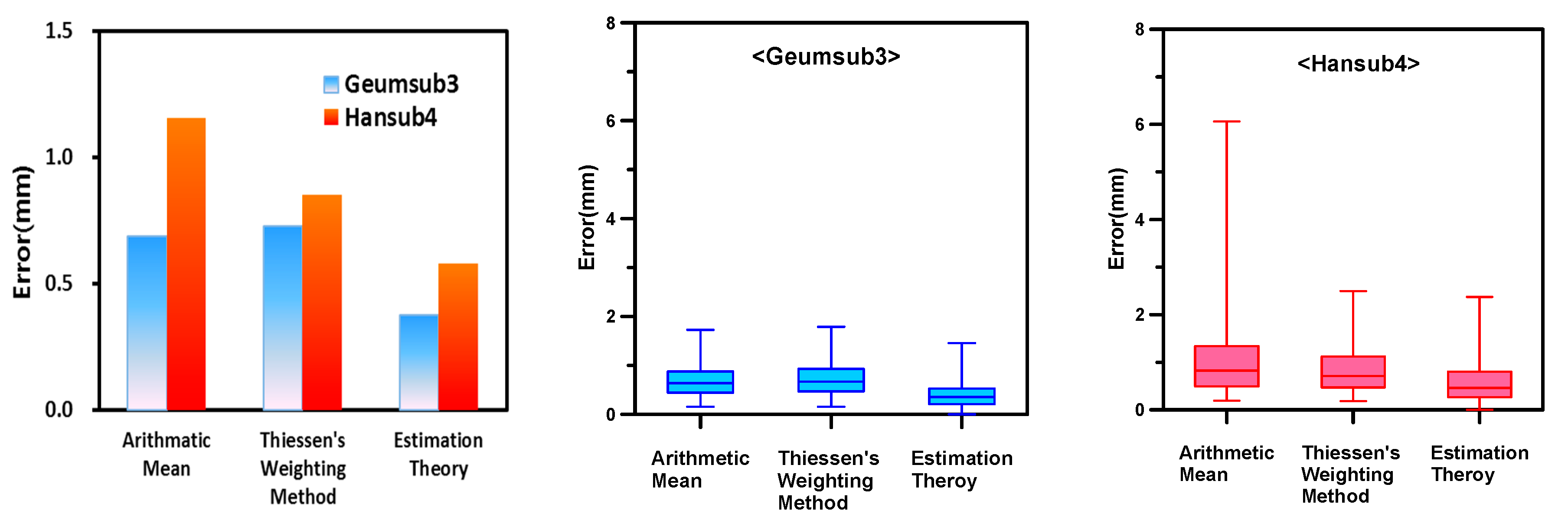
The results of calculating the statistical parameters of the AAR using the arithmetic mean method, Thiessen method and estimation theory are shown in

Table 7. Results of the Estimation Error Analysis Depending on the Estimation Method of AAR.

Statistics	Geumsub 3 (87 Events)			Hansub 4 (102 Events)
	Arithmetic Mean	Thiessen	Estimation Theory	Arithmetic Mean	Thiessen	Estimation Theory
Average	0.688	0.728	0.377	1.153	0.849	0.578
Standard Deviation	0.338	0.352	0.280	1.037	0.502	0.435
Coefficient of Variation	0.492	0.484	0.741	0.900	0.591	0.753

. When comparing the estimation error calculated from the two basins, the Geumsub 3 is smaller compared to the Hansub 4 (See Figure 5). The rain gauge stations in the Geumsub 3 have low spatial variability and therefore when calculating the AAR, the estimation error is small. Generally, the arithmetic mean method is good for a basin with the size of less than 500 km² while the Thiessen method is good for a basin of 500~5000 km² (Chow, 1988). However, if a basin whose area is larger than 500 km² has a rain gauge network with good spatial distribution, the arithmetic mean method can be used. It should also be noted that in cases where the spatial distribution is clustered, such as Hansub 4, using the arithmetic mean method could produce a large error which makes accurately calculating the AAR difficult. This is due to the fact that when the rain gauges are not uniformly dispersed, the fundamental assumption in the arithmetic mean method that each station is in equal corresponding area cannot be satisfied.

In addition, despite Hansub 4 having a higher density of rain gauges compared to Geumsub 3, a larger error is produced when calculating the AAR. This fact signifies that when calculating the AAR, not only is the density crucial but the spatial distribution is as well. However, in the case of Analysis 1 which compares each of the watersheds, the estimation error can differ depending on the geographical features and the characteristics of the observed rainfall data. To eliminate these effects and to explore only the effect that the spatial distribution and density of rain gauges have on calculating the AAR accurately, the number and distribution of the rain gauge stations are rearranged within the same basin and the same observed rainfall data (Analysis 2).

4.3. The estimation Error in the AAR for the same sub-basin (Analysis 2)

4.3.1. Rebuilding the Rain Gauge Networks

In this chapter, to estimate the effect of the geographical features and the characteristics of the observed rainfall data, a test basin is selected, and the estimation error of the AAR is estimated with different spatial distributions of rain gauge stations using the same observed rainfall events. The Geumsub 3, which is spatially well distributed, is selected as the test basin while the rain gauge networks are rearranged to calculate the AAR as well as the estimation error of it.

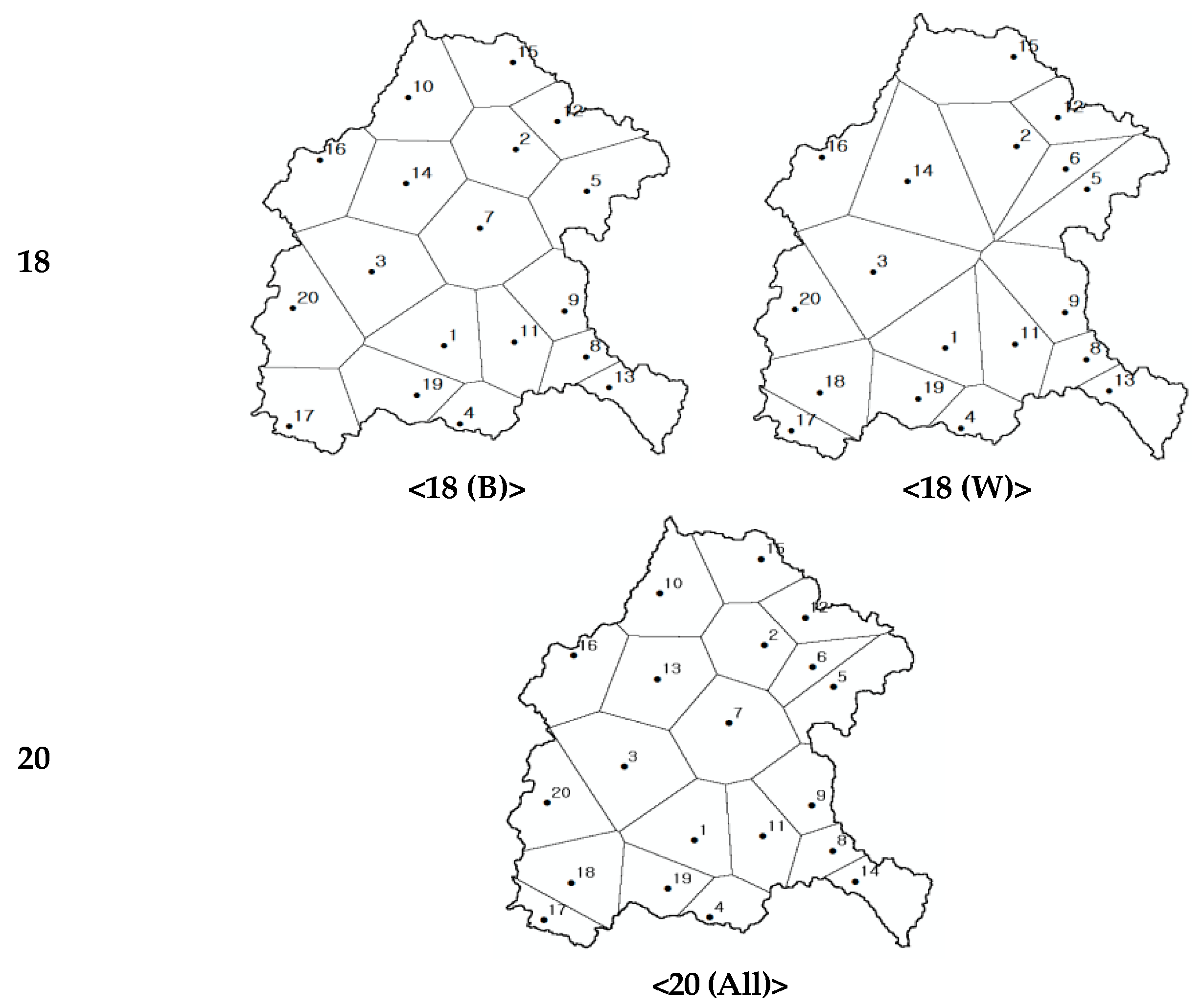
There are 20 rain gauges within Geumsub 3. 10 that are spatially well distributed are selected and labelled as 10 (B) while the others, which are not well distributed, are labelled as 10 (W). The AAR is then calculated using this newly formed rain gauge network. The same process is repeated but with 13, 15 and 18 station cases. The results are shown in

Table 8. The Number of the Possible Combinations of the Selected Stations Out of 20 Stations.

The Number of Selected Stations	Equation	The Number of the Combinations of the Stations
10	10C20	184,756
13	13C20	77,520
15	15C20	15,504
18	18C20	190

.

Table 9. Spatial distribution Depending on the Number of Rain Gauge Stations.

Case	Number of Rain Gauge Stations	NNI	Expected Distance (km)	Observation Distance (km)	Selected Combination of Rain Gauge Stations	Note
10 (B)	10	2.12	18.52	8.73	1, 4, 5, 7, 9, 13, 15, 16, 17, 20	Best spatial distribution of 10 rain gauge
10 (W)		0.80	6.97	8.73	2, 4, 5, 6, 8, 12, 13, 17, 18, 19	Worst spatial distribution of 10 rain gauge
13 (B)	13	1.97	15.11	7.65	2, 3, 4, 5, 7, 9, 10, 13, 14, 15, 16, 17, 20	Best spatial distribution of when 13 rain gauge
13 (W)		0.98	7.473	7.65	1, 2, 4, 5, 6, 8, 9, 11, 12, 13, 17, 18, 19	Worst spatial distribution of 13 rain gauge
15 (B)	15	1.88	13.42	7.13	1, 2, 3, 4, 5, 7, 9, 10, 12, 13, 14, 15, 16, 17, 20	Best spatial distribution of 15 rain gauge
15 (W)		1.16	8.25	7.13	1, 2, 4, 5, 6, 8, 9, 11, 12, 13, 14, 16, 17, 18, 19	Worst spatial distribution of 15 rain gauge
18 (B)	18	1.70	11.03	6.51	1, 2, 3, 4, 5, 7, 8, 9, 10, 11, 12, 13, 14, 15, 16, 17, 19, 20	Best spatial distribution of 18 rain gauge
18 (W)		1.39	9.04	6.51	1 ,2 ,3, 4, 5, 6, 8, 9, 11, 12, 13, 14, 15, 16, 17, 18, 19, 20	Worst spatial distribution of 18 rain gauge
20 (All)	20	1.55	9.56	6.17	All	All rain gauge applied

shows the NNIs calculated by the different cases of rain gauge networks and the condition of each case (“Note” in Table 8). Figure 6 shows the rain gauge networks of each case. To find the best and the worst spatial distribution of each case, we rely on the optimization algorithm with the harmony search method. In addition, 20 (All) represents the current rain gauges in the basin.

4.3.2. Rain Gauge Network Estimation Error Analysis

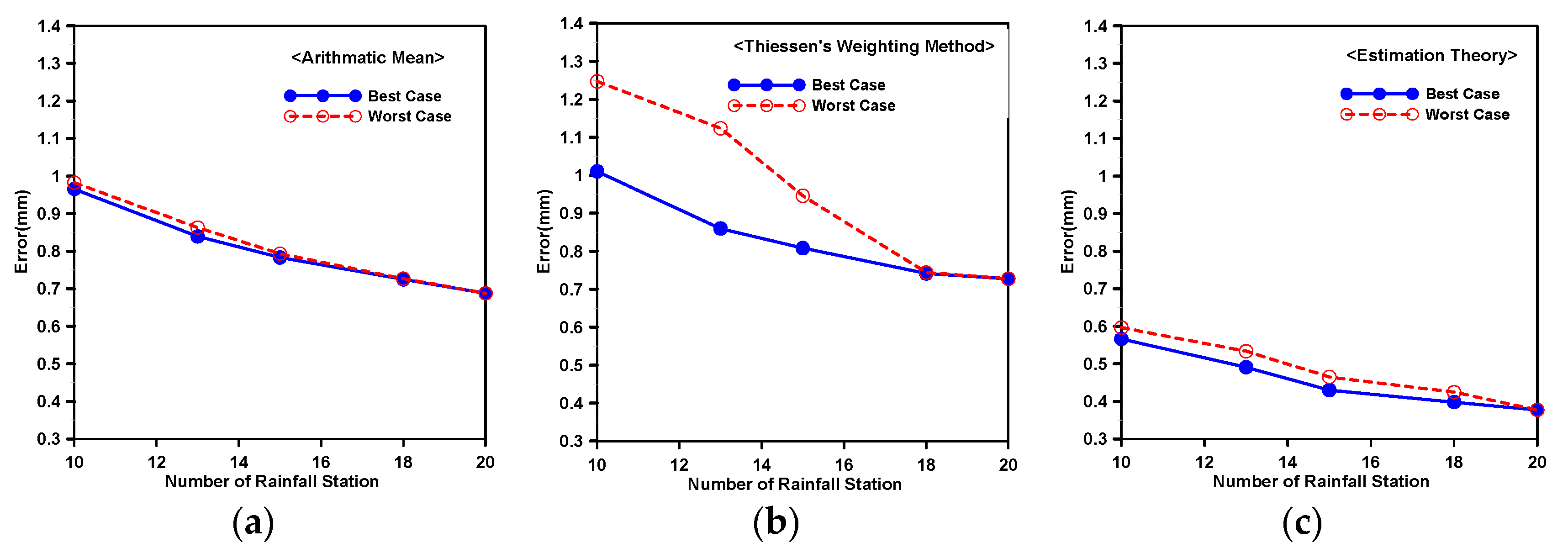
The same 87 rainfall events which were used to calculate the AAR in chapter 4.1 were applied for this analysis.

Table 10. Basic statistics of Thiessen Weighting Factors for AAR Estimation.

Cases	Average of Weighting Factor	Standard Deviation of Weighting Factor	CV of Weighting Factor
10 (B)	0.100	0.029	0.289
10 (W)	0.100	0.072	0.724
13 (B)	0.077	0.018	0.240
13 (W)	0.077	0.071	0.918
15 (B)	0.067	0.017	0.256
15 (W)	0.067	0.040	0.597
18 (B)	0.056	0.016	0.292
18 (W)	0.056	0.017	0.306
20 (All)	0.050	0.018	0.359

shows the basic statistics of the Thiessen weighting factors of each case. For all cases, if the number of rain gauges is same, the CV of Thiessen weighting factor at a well distributed network is smaller than that of the clustered network. This is due to the areas of Thiessen polygon becoming more constant as the spatial distribution of the rain gauge becomes well distributed. The NNI is calculated after the rain gauge networks are relocated according to the number of rain gauges. The estimation error of the AAR for the 87 rainfall events is calculated by applying the arithmetic method, Thiessen method and the estimation theory.

Table 11. Results of the Estimation Error Analysis by Rearranging the Rain Gauge Networks.

Case	Density (#/km2)	Density (km2/#)	NNI	Estimation Error
				Arithmetic Mean	Thiessen Method	Estimation Theory
10 (B)	0.0033	304.7	2.12	0.965	1.010	0.566
10 (W)			0.80	0.982	1.247	0.596
13 (B)	0.0043	234.4	1.97	0.839	0.860	0.491
13 (W)			0.98	0.863	1.124	0.533
15 (B)	0.0049	203.1	1.88	0.783	0.808	0.430
15 (W)			1.16	0.793	0.946	0.465
18 (B)	0.0059	169.3	1.70	0.725	0.741	0.398
18 (W)			1.39	0.727	0.744	0.425
20 (All)	0.0066	152.3	1.55	0.688	0.728	0.377

shows the estimation error of the AAR calculated by each method while Figure 7 shows the comparison results.

Results of the characteristics of the estimation error that are calculated by case are as following. For the arithmetic mean method and estimation theory, the spatial distribution of the network does not have a significant influence while the density does. It means that the weighting factor is decided according to the number of stations and is not significantly affected by the spatial distribution. For the estimation theory, the estimation error is also influenced by the characteristics of the observed data. The Thiessen method which is influenced by the spatial distribution the most, when compared to other methods, has a larger estimation error than the arithmetic mean method when the stations are not well dispersed.

These effects are rather more evident when the number of stations is smaller than 15. Moreover, the Thiessen method shows that both the spatial distribution and number of the rain gauge stations are important when calculating the AAR. When the number of stations is small, as in less than 15, the spatial distribution has a significant influence (See Figure 7b). For example, when there are 10 stations compared to 13, the estimation error for 10 (B) is smaller than 13 (W). Also, when there are 13 versus 15, 13 (B) has a smaller estimation error than 15 (W) (See Table 11). In brief, even with a smaller number of rain gauge stations, better results when calculating the AAR are shown when the stations are well dispersed. However, if there is a large difference between the number of rain gauge stations, as in 10 (B) and 15 (W), the latter gives a better outcome for calculating the AAR. In this tendency, when the number of rain gauge stations is 18 (2 less than the current 20), the difference due to the spatial distribution appeared to be lower (0.741 for 18 (B), 0.744 for 18 (W)). When the number of rainfall stations increase, and the density of the rainfall station becomes denser than 170 km² per station, the spatial distribution does not have a significant influence on the estimation of the AAR.

Another observation from Analysis 2 is that the density of the rain gauge stations is important for all three methods to calculate the AAR accurately. When the density of the rain gauge network increases, the estimation error decreases in all three methods. Thus, it is found that when establishing rain gauge stations, both the density and the spatial distribution must be taken into consideration and that even if the rain gauge stations are well dispersed, calculating the accurate AAR will be difficult if the density is low. Even if the estimation error decreases as the density of the rain gauge stations increases, it is not possible to increase the number of stations infinitely. Costs are required to operate and maintain the rain gauge station and therefore a more economical rain gauge networks should be established.

If the number of rain gauge stations must be reduced for financial purposes, it is possible to calculate how many must be eliminated by comparing the estimation error of the AAR depending on the number and the spatial distribution of the stations. For example, if the Thiessen method is applied when calculating the AAR, the current accuracy will be maintained even if 18 of 20 rainfall stations are operated in the Geumsub 3 watershed (Estimation error for 20 (ALL): 0.728, Estimation error for 18 (B): 0.741).

4.4. Application Plan and Future Studies

The methods introduced in this study can be applied to the following purposes. First, it can be applied to evaluate the adequacy of the rain gauge networks when establishing and operating the rain gauge stations in the watershed. This is in order to accurately calculate the AAR for the rainfall-runoff analysis. If it is necessary to reduce the number of rainfall stations in order to decrease the operating and maintenance costs, the rain gauge stations can be reduced within the range of maintaining the appropriate spatial distribution.

Second, these methods can be used to compare and to evaluate watersheds for the integrated watershed management. In the event that the watersheds must be managed in an integrated manner, the problematic watershed can be selected by inspecting the station’s density and spatial distribution. The selected basin must be invested in advance and from the standpoint of maintaining the watersheds, it is effective because it results in the maximum effect with limited costs. Therefore, investment priority can be decided by taking into account the density as well as spatial characteristics of the stations by understanding the problems of each watershed.

The research here also has limitations. The methods introduced in this study only take into consideration the importance of the horizontal density of the rain gauge stations. Evaluating the rain gauge stations however also involve the altitude which is the vertical distribution. Since the rainfall characteristics differ between plain and mountainous area, altitude must be taken into consideration as well. Therefore, research is being conducted that can take into consideration both of these factors simultaneously. A denser network is needed in specific areas in order to consider the importance of severe rainfall or urban areas. For this reason, the evaluation of the rain gauge should take into consideration the various factors depending on the purpose of installation. To determine the location of the rain gauge stations, the accessibility as well as maintenance cost, applicability of the wired and wireless communications must be considered. However, when establishing and maintaining a general rain gauge station, as shown in this research, the appropriate spatial distribution and density above a certain level must be secured.

5. Conclusions

This study examines the spatial characteristics of the rain gauge stations within the 5 major river basins of South Korea and how it influences the estimation error of the AAR. The spatial characteristics of the rain gauge stations are evaluated by using the NNI. Using this as the basis, the AAR’s estimation error is calculated for the watersheds with spatial distributions that are both clustered and well dispersed (Analysis 1). As a result of the comparison, it is evident that the spatial distribution of the rain gauge stations has a significant influence when accurately calculating the AAR. However, to increase the accuracy of this claim, the number and the spatial distribution of the rain gauge stations are changed within the same watershed. The estimation error of the AAR was then calculated afterwards (Analysis 2).

For Analysis 1, using the sub-basins delineated by hydrological runoff characteristics, the NNIs of the rain gauge stations in the 5 major river basins are at least 1, which means they are well dispersed. When calculating the estimation error of the AAR for watersheds that are both clustered and dispersed, it is found that a larger estimation error of the AAR is calculated in areas that are clustered. For Analysis 2, even after re-establishing the rain gauge networks for the Geumsub 3, the well distributed networks produce a smaller estimation error compared to a clustered rain gauge network when calculating the AAR. Another result found from Analysis 2 is that the density of rain gauges is also important to estimate the AAR accurately, as well as their spatial distribution.

A larger estimation error of AAR is calculated when the number of stations was larger while spatially clustered than when the number is low, but the stations are well dispersed. Also, when the density of the rain gauge stations is below a certain level (200 km²/rain gauge for this study), the effect of the spatial dispersion of the rain gauge stations on the accuracy of the AAR is small. Therefore, when establishing a new rain gauge network in a watershed, both the density and the spatial distribution of the rain gauge stations must be taken into consideration. Considering the maintenance and financial aspect, the rain gauge networks with proper spatial distributions are able to obtain a more accurate AAR despite having less rain gauge stations. In the case of the watershed of the Geumsub 3 in this study, it is verified that it is possible to maintain the current accuracy level despite maintaining 18 out of 20 of the rain gauge stations. Therefore, the methods suggested in this study can be applied to establish a proper and efficient rain gauge network.

The ultimate goal of this study is to evaluate how the spatial distribution characteristics of ground rainfall network affect radar rainfall correction. Ground rainfall data is required in order to correct the radar rainfall data. However, there is no selection criterion of ground rainfall stations for radar correction. If there is a problem with the ground rainfall network for calculating the AAR, the corrected radar data will also cause a large error. For this purpose, the evaluation of the ground rainfall network must be considered before performing the radar rainfall correction. Therefore, in this study, the influence of the spatial distribution on the AAR calculation was examined before the radar correction study. Finally, estimation error can be changed by rain gauge cumulation time (refer [41]) and rainfall type (refer [5]). The basin size and response time are also important factors. We plan to discuss these factors at future study related between spatial distribution and radar correction. Research of the rain gauge network will also contribute to better understanding the water flows on the earth’s surface and the connectivity of the flows.

References

- Keesstra, S.; Nunes, J.P.; Saco, P.; Parsons, T.; Poeppl, R.; Masselink, R.; Cerdà, A. The way forward: Can connectivity be useful to design better measuring and modelling schemes for water and sediment dynamics? Sci. Total Environ. 2018, 644, 1557–1572. [Google Scholar] [CrossRef]
- Masselink, R.; Temme, A.J.A.M.; Giménez, R.; Casalí, J.; Keesstra, S.D. Assessing hillslope-channel connectivity in an agricultural catchment using rare-earth oxide tracers and random forests models. Cuadernos de Investigación Geográfica 2017, 43, 17–39. [Google Scholar] [CrossRef]
- Dyck, G.E.; Gray, D.M. Spatial Characteristics of Prairie Rainfall; Second Conference on Hydrometeorology; American Meteor Society: Toronto, ON, Canada, 1977; pp. 25–27. [Google Scholar]
- Ministry of Land, infrastructure and Transport. Hangang Watershed Research III; Hydraulic and Hydrological Research Report; Ministry of Land: Seoul, Korea, 2004.
- Cheng, K.; Lin, Y.; Liou, J. Rain-gauge network evaluation and augmentation using geostatistics. Hydrol. Process. 2008, 22, 2554–2564. [Google Scholar] [CrossRef]
- Al-Zahrani, M.; Husain, T. An algorithm for designing a precipitation network in the south-western region of Saudi Arabia. J. Hydrol. 1998, 205, 205–216. [Google Scholar] [CrossRef]
- Caselton, W.F.; Husain, T. Hydrologic networks: Information transmission. J. Water Resour. Plan. Manag. Div. 1980, 106, 503–529. [Google Scholar]
- Chapman, T.G. Entropy as a measure of hydrologic data uncertainty and model performance. J. Hydrol. 1986, 85, 111–126. [Google Scholar] [CrossRef]
- Chua, S.H.; Bras, R.L. Optimal estimation of mean areal precipitation in regions of orographic influence. J. Hydrol. 1982, 57, 23–48. [Google Scholar] [CrossRef]
- Mogheir, Y.; de Lima, J.L.M.; Singh, V.P. Characterizing the spatial variability of groundwater quality using the entropy theory: I. Synthetic data. Hydrol. Proc. 2004, 18, 2165–2179. [Google Scholar] [CrossRef] [Green Version]
- Bastin, G.; Lorent, B.; Duque, C.; Gevers, M. Optimal estimation of the average rainfall and optimal selection of raingauge locations. Water Resour. Res. 1984, 20, 463–470. [Google Scholar] [CrossRef]
- Bogardi, I.; Bardossy, A. Multicriterion network design using geostatistics. Water Resour. Res. 1985, 21, 199–208. [Google Scholar] [CrossRef]
- Bras, R.L.; Rodriguez-Iturbe, I. Network design for the estimation of areal mean of rainfall events. Water Resour. Res. 1976, 12, 1185–1195. [Google Scholar] [CrossRef]
- Bras, R.L. Rainfall-Runoff as Spatial Stochastic Processes: Data Collection and Synthesis. Ph.D. Thesis, MIT, Cambridge, MA, USA, 1975. [Google Scholar]
- Bras, R.L.; Rodriguez-Iturbe, I. Evaluation of mean square error involved in approximation the areal average of rainfall event by a discrete summation. Water Resour. Res. 1976, 12, 181–184. [Google Scholar] [CrossRef]
- Lee, J.H.; Ryu, Y.G. Optimal network design for the estimation of areal rainfall. J. Korea. Water Resour. Assoc. 2002, 35, 187–194. [Google Scholar] [CrossRef]
- Pardo-Iguzquiza, E. Optimal selection of number and location of rainfall gauges for areal rainfall estimation using geostatistics and simulated annealing. J. Hydrol. 1998, 210, 206–220. [Google Scholar] [CrossRef]
- Rouhani, S. Variance reduction analysis. Water Resour. Res. 1985, 6, 837–846. [Google Scholar] [CrossRef]
- Ryu, Y.G. Optimal Network Design for the Estimation of Areal Rainfall. Ph.D. Thesis, Chonbuk National University, Chonbuk, Korea, 2002. [Google Scholar]
- Brock, F.V.; Crawford, K.C.; Elliott, R.L.; Cuperus, G.W.; Stadler, S.J.; Johnson, H.L.; Eilts, M.D. The Oklahoma Mesonet: A technical overview. J. Atmos. Ocean. Technol. 1995, 12, 5–19. [Google Scholar] [CrossRef]
- Garcia, M.; Peters-Lidard, C.D.; Goodrich, D.C. Spatial interpolation of precipitation in a dense gauge network for monsoon storm events in the southwestern United States. Water Resour Res. 2008, 4, 1–14. [Google Scholar] [CrossRef]
- Morrissey, M. L.; Maliekal, J.A.; Greene, J.S.; Wang, J. The uncertainty of simple spatial averages using rain gauge networks. Water Resour. Res. 1995, 31, 2011–2017. [Google Scholar] [CrossRef]
- Sharp, A.L.; Owen, W.J.; Gibbs, A.E. A Comparison of Methods for Estimating Precipitation on Watersheds; American Geophysical Union: Washington, DC, USA, 1961. [Google Scholar]
- Zawadzki, I.I. Errors and fluctuations of raingauge estimates of areal rainfall. J. Hydrol. 1973, 18, 243–255. [Google Scholar] [CrossRef]
- Lee, J.H.; Byun, H.S.; Kim, H.S.; Jun, H.D. Evaluation of a raingauge network considering the spatial distribution characteristics and entropy: A case study of Imha Dam Basin. J. Korea Soc. Haz. Mitig. 2013, 13, 217–226. [Google Scholar] [CrossRef]
- Hwang, S.H.; Ham, D.H. A case study on the regional application of PRISM precipitation. J. Korea Soc. Haz. Mitig. 2013, 13, 157–167. [Google Scholar] [CrossRef]
- Hwang, S.H.; Ham, D.H. Quantitative evaluation for regional vulnerability of precipitation networks. J. Korea Soc. Haz. Mitig. 2013, 13, 169–183. [Google Scholar] [CrossRef]
- Barbalho, F.D.; Silva, G.F.N.; Formiga, K.T.M. Average Rainfall Estimation: Methods Performance Comparison in the Brazilian Semi-Arid. J. Water Resour. Prot. 2014, 6, 97–103. [Google Scholar] [CrossRef]
- Anctil, F.; Lauzon, N.; Andréassian, V.; Oudin, L.; Perrin, C. Improvement of rainfall-runoff forecasts through mean areal rainfall optimization. J. Hydrol. 2006, 382, 717–725. [Google Scholar]
- Getis, A. Temporal land-use pattern analysis with the use of nearest neighbor and quadrat methods. Ann. Assoc. Am. Geogr. 1964, 54, 391–399. [Google Scholar] [CrossRef]
- Yoo, C.S.; Lee, J.H.; Yang, D.M.; Jung, J.H. Spatial analysis of rain gauge networks: Application of uniform and Poisson distributions. J. Korea Soc. Haz. Mitig. 2011, 11, 179–187. [Google Scholar]
- Lloyd, C.D. Local Models for Spatial Analysis; CRC Press: Boca Raton, FL, USA, 2010. [Google Scholar]
- Grieg-Smith, P. The use of random and contiguous quadrat in the study of the structure of plant communities. Ann. Bot. Lond. 1952, 16, 293–316. [Google Scholar] [CrossRef]
- Bell, T.L. Theory of optimal weighting of data to detect climate change. J. Atmos. Sci. 1986, 43, 1694–1710. [Google Scholar]
- Hegerl, G.C.; North, G.R. Comparison of statistically optimal approaches to detecting anthropogenic climate change. J. Clim. 1997, 10, 1125–1133. [Google Scholar] [CrossRef]
- North, G.R.; Stevens, M.J. Detecting climate signals in the surface temperature record. J. Clim. 1998, 11, 563–577. [Google Scholar] [CrossRef]
- North, G.R. Empirical orthogonal functions and normal modes. J. Atmos. Sci. 1984, 41, 879–887. [Google Scholar] [CrossRef]
- Shen, S.S.P.; North, G.R.; Kim, K.Y. Spectral approach to optimal estimation of the global average temperature. J. Clim. 1994, 7, 1999–2007. [Google Scholar] [CrossRef]
- Yoo, C.S.; Jung, K.S. Estimation of area average rainfall amount and its error. J. Korea Water Resour. Assoc. 2001, 34, 317–326. [Google Scholar]
- World Meteorological Organization (WMO). Guide to Hydrological Practices, 5th ed.; WMO: Geneva, Switzerland, 2008. [Google Scholar]
- Porcù, F.; Milani, L.; Petracca, M. On the uncertainties in validating satellite instantaneous rainfall estimates with raingauge operational network. Atmos. Res. 2014, 114, 73–81. [Google Scholar] [CrossRef]
Figure 1.
Schematic Diagram of a Methodology for Estimation of AAR and its Error.
Figure 2.
Installed Rain Gauges in Each Sub-basin of the Five Large Basins.
Figure 3.
Comparison of NNIs of Each Basin to Evaluate the Spatial Distribution.
Figure 4.
Spatial Distribution of Rain Gauge Network Based on NNI (Best and Worst Sub-basin).
Figure 5.
Comparison of the Estimation Error and Box Plot Depending on the Estimation Method of AAR.
Figure 6.
Rain Gauge Networks and Thiessen Polygon Depending on the Number of Rain Gauge Stations.
Figure 7.
Estimation Error Analysis According to the Change of the Number of Rain Gauge Stations. (a) Arithmetic Mean; (b) Thiessen’s Weighting Method; (c) Estimation Theory.