Uncertainty Estimation Using the Glue and Bayesian Approaches in Flood Estimation: A case Study—Ba River, Vietnam


1
Faculty of Hydrology and Water Resources, Thuy Loi University, Hanoi 116705, Vietnam
2
School of Civil and Environmental Engineering, University of Technology Sydney, 15 Broadway, Ultimo NSW 2007, Australia
3
Faculty of Natural Geography, Hanoi Education University, Hanoi 123106, Vietnam
*
Author to whom correspondence should be addressed.
Water 2018, 10(11), 1641; https://doi.org/10.3390/w10111641
Submission received: 20 September 2018
/
Revised: 18 October 2018
/
Accepted: 1 November 2018
/
Published: 13 November 2018
(This article belongs to the Special Issue Catchment Modelling)
Abstract
:In the last few decades tremendous progress has been made in the use of catchment models for the analysis and understanding of hydrologic systems. A common application involves the use of these models to predict flows at catchment outputs. However, the outputs predicted by these models are often deterministic because they focused only on the most probable forecast without an explicit estimate of the associated uncertainty. This paper uses Bayesian and Generalized Likelihood Uncertainty Estimation (GLUE) approaches to estimate uncertainty in catchment modelling parameter values and uncertainty in design flow estimates. Testing of join probability of both these estimates has been conducted for a monsoon catchment in Vietnam. The paper focuses on computational efficiency and the differences in results, regardless of the philosophies and mathematical rigor of both methods. It was found that the application of GLUE and Bayesian techniques resulted in parameter values that were statistically different. The design flood quantiles estimated by the GLUE method were less scattered than those resulting from the Bayesian approach when using a closer threshold value (1 standard deviation departed from the mean). More studies are required to evaluate the impact of threshold in GLUE on design flood estimation.
1. Introduction
Design flood estimation is an essential component in engineering planning and management of catchments. The design flood flows can be estimated from observed flows or by implementing the catchment modelling approach. In both cases, the uncertainty in flood quantiles is an important issue which has been addressed in a number of analyses. In the catchment modelling approach, this uncertainty may arise from different errors, which have been classified as three main sources of errors: catchment input error, catchment response error (output error), and model error (parameter uncertainty) (e.g., [1,2,3]). A framework for catchment modelling system sources of uncertainty was developed by Kuczera [1], called The Bayesian Total Error Analysis (BATEA) framework. The system consists of three main errors: input, model, and response errors. The following sections will address some issues of these type of errors.
Input error: The input uncertainty estimation was reported in only a few studies in which the inputs or the key variables of input were simulated as random processes. For example, Kuczera [1] applied the Bayesian inference to estimate rainfall uncertainty characterized by two parameters k and rMult for Abercrombie River’s daily flow. Rainfall flood events were simulated as random processes (e.g., [1,4,5,6,7,8,9]). The model parameter error and output error, in this case, were combined into a single random process.
Model error: The model error is estimated mainly by analysis of model parameter uncertainty. A well-known approach in uncertainty analysis of model parameters is the behavioral approach [10,11]. Examples of this approach are as follows: Generalized Likelihood Uncertainty Estimation (GLUE) method [12,13,14]; Bayesian method using Metropolis-Hasting algorithm and Adaptive Metropolis (AM) algorithm [1,15,16]; and Markov chain Monte Carlo [17,18,19]. In this approach, the input and output errors are ignored and the threshold of objective functions for selecting parameter values were determined.
Using the threshold to select parameter values was developed in the GLUE method, firstly introduced by Beven and Binley [12]. This procedure recognizes the equifinality of different sets of parameters in the generation of acceptable catchment response. The parameters producing acceptable responses are assigned “behavioural” and will be accepted [12]. Identifying the threshold in the GLUE method is based on an acceptable range of performance measures such as Nash–Sutcliffe Efficiency (E), Root Mean Square Errors, percent bias, and correlation coefficient (e.g., [20,21]. For example, in the hydrograph measure of fit using Nash-Sutcliffe Efficiency (E), the range of E was established. Cameron [21] and Zhao [20] selected threshold of 0.7, Shen [22] accepted the threshold of 0.5. In design flood quantile estimation, Annual Maximum Series (AMS) was employed as an objective function in some studies (e.g., [4,21,23,24]). The calibrated frequency curves were compared with the observed frequency curve [21,23] by combining values of three statistics of AMS with the threshold obtained from χ2 distribution at three degrees of freedom and a probability level of 0.9 [4].
Combination of input errors and model errors has been developed in several studies (e.g., [1,25,26]). Precipitation events and model parameters have been treated as stochastic components together with application of fuzzy rules in evaluating model runs. This yields a combined likelihood measure that is used to weight the flood predictions for selection of a behavioural parameter set based on the GLUE approach [25] or is used to calibrate daily distribution of runoff by visual comparison [26].
The GLUE method is easy to implement and does not require modifications to the existing source code of simulation models. On the other hand, it has some drawbacks including, for example, the thresholds and likelihood measure functions being selected arbitrarily on a case-by-case basis and there being no explicit explanation of reliability of application. In addition, the assumption of equability in selecting parameter sets ignores the statistical meaning of random ensembles and the consistent error model [14,27]. The use of an objective function and calling it a likelihood measure will not yield validity in statistical probabilities [28]. The method combines catchment modelling system components (input error; output error; and parameter uncertainty) into the total uncertainty making it easy to use and understand. However, it is impossible to differentiate what elements for the system are the most uncertainty [28].
The Bayesian approach in parameter estimation, on the other hand, attempts to make statistical inferences disentangling the effects of catchment modelling system components [29]. This method can be considered a general technique for calibration of models that allows the explicit modelling of uncertainty in the inputs, outputs, and parameter values which are helpful for improving hydrological understanding of water movement over the catchment [28]. However, it makes statistical inferences difficult and may not be suitable for multi-objective functions because it is often used to calculate exact likelihood function.
The uncertainty in model parameters using the Bayesian approach was estimated in limited studies, where the normal distribution of flow residence errors had been assumed as a likelihood function [28,30,31,32]. The approach has been applied for daily and monthly flows. However, there have not been any studies using the Bayesian approach in parameter uncertainty estimation for design floods, to the best of the authors’ knowledge.
Output error: In design flood estimation, output error in flood quantiles is estimated from observed flow by using Flood Frequency Analysis method (FFA) reported in Kuczera [33]. As a result, the uncertainty of flood quantiles is estimated.
This paper will address estimation of flood quantiles inclusive of their uncertainty. When the observed flows are considered, the Bayesian approach of Kuczera [33] is used. This provides the most likely value plus the uncertainty in that value for the parameters of the statistical model used to define the flood quantiles. When the model predicted flows are considered, a Bayesian approach was used to obtain the distribution of potential catchment model parameter values. Using this uncertainty in parameter values, alternative realizations of statistical model parameters were developed and tested for statistical similarity with the observed statistical model parameters. In addition, a GLUE approach was applied also for comparison purposes.
2. Methodology
2.1. Bayesian Inference Background
For the design flood estimation application being considered herein, the goal was to predict flows that enable reliable estimation of design flood quantiles. A catchment modelling approach is applied in continuous simulation to predict flows that enabled extraction of AMS. Since changes in the calibration metric will result in altering the selected parameter values [34], therefore, the AMS statistics (namely vector β) were used as a likelihood function to minimize the differences between the predicted and recorded design flood quantiles.
Based on investigation by Kuczera [32] of statistical parameters of AMS, the likelihood function of vector β. is estimated by
where Q is AMS; and vector β is the AMS statistics including the location, scale, shape parameters of the AMS.
2.2. Bayesian Approach in Parameter Estimation
The contribution of this paper was to apply the Bayesian approach in model parameter estimation and to join distributions of parameter uncertainty and quantile flow uncertainty.
In Bayesian inference, the catchment modelling parameter vector is considered to be a random vector, the probability distribution of which describes the true value. Prior distribution P(θ), of θ is based on historical data or expert knowledge. The Bayesian theorem provides a formal mechanism for deriving the posterior distribution, P(θ/β), of θ based on the prior distribution P(θ) and likelihood function P(β/θ). This can be expressed as:
Conceptually, posterior distribution of model parameter is joint distributions of vector θ and vector β
The formal likelihood function P(β/Q) is assumed as normal distributed and formulated as
where: α and σ are the mean and standard deviations, respectively of normal distribution of vector .
2.3.GLUE Approach in Parameter Estimation
In the GLUE approach, instead of fitting model parameter values to posterior distribution of vector β, the two density parameters (α) (σ) were used to identify the threshold values of acceptable . This threshold can be expressed as (). Therefore, the selection of model parameter sets was based on the ability to produce simulated vector fitted within these thresholds.
3. Test Catchment
Details of the test catchment considered herein have been reported previously in Cu [34]. Nonetheless descriptions of the catchment are repeated here for clarity.
3.1. Catchment Location and Climate Description
The Ba River is located in south central Vietnam. The headwaters for the system are found in the Ngoc Ro Mountains (Truong Son ridges) in Kon Tum province. The study reported herein used an unregulated 1350 km2 area of the catchment upstream of An Khe gauge. This portion of the catchment comprises high to moderate mountainous areas, and is located mostly in the eastern part of the central highlands of Vietnam [35].
The Ba River catchment is located in a tropical monsoon climate environment. The main features of this climate are extraordinarily rainy wet seasons and pronounced dry seasons. The wet season lasts for 5–6 months from May to October or November with about 90% of the total annual rainfall occurring in this period. The average number of wet days in this season is 22–24 days/month. Foehn winds and tropical cyclones strongly affect the area during the wet season. A distinct cyclone season occurs later in the summer period from September to December, sharply peaking in October [36]. During a thunderstorm the 24-h rainfall can be as high as 228 mm (19 November 1987) at Pleiku station.
3.2. Rainfall and Flow Data
Daily rainfall data are available at 12 stations both within and near the catchment (Figure 1). Rainfall records at almost all of these stations are available for more than 30 years covering the period 1980–2011. However, there are only four rainfall stations recording hourly rainfall with documented periods ranging from 14 to 33 years (from 1976 to 2011). Flow data are observed at An Khe station. These data are available in hourly and six-hourly intervals from 1980 to 2011.
4. Model Implementation
4.1. Software
Flows in the river basin were simulated using HEC-HMS which is described by US Army Corps of Engineers (2010) as being a physically based, semi-distributed parameter model. Application of this software used gridded rainfall with a 2000 m resolution while the SCS curve number method served as the loss model. For the rainfall to runoff transformation, a kinematic wave approach was applied with flood wave translation along channel reaches simulated using a Muskingum-Cunge technique.
4.2. Rainfall Model
The system applied gridded rainfall over the catchment as inputs of the model. This grid rainfall data were generated using the Inverse Distance Weight. Among 12 stations throughout the catchment, rainfall data at only nine stations were selected. More details of this are presented in Ball [36]. As noted previously, there were only four continuous rain gauges across the catchment; this is insufficient to reliably develop the rainfall grids. To generate additional data, the Method of Fragments was used to predict sub-daily data (1 h increments were used in this study) at the daily rainfall gauges [36].
4.3. Model Parameters—Vector θ
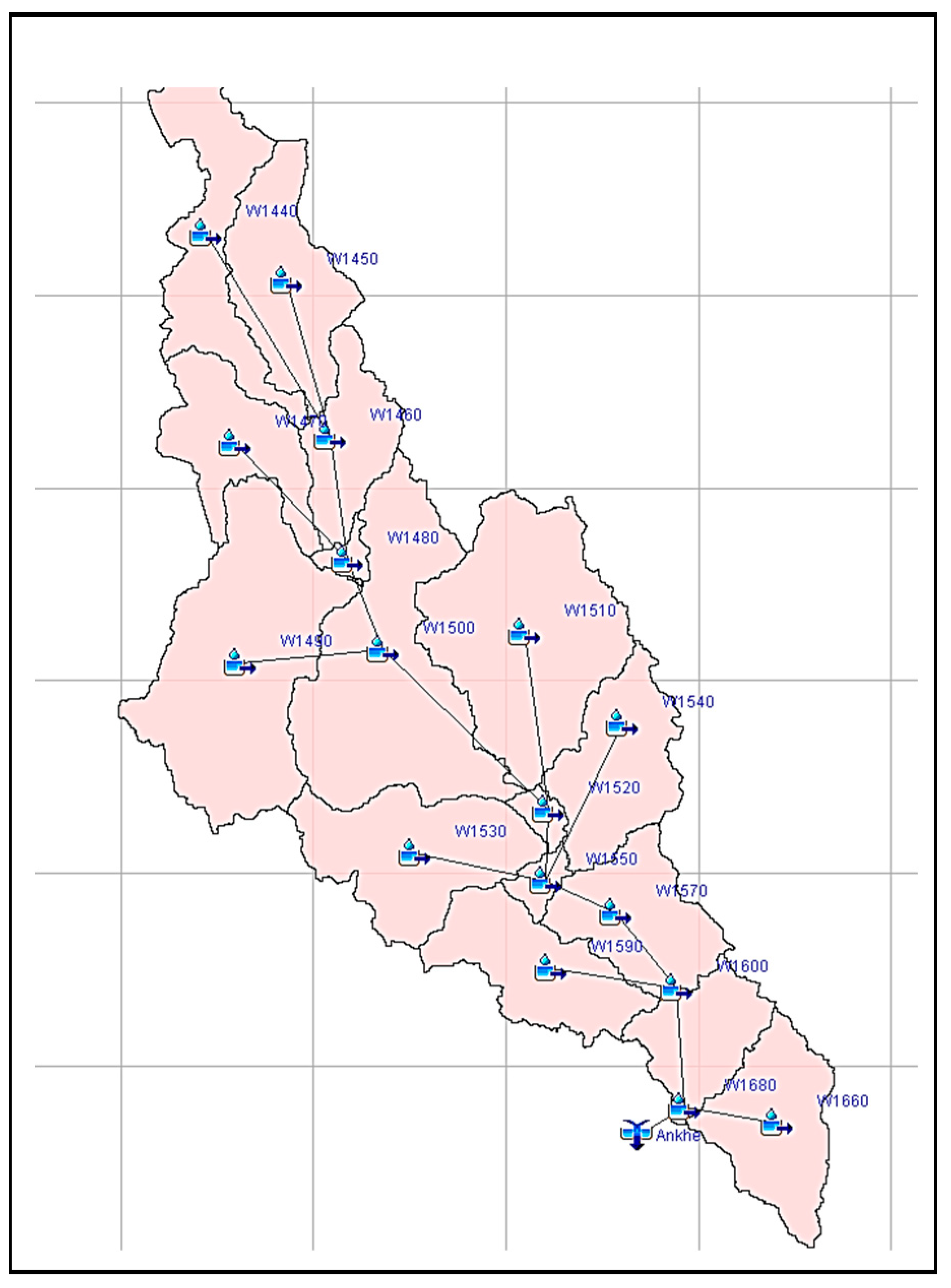
For this study, the catchment was divided into 16 subcatchments as shown in Figure 2 based on DEM with a horizontal resolution of 90 m. Shown in Table 1 are the primary parameters for each subcatchment. As can be seen from that table, each subcatchment requires 10 parameter categories to be estimated. A total of model parameters considered is 16 × 10 = 160 which are from 10 categories. To reduce number of parameter needed to be considered, two coefficients, namely, mean coefficient (K1) and variation coefficient (K2), were introduced for each category. The mean coefficient represents the average value of the 16 parameters over the catchment, while the variation coefficient represents the variation of these values across the catchment.
Sensitivity analyses of HEC-HMS model parameters have been reported (e.g., [37,38,39,40]). From analysis of these studies, it has been found that there are five parameter categories including curve number, representative slope, typical length, roughness, and manning coefficient, that are sensitive and need to be considered during the calibration process.
Further analysis of parameter refining reported in Cu [41] shows application of a variation coefficient (K2) for all the parameter categories results in noise or accumulation of parameter adjusted values. Therefore, selection of one representative variation coefficient for each rainfall-runoff process was preferred. As a result, the variation coefficient was applied to only three parameter categories: Curve Number, Subcatchment Roughness, and Channel Manning. The system, therefore, decreased to eight parameters, namely vector θ. This included K1 for Curve Number (K1—CN); K2 for Curve Number (K2—CN); K1 for Subcatchment Slope (K1—Slope); K1 for Subcatchment Length (K1—length); K1 for Subcatchment Roughness (K1—Catchment Roughness); K2 for Subcatchment Roughness (K2—Catchment Roughness); K1 for Channel Manning (K1—Channel Manning); and K2 for Channel Manning (K2—Channel Manning).
4.4. Uncertainty in Design Flood Flows—FFA Method
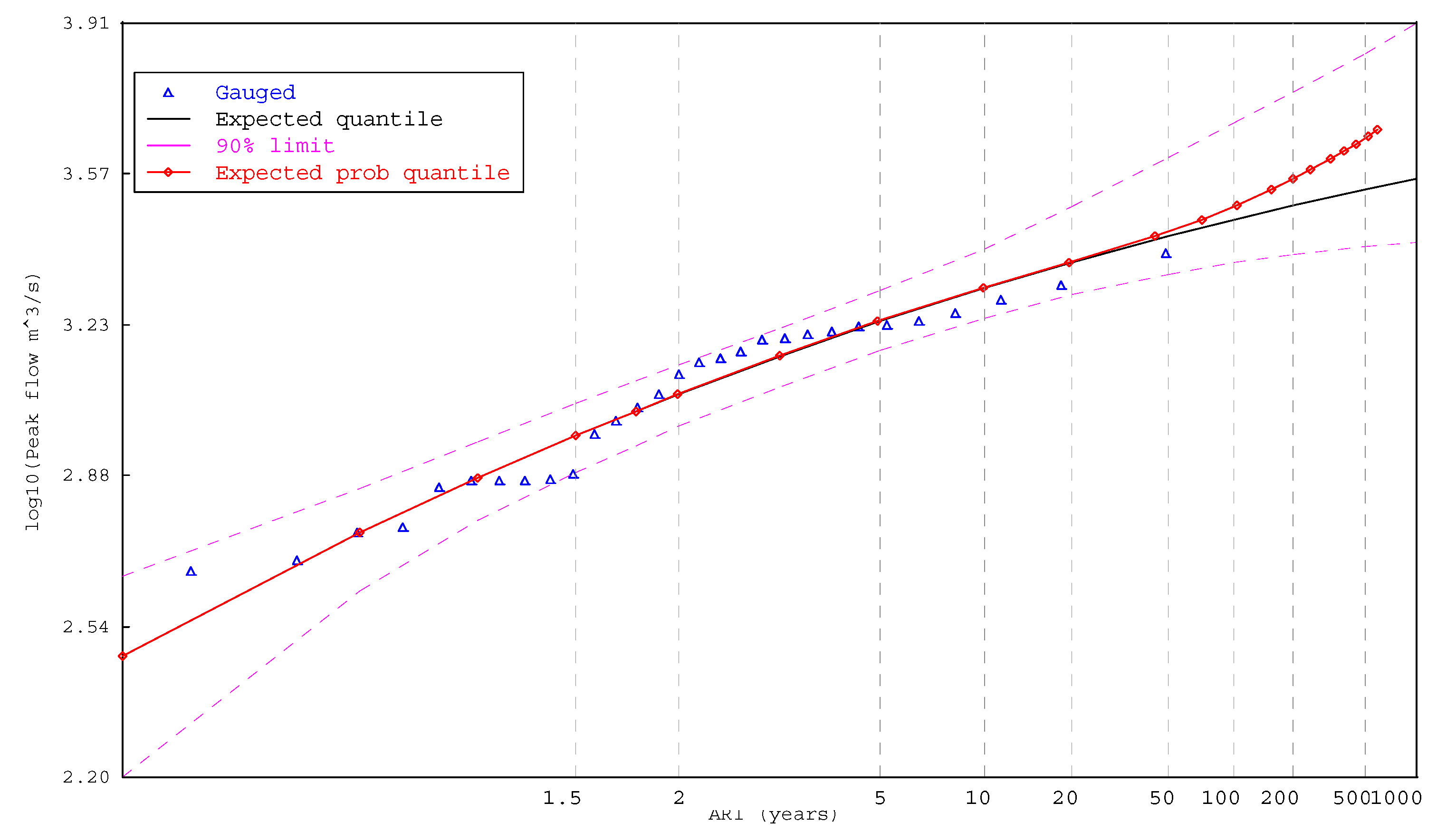
Design flood flows at An Khe station were estimated from the historical data using flood frequency analysis (FFA). Flood quantiles were estimated using FLIKE software [33] with an LP-III distribution and Bayesian parameter estimation. In general, use of the LP-III distribution produced consistent results with, in the majority of cases, the observed data within the confidence limits as shown in Figure 3. Vector , therefore, consists of the location, scale, and shape parameters of LP-III distribution parameters. The most probable value of the location parameter (mean of log flow) is 7.0422, while a standard deviation is 0.09018. In a similar manner, the most probable value of the scale parameter (loge [standard deviation (loge flow)]) is −0.74320 and the standard deviation of scale parameter is 0.15064. Finally, the most probable value of the shape parameter (skewness) is −0.56875 and the standard deviation is 0.45883 (Table 2).
4.5. Likelihood Function
The objective used in the calibration process was vector β estimated by FLIKE as mentioned above.
In the Bayesian method, the likelihood function was normal distribution of location parameter of vector β with most probable values of 7.042 and standard deviation of 0.090 (Table 2).
When applying the GLUE method, the likelihood function used was thresholds of vector β. These thresholds were identified by the values that were one standard deviation away from the mean. Hence, the maximum and minimum of acceptable ranges of β are shown in Table 2.
4.6. Calibration Process
The model was operated at hourly step to predict continuous flow records for the period 1980 to 2011. These generated flow sequences were used to estimate predicted vector βsim. The model parameter sets that resulted in vector βsim met the objective function were selected.
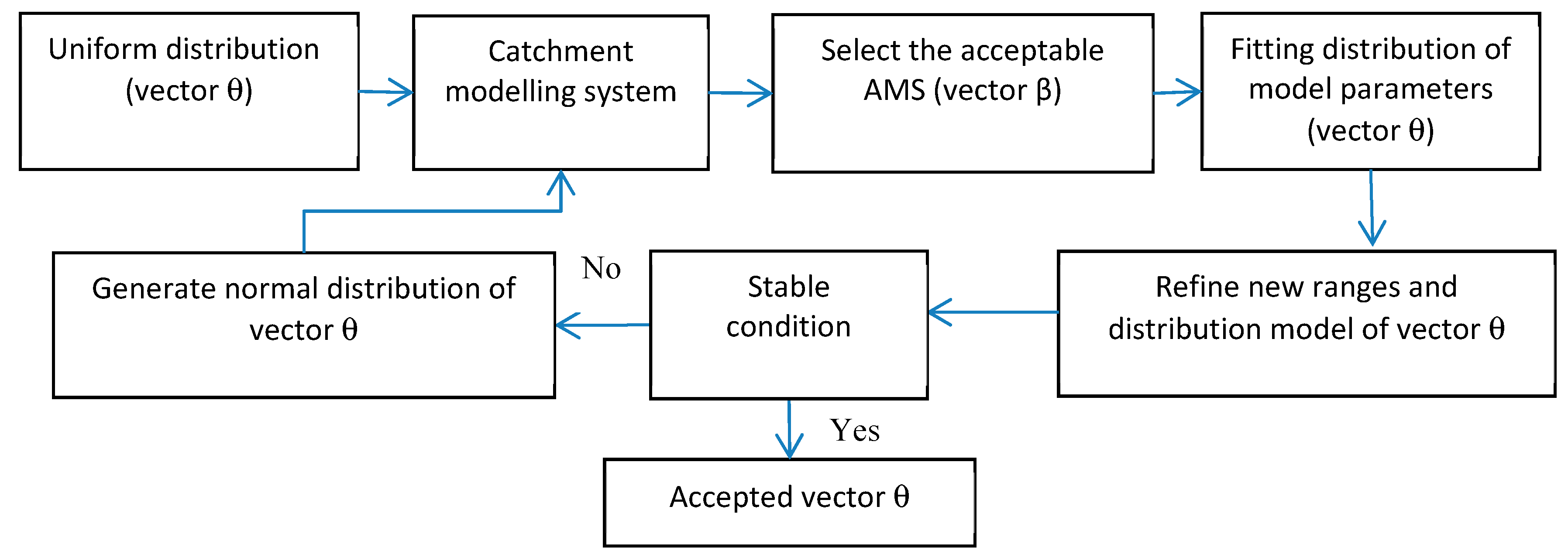
As the catchment modelling system evaluated the uncertainty based on generating a large number of simulations, both manual and computerized techniques have been used for conducting the calibration process. Among the many ways available to assess the uncertainty (e.g., [42,43,44]), the approach adopted assumes the model parameters (vector θ) are random variables. A probability distribution as discussed in the methodology section was done using the monitored procedure as shown in Figure 4.
Step 1—Generation of parameter sets followed a uniform distribution.
As the prior distribution of model parameter values was unknown, a uniform distribution was assumed due to its simplicity. Mersenne-Twister algorithm [45] was used as the random number generator to generate 600 parameter sets within allowable ranges.
Step 2—Application of catchment modelling system (CMS) and selection of acceptable vector θ.
Step 3—Fitting distribution (in Bayesian approach)/or selection of values within the acceptable range (in GLUE) and refining the new ranges of vector θ.
The selected values of vector θ were fitted by a normal distribution. Shapiro-Wilk test [46] was applied to test the normality of the model coefficient distributions. The distributions were assumed to be a new range for generating vector θ in the next step.
Step 4—Generation of new vector θ.
The generation of new vector θ for the next calibration step was undertaken using the new fitted distribution (normal distribution) and the new fitted probability parameters accordingly.
The process of refining the parameter sets was repeated until the distribution of vector θ was stable or 90% of the generated parameter sets produced acceptable AMSs.
5. Results
The parameter uncertainty and model fitness were tested against 2 criteria: (1) Are these parameter set values normally distributed? (2) If yes, is there significant difference between two sets of these data? These criteria were tested using the Shapiro-Wilk test [46] and Welch Two Sample t-test [47].
The Shapiro–Wilk test is a test of normality in frequentist statistics of a data set. The difference between two normal distributed data sets was tested using Welch Two Sample t-test. Both test algorithms use p-value to accept or reject null-hypothesis. If the p-value is less than the chosen alpha level, then the null hypothesis is rejected and there is evidence that the data tested are not from a normally distributed population. Commonly, an alpha level value of 0.05 is accepted [47] which indicates that there are less than five chances out of a hundred that your sample came from a population where that wasn’t true. Hence, the test includes sample size in p value. A p-value of more than 0.05 indicates acceptability in the normality of a distribution and the similarity between two data sets.
5.1. Parameter Uncertainty
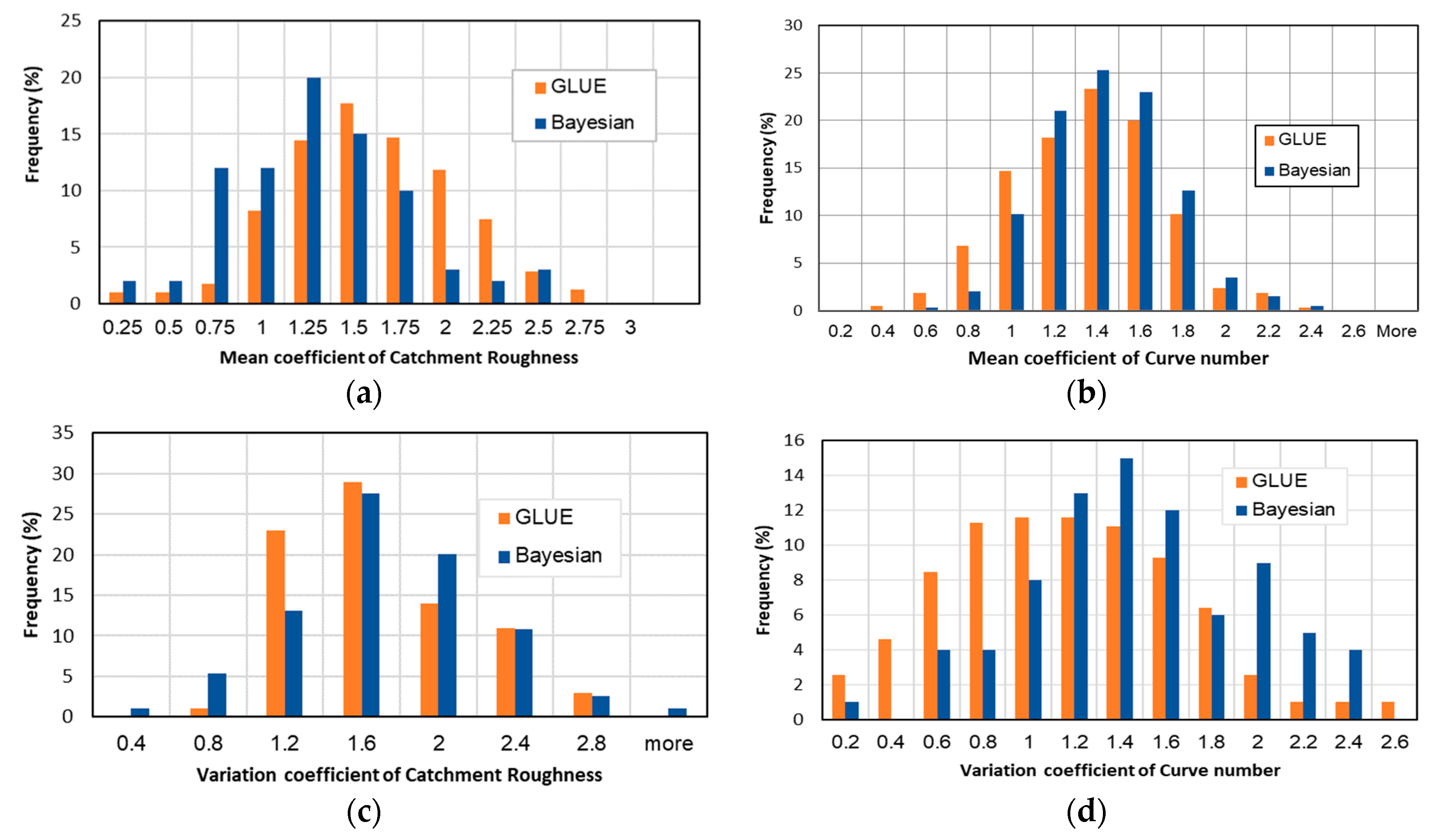
For each method, samples of vector θ which consist of eight posterior coefficient distributions were produced. The Shapiro-Wilk test of normality was used to test normality of the vector θ. All coefficients possess well-defined normal posterior distributions (Figure 5, Table 3). As can be seen from Table 3, the p-values in the normality test for all coefficients were more than 0.05 which is accepted as the standard limit of 95% confidence limits. This indicated that the distributions were considered as being a normal distribution and the sample size of 600 was acceptable. From the distributions, coefficient estimates can be unambiguously inferred as most probable values, while the standard deviation of the distributions indicates the degree of uncertainty of the estimates. With less standard deviation, better coefficients were identified. Flat distributions indicate more coefficient uncertainty.
The similarity of estimates for the GLUE and Bayesian methods were tested by Welch Two Sample t-test. p-values of the testing are reported in Table 3. This indicated that the distribution of most coefficients for GLUE and Bayesian methods were in fact similar. However, the three most sensitive coefficients of the modelling system were statistically different. These coefficients included K1—CN; K2—CN; and K2—Catchment roughness. The differences were indicated by the p value being less than 0.05. The most probable values of K1—CN estimated by the GLUE approach were 1.277, while those values estimated by Bayesian approach were 1.3881. This explained the 8% difference. The difference in K2—CN and K2—catchment roughness was 24% and 35%, respectively.
The posterior distributions obtained by the two methods were somehow similar. This was indicated by a slight difference between standard deviations obtained by the two methods (Table 3). Also, the standard deviations obviously vary across coefficients. Overall the posterior distributions obtained by the Bayesian method were slightly sharper and narrower than those obtained via the GLUE method. This revealed slightly better identified parameters and less uncertainty in parameters in the Bayesian approach.
5.2. Model Goodness of Fit
The goodness of fit was established by two criteria: (1) comparison of fitted vector β (LP-III distribution parameters) against the observed parameters; and (2) comparison of design flood quantiles at 3 average recurrence intervals (ARI): 10, 20 and 50 years ARIs.
Bayesian method:
(1) comparison of fitted vector β: As the fitting distribution method was applied for the Bayesian model, a series of location parameter values obtained from the simulated AMSs was extracted and fitted by a normal distribution. The Shapiro-Wilk test of normality resulted in a p-value of 0.9158 (Table 4) which indicated that the distribution was considered normal. The mean and standard deviations of estimated location parameters were 7.042 and 0.086, respectively (Table 4). The t-test between the observed location parameter and simulated location parameter resulted in similarity, with p-values estimated to be 0.358. Scale and shape parameter values were not from the same populations but they were within the thresholds accordingly.
(2) comparison of design flood quantiles: The simulated AMSs were used to estimate design flow quantiles. All simulated quantiles possessed well-defined normal distributions with p-values of 0.6697, 0.7692, and 0.8581 for 10-year, 20-year, and 50-year ARI, respectively. The most probable values of quantiles are reported in Table 4. The testing similarity of flow quantiles with the observed quantiles resulted in p-values of 0.77, 0.37, and 0.09 for 10-year, 20-year, and 50-year ARI, respectively, which suggested the similarity of estimated design quantiles and observed quantiles.
GLUE method:
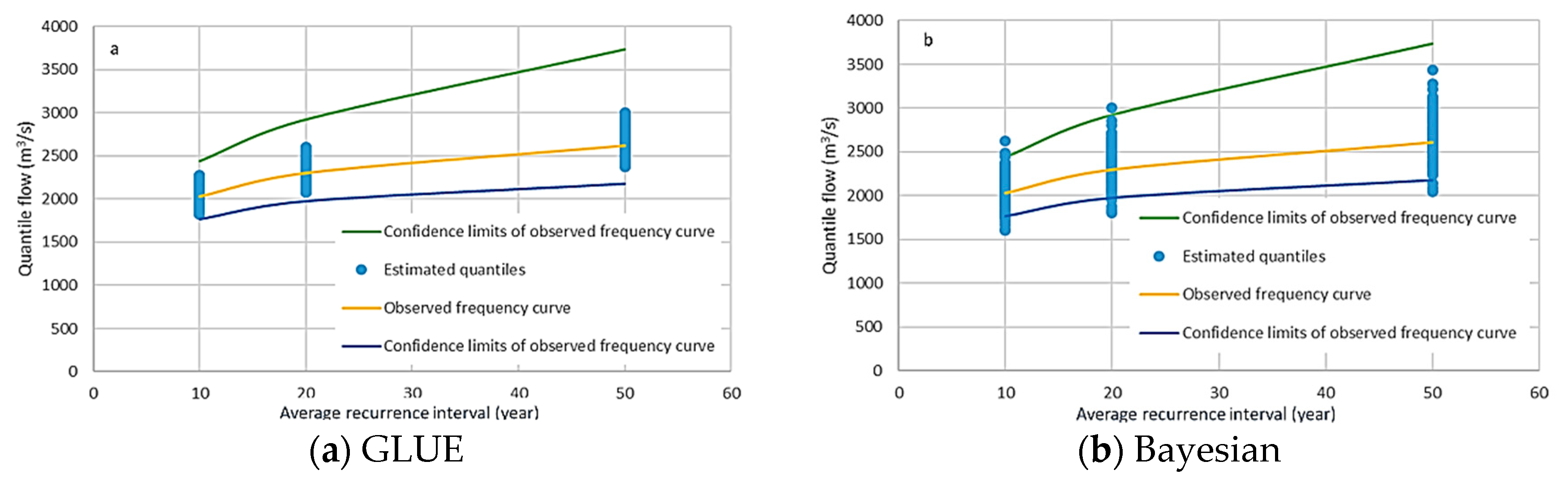
In the GLUE method, the parameter uncertainty results in 90% of simulations which produced AMS parameters (vector β) fitted within the thresholds. The analysis of estimated vector β failed to fit the parameter values with a normal distribution as indicated by p-values of 6.27 × 10⁻⁸. The design flow quantiles of the selected ARI were estimated and shown in Figure 6.
5.3. Uncertainty in Design Flow Quantiles Due to Parameter Uncertainty
The 95% confidence intervals of most probable values of quantiles due to parameter uncertainty were estimated. Table 5 and Figure 6 illustrate the uncertainty of the three quantiles, for example. Compared to the Bayesian method, the flow quantiles estimating the GLUE method were less scattered and located within the confidence limits of the observed frequency curve. However, flow quantiles estimated by the Bayesian approach were normally distributed and statistically were similar to the observed flow quantiles. This was indicated by p-value in t-test equal to 0.09 to 0.77. Meanwhile the flow quantiles resulted in the GLUE method were performed by random scatter. It was subsequently unable to identify the most probable values estimated by the GLUE approach or predict the flows with a given confidence limits. The ranges of quantiles via the GLUE method were estimated (Table 5).
6. Discussion
In this study, a Bayesian approach was applied for parameter estimation with the assumption that the catchment parameters followed a normal distribution. In other words, each parameter can be considered as a distribution of possible values. As the catchment consists of a number of parameters, the study used a joint distribution of these parameters to generate a distribution of model parameter sets that are tested for acceptability. By application of this approach, the study presented a flexible selection approach for model parameters with a statistical representation of each parameter value.
For design flood purposes, the flood flow quantiles were selected as an objective of model calibration. These quantiles can be estimated from the frequency curves. Therefore, three parameters (vector β) of the frequency curves have been selected as a metric for model calibration. The paper introduced two objective functions to treat vector β including a normal distribution of vector β, known as Bayesian approach, and threshold of vector β (1 standard deviation from the mean), namely a GLUE approach.
Both GLUE and Bayesian methods resulted in successfully finding a posterior normal distribution of model parameter values. However, there is a statistical difference in the parameter means estimated from these two approaches and a slight difference between standard deviations of the posterior distributions. The posterior distributions obtained by the Bayesian method were slightly sharper and narrower than those obtained via the GLUE method. This indicated that there were differences in parameter values estimated from the two approaches. The sharper and narrower distributions in Bayesian approach revealed less uncertainty in parameters and hence better identified parameters.
Comparing the quantiles estimated from these approaches shows a greater scatter of the quantile flows for the Bayesian approach than for the GLUE approach. This is due to the assumption of a distribution for vector β that has two tails while the GLUE approach used a cut-off threshold. However, the Bayesian method is successful in fitting a normal distribution of the quantiles flow at three testing probabilities of 10, 20, and 50 year ARIs, and identifies the most probable values.
Both methods can successfully fit the model and identify the model parameter values. Nonetheless, the Bayesian method has an advantage in terms of statistics representation of both objectives and model parameters. Hence this method is more reliable, and better fitted to this catchment.
7. Conclusions
The paper showed that both GLUE and Bayesian methods resulted in successfully simulating the hydrological behavior of the catchment where model parameter sets are accepted as the most probable value and a distribution (normal distribution). The following conclusions are drawn from the study:
Using AMS statistics as the objective function in the calibration process made it possible to identify the likelihood function of the Bayesian method and thresholds for selection of acceptably predicted AMSs in the GLUE method.
The results of calibration revealed there was a statistical difference in several sensitive model parameters estimated by Bayesian and GLUE methods.
Advantage of Bayesian approach compared with GLUE approach in applying the Mersenne-Twister algorithm with an assumption of normal distribution of the parameters as presented in this paper will take into account the impact of low probability parameter values on the generation of parameter values at each calibration step. This indicates that the Bayesian method is more efficient in reproduction of quantile flows.
There are some limitations associated with this method. The method requires a long observation period and rainfall data record for conducting AMS estimation. This case study, Ba River in Vietnam, used a 31-year simulation period, specifically 1980 to 2010. The AMS, therefore, consisted of only 31 records. Even though the study used statistical tests to evaluation model fitness, which allowed the inclusion of sample size in uncertainty of the estimates, and there is no independent validation applied for statistic tests that have been reported before, the small sample size still may result in larger confidence limits of objectives (vector β), which result in higher uncertainty of predicted flows. Therefore, further investigation is needed on how the length of the records impacts on the parameter uncertainty. In addition, as the paper introduced the FFA method in quantile estimation, any uncertainty in model parameters will result in secondary uncertainty of the quantile flows. This, however, is beyond the scope of the paper and will require further study.
Author Contributions
Conceptualisation, P.C.T., J.E.B.; Software, P.C.T.; Investigation, P.C.T., N.H.D., J.E.B.; Writing–Original Draft, P.C.T., N.H.D.; Writing–Review and Editing, J.E.B.; Supervision, J.E.B.
Funding
Support for the first author was provided by a post-thesis scholarship from University of Technology, Sydney (UTS). The support of UTS in this scholarship scheme is gratefully acknowledged.
Acknowledgments
Support for the first author was provided by a post-thesis scholarship from University of Technology, Sydney (UTS). The support of UTS in this scholarship scheme is gratefully acknowledged.
Conflicts of Interest
The authors declare no conflict of interest.
References
- Kuczera, G.; Kavetski, D.; Franks, S.; Thyer, M. Towards a Bayesian total error analysis of conceptual rainfall-runoff models: Characterising model error using storm-dependent parameters. J. Hydrol. 2006, 331, 161–177. [Google Scholar] [CrossRef]
- Xu, C.-Y.; Tunemar, L.; Chen, Y.D.; Singh, V.P. Evaluation of seasonal and spatial variations of lumped water balance model sensitivity to precipitation data errors. J. Hydrol. 2006, 324, 80–93. [Google Scholar] [CrossRef]
- Refsgaard, J.C.; Storm, B. Construction, calibration and validation of hydrological models. In Distributed Hydrological Modelling; Abbott, M.B., Refsgaard, J.C., Eds.; Water Science and Technology Library; Springer: Dordrecht, Germany, 1990; Volume 22, pp. 41–54. [Google Scholar]
- Cameron, D.; Beven, K.; Naden, P. Flood frequency estimation by continuous simulation under climate change (with uncertainty). Hydrol. Earth Syst. Sci. 2000, 4, 393–405. [Google Scholar] [CrossRef] [Green Version]
- Charalambous, J.; Rahman, A.; Carroll, D. Application of Monte Carlo Simulation Technique to Design Flood Estimation: A Case Study for North Johnstone River in Queensland, Australia. Water Resour. Manag. 2013, 27, 4099–4111. [Google Scholar] [CrossRef]
- Frost, A.J.; Thyer, M.A.; Srikanthan, R.; Kuczera, G. A general Bayesian framework for calibrating and evaluating stochastic models of annual multi-site hydrological data. J. Hydrol. 2007, 340, 129–148. [Google Scholar] [CrossRef]
- Aronica, G.T.; Franza, F.; Bates, P.D.; Neal, J.C. Probabilistic evaluation of flood hazard in urban areas using Monte Carlo simulation. Hydrol. Process. 2012, 26, 3962–3972. [Google Scholar] [CrossRef]
- Sikorska, A.E. Interactive comment on Bayesian uncertainty assessment of flood predictions in ungauged urban basins for conceptual rainfall-runoff models. Hydrol. Earth Syst. Sci. Discuss. 2012, 2, C6284–C6310. [Google Scholar]
- Paquet, E.; Garavaglia, F.; Garçon, R.; Gailhard, J. The SCHADEX method: A semi-continuous rainfall–runoff simulation for extreme flood estimation. J. Hydrol. 2013, 495, 23–37. [Google Scholar] [CrossRef]
- Zhou, R.; Li, Y.; Lu, D.; Liu, H.; Zhou, H. An optimization based sampling approach for multiple metrics uncertainty analysis using generalized likelihood uncertainty estimation. J. Hydrol. 2016, 540, 274–286. [Google Scholar] [CrossRef]
- Heidari, A.; Saghafian, B.; Maknoon, R. Assessment of flood forecasting lead time based on generalized likelihood uncertainty estimation approach. Stoch. Environ. Res. Risk Assess. 2006, 20, 363–380. [Google Scholar] [CrossRef]
- Beven, K.; Binley, A. The future of distributed models: Model calibration and uncertainty prediction. Hydrol. Process. 1992, 6, 279–298. [Google Scholar] [CrossRef]
- Beven, K.; Binley, A. GLUE: 20 years on. Hydrol. Process. 2014, 28, 5897–5918. [Google Scholar] [CrossRef]
- Blasone, R.-S.; Vrugt, J.A.; Madsen, H.; Rosbjerg, D.; Robinson, B.A.; Zyvoloski, G.A. Generalized likelihood uncertainty estimation (GLUE) using adaptive Markov Chain Monte Carlo sampling. Adv. Water Resour. 2008, 31, 630–648. [Google Scholar] [CrossRef] [Green Version]
- Bates, P.D.; Horritt, M.S.; Aronica, G.; Beven, K. Bayesian updating of flood inundation likelihoods conditioned on flood extent data. Hydrol. Process. 2004, 18, 3347–3370. [Google Scholar] [CrossRef]
- Xu, W.; Jiang, C.; Yan, L.; Li, L.; Liu, S. An Adaptive Metropolis-Hastings Optimization Algorithm of Bayesian Estimation in Non-Stationary Flood Frequency Analysis. Water Resour. Manag. 2018, 32, 1343–1366. [Google Scholar] [CrossRef]
- Kuczera, G.; Parent, E. Monte Carlo assessment of parameter uncertainty in conceptual catchment models: The Metropolis algorithm. J. Hydrol. 1998, 211, 69–85. [Google Scholar] [CrossRef]
- Gaume, E.; Gaál, L.; Viglione, A.; Szolgay, J.; Kohnová, S.; Blöschl, G. Bayesian MCMC approach to regional flood frequency analyses involving extraordinary flood events at ungauged sites. J. Hydrol. 2010, 394, 101–117. [Google Scholar] [CrossRef]
- Mcmillan, H.; Clark, M. Rainfall-runoff model calibration using informal likelihood measures within a Markov chain Monte Carlo sampling scheme. Water Resour. Res. 2009, 45, W04418. [Google Scholar] [CrossRef]
- Zhao, D.; Chen, J.; Wang, H.; Tong, Q. Application of a Sampling Based on the Combined Objectives of Parameter Identification and Uncertainty Analysis of an Urban Rainfall-Runoff Model. J. Irrig. Drain. Eng. 2013, 139, 66–74. [Google Scholar] [CrossRef]
- Cameron, D.; Beven, K.; Tawn, J.; Naden, P. Flood frequency estimation by continuous simulation (with likelihood based uncertainty estimation). Hydrol. Earth Syst. Sci. 1999, 4, 23–34. [Google Scholar] [CrossRef]
- Shen, Z.Y.; Chen, L.; Chen, T.; Di Baldassarre, G. Analysis of parameter uncertainty in hydrological and sediment modeling using GLUE method: A case study of SWAT model applied to Three Gorges Reservoir Region, China. Hydrol. Earth Syst. Sci. 2012, 16, 121–132. [Google Scholar] [CrossRef]
- Calver, A.; Lamb, R. Flood frequency estimation using continuous rainfall-runoff modelling. Phys. Chem. Earth 1995, 20, 479–483. [Google Scholar] [CrossRef]
- Calver, A.; Stewart, E.; Goodsell, G. Comparative analysis of statistical and catchment modelling approaches to river flood frequency estimation. J. Flood Risk Manag. 2009, 2, 24–31. [Google Scholar] [CrossRef]
- Blazkova, S.; Beven, K. Flood frequency estimation by continuous simulation of subcatchment rainfalls and discharges with the aim of improving dam safety assessment in a large basin in the Czech Republic. J. Hydrol. 2004, 292, 153–172. [Google Scholar] [CrossRef]
- Gioia, A.; Manfreda, S.; Iacobellis, V.; Fiorentino, M. Performance of a theoretical model for the description of water balance and runoff dynamics in Southern Italy. J. Hydrol. Eng. 2014, 19, 1113–1123. [Google Scholar] [CrossRef]
- Stedinger, J.R.; Vogel, R.M.; Lee, S.U.; Batchelder, R. Appraisal of the generalized likelihood uncertainty estimation (GLUE) method. Water Resour. Res. 2008, 44, W00B06. [Google Scholar] [CrossRef]
- Jin, X.; Xu, C.-Y.; Zhang, Q.; Singh, V.P. Parameter and modeling uncertainty simulated by GLUE and a formal Bayesian method for a conceptual hydrological model. J. Hydrol. 2010, 383, 147–155. [Google Scholar] [CrossRef]
- Vrugt, J.A.; Ter Braak, C.J.F.; Gupta, H.V.; Robinson, B.A. Equifinality of formal (DREAM) and informal (GLUE) Bayesian approaches in hydrologic modeling? Stoch. Environ. Res. Risk Assess. 2009, 23, 1011–1026. [Google Scholar] [CrossRef]
- Tang, Y.; Marshall, L.; Sharma, A.; Smith, T. Tools for investigating the prior distribution in Bayesian hydrology. J. Hydrol. 2016, 538, 551–562. [Google Scholar] [CrossRef]
- Smith, T.; Marshall, L.; Sharma, A. Modeling residual hydrologic errors with Bayesian inference. J. Hydrol. 2015, 528, 29–37. [Google Scholar] [CrossRef]
- Dotto, C.B.S.; Mannina, G.; Kleidorfer, M.; Vezzaro, L.; Henrichs, M.; McCarthy, D.T.; Freni, G.; Rauch, W.; Deletic, A. Comparison of different uncertainty techniques in urban stormwater quantity and quality modelling. Water Res. 2012, 46, 2545–2558. [Google Scholar] [CrossRef] [PubMed]
- Kuczera, G.; Franks, S. At-site flood frequency analysis. In Australian Rainfall and Runoff: A Guide to Flood Estimation; Ball, J.E., Babister, M., Nathan, R., Weeks, W., Weinmann, E., Retallick, M., Testoni, I., Eds.; Commonwealth of Australia: Canberra, Australia, 2016; ISBN 978-192529-7072. [Google Scholar]
- Cu, P.T.; Ball, J.E. The influence of the calibration metric on design flood estimation using continuous simulation. Int. J. River Basin Manag. 2016, 15, 9–20. [Google Scholar] [CrossRef]
- Viện khoa học Khí tượng Thủy văn & Môi trường (Kttv&MT). Đánh giá tác động của biến đổi khí hậu lên tài nguyên nước và các biện pháp thích ứng—Lưu vực sông Ba; Trung tâm nghiên cứu thủy văn và môi trường, Viện khoa học Khí Tượng Thủy văn & Môi trường: Hà Nội, Việt Nam, 2010; (Institute of Hydrometeorological and Environment. Assessment of Climate Change Impacts on Water Resources and Adaptation Measures—Ba River Basin; Center of Hydrology and Environment, Institute of Hydro-meteorology & Environment: Hanoi, Vietnam, 2010).
- Ball, J.E.; Cu, T.P. Daily Rainfall Disaggregation for a Monsoon Catchment in Vietnam. In Proceedings of the Hydrology & Water Resources Symposium, Perth, Australia, 24–27 February 2014. [Google Scholar]
- Al-Hamdan, O. Sensitivity Analysis of HEC-HMS Hydrologic Model to the Number of Sub-basins: Case Study. World Environ. Water Resour. Congr. 2009, 2009, 1–9. [Google Scholar]
- Eslamian, S. (Ed.) Handbook of Engineering Hydrology: Fundamentals and Applications; Francis and Taylor, CRC Group: Boca Raton, FL, USA, 2014. [Google Scholar] [CrossRef]
- Kousari, M.R.; Malekinezhad, H.; Ahani, H.; Zarch, M.A. Sensitivity Analysis and Impact Quantification of the Main Factors Affecting Peak Discharge in the SCS Curve Number Method: An Analysis of Iranian Watersheds. Quat. Int. 2010, 226, 66–74. [Google Scholar] [CrossRef]
- US Army Corps of Engineers. Hydrologic Modeling System HEC-HMS; Technical Reference Manual; Hydrologic Engineering Center: Davis, CA, USA, 2000.
- Cu, P.; Ball, J.E. Parameter estimation for a large catchment. Australas. J. Water Resour. 2017, 21, 20–33. [Google Scholar] [CrossRef]
- Franz, K.J.; Hogue, T.S. Evaluating uncertainty estimates in hydrologic models: Borrowing measures from the forecast verification community. Hydrol. Earth Syst. Sci. Discuss. 2011, 8, 3085–3131. [Google Scholar] [CrossRef]
- Del Giudice, D.; Honti, M.; Scheidegger, A.; Albert, C.; Reichert, P.; Rieckermann, J. Improving uncertainty estimation in urban hydrological modeling by statistically describing bias. Hydrol. Earth Syst. Sci. 2013, 17, 4209–4225. [Google Scholar] [CrossRef]
- Dogulu, N.; López, L.P.; Solomatine, D.P.; Weerts, A.H.; Shrestha, D.L. Estimation of predictive hydrologic uncertainty using the quantile regression and UNEEC methods and their comparison on contrasting catchments. Hydrol. Earth Syst. Sci. 2015, 19, 3181–3201. [Google Scholar] [CrossRef] [Green Version]
- Matsumoto, M.; Nishimura, T. Mersenne twister: A 623-dimensionally equidistributed uniform pseudo-random number generator. ACM Trans. Model. Comput. Simul. 1998, 8, 3–30. [Google Scholar] [CrossRef]
- Patrick, R. Algorithm AS 181: The W test for Normality. Appl. Stat. 1982, 31, 176–180. [Google Scholar] [CrossRef]
- Welch, B.L. On the Comparison of Several Mean Values: An Alternative Approach. Biometrika 1951, 38, 330–336. [Google Scholar] [CrossRef]
Figure 1.
Distribution of meteorological stations across Ba River catchment.

Figure 2.
Catchment delineation and stream network.

Figure 3.
Flood frequency curve at An Khe gauge [34].
Figure 3.
Flood frequency curve at An Khe gauge [34].

Figure 4.
Scheme for the calibration process.

Figure 5.
Histogram of mean and variation coefficients estimated by Bayesian and Generalized Likelihood Uncertainty Estimation (GLUE) method. (a) K1-catchment roughness, (b) K1—CN, (c) K2—Catchment Roughness and (d) K2—CN.
Figure 5.
Histogram of mean and variation coefficients estimated by Bayesian and Generalized Likelihood Uncertainty Estimation (GLUE) method. (a) K1-catchment roughness, (b) K1—CN, (c) K2—Catchment Roughness and (d) K2—CN.

Figure 6.
Uncertainty of design flood quantiles estimated using the GLUE (a) and Bayesian (b) methods.
Figure 6.
Uncertainty of design flood quantiles estimated using the GLUE (a) and Bayesian (b) methods.


Table 1.
Model parameter categories and their available ranges [40].
Table 1.
Model parameter categories and their available ranges [40].
| Models | Parameter Categories | Range |
|---|---|---|
| Loss models | Curve Number | 20–90 |
| Kinematic wave (Overland flow planes) | Typical length | |
| Representative slope | 0.0001–1 | |
| Overland-flow roughness coefficient | 0.35–0.8 | |
| Area represented by plane | ||
| Muskingum-Cunge routing (The main channel) | Main channel length | |
| Description of main channel shape | Rectangular | |
| Channel slope | 0.0001–1 | |
| Channel width | ||
| Representative Manning’s Roughness coefficient | 0.035–0.08 |
Table 2.
Parameter values of LP-III distribution (vector β) and ranges of acceptable LP-III parameters at An Khe gauge.
Table 2.
Parameter values of LP-III distribution (vector β) and ranges of acceptable LP-III parameters at An Khe gauge.
| N | Parameters | Most Probable Value (α) | Standard Deviation (σ) | Maximum | Minimum |
|---|---|---|---|---|---|
| 1 | Mean (loge flow) | 7.042 | 0.090 | 7.132 | 6.952 |
| 2 | Loge (Std dev (loge flow)) | −0.743 | 0.151 | −0.593 | −0.894 |
| 3 | Skew (loge flow) | −0.569 | 0.459 | −0.110 | −1.028 |
Table 3.
Accepted model coefficients.
| Parameters | GLUE Approach | Bayesian Approach | t-Test | ||||
|---|---|---|---|---|---|---|---|
| Mean | STD | p-Value in Normality Test | Mean | STD | p-Value in Normality Test | p-Value in Similarity Test | |
| K1—CN | 1.278 | 0.314 | 0.111 | 1.388 | 0.308 | 0.691 | 0.0051 |
| K2—CN | 1.038 | 0.474 | 0.811 | 1.369 | 0.475 | 0.409 | 1.422 × 10⁻⁷ |
| K1—Slope | 0.664 | 0.125 | 0.376 | 0.647 | 0.189 | 0.911 | 0.462 |
| K1—Length | 1.812 | 0.379 | 0.994 | 1.785 | 0.377 | 0.440 | 0.567 |
| K1—Catchment Roughness | 1.495 | 0.461 | 0.045 | 1.427 | 0.474 | 0.181 | 0.252 |
| K2—Catchment Roughness | 1.514 | 0.506 | 0.241 | 1.115 | 0.155 | 0.649 | 2.2 × 10⁻¹⁶ |
| K1—Channel Manning | 1.345 | 0.404 | 0.550 | 1.431 | 0.381 | 0.226 | 0.075 |
| K2—Channel Manning | 1.435 | 0.552 | 0.224 | 1.539 | 0.506 | 0.086 | 0.109 |
Table 4.
Most probable values and p-values of t-test design quantiles using the Bayesian method.
| Parameters | Most Probable Values | Standard Deviation | p-Value in Normality Test | Observed Most Probable Values | p-Value in Similarity Test |
|---|---|---|---|---|---|
| Location parameter LP-III distribution | 7.042 | 0.086 | 0.916 | 7.051 | 0.358 |
| Scale parameter LP-III distribution | −0.762 | 0.031 | 0.174 | −0.743 | 1.114 × 10⁻⁶ |
| Shape parameter LP-III distribution | −0.4588 (mean) | −0.409/0.550 (range) | 0.0005 | −0.569 | |
| Q-10 (m3/s) | 2036 | 206.8 | 0.670 | 2029 | 0.774 |
| Q-20 (m3/s) | 2323 | 241.2 | 0.769 | 2299 | 0.379 |
| Q-50 (m3/s) | 2668 | 282.0 | 0.858 | 2614 | 0.092 |
Table 5.
Most probable values and confidence limits of flood flows (observed flows versus estimates).
Table 5.
Most probable values and confidence limits of flood flows (observed flows versus estimates).
| ARI | Observed Quantiles (m3/s) | Quantiles Estimated by the Bayesian Approach (m3/s) | Quantiles Estimated by the GLUE Approach (m3/s) | ||||||
|---|---|---|---|---|---|---|---|---|---|
| Most Probable Values | Lower Confidence Limit | Upper Confidence Limit | Most Probable Value | Lower Confidence Limit (95%) | Upper Confidence Limit (95%) | Mean | Lower Threshold | Upper Threshold | |
| 10 | 2029 | 1768 | 2437 | 2035 | 1623 | 2447 | 2043 | 1827 | 2273 |
| 20 | 2299 | 1978 | 2920 | 2322 | 1840 | 2804 | 2333 | 2075 | 2607 |
| 50 | 2614 | 2182 | 3732 | 2667 | 2105 | 3229 | 2682 | 2370 | 3007 |
© 2018 by the authors. Licensee MDPI, Basel, Switzerland. This article is an open access article distributed under the terms and conditions of the Creative Commons Attribution (CC BY) license (http://creativecommons.org/licenses/by/4.0/).
Share and Cite
MDPI and ACS Style
Cu Thi, P.; Ball, J.E.; Dao, N.H. Uncertainty Estimation Using the Glue and Bayesian Approaches in Flood Estimation: A case Study—Ba River, Vietnam. Water 2018, 10, 1641. https://doi.org/10.3390/w10111641
AMA Style
Cu Thi P, Ball JE, Dao NH. Uncertainty Estimation Using the Glue and Bayesian Approaches in Flood Estimation: A case Study—Ba River, Vietnam. Water. 2018; 10(11):1641. https://doi.org/10.3390/w10111641
Chicago/Turabian StyleCu Thi, Phuong, James E Ball, and Ngoc Hung Dao. 2018. "Uncertainty Estimation Using the Glue and Bayesian Approaches in Flood Estimation: A case Study—Ba River, Vietnam" Water 10, no. 11: 1641. https://doi.org/10.3390/w10111641
Note that from the first issue of 2016, this journal uses article numbers instead of page numbers. See further details here.