Theoretical Model of Suspended Sediment Concentration in a Flow with Submerged Vegetation

Abstract

Vegetation in natural river interacts with river flow and sediment transport. This paper proposes a two-layer theoretical model based on diffusion theory for predicting the vertical distribution of suspended sediment concentration in a flow with submerged vegetation. The suspended sediment concentration distribution formula is derived based on the sediment and momentum diffusion coefficients through the inverse of turbulent Schmidt number ($S{c}_t$) or the parameter $\eta$ which is defined by the ratio of sediment diffusion coefficient to momentum diffusion coefficient. The predicted profile of suspended sediment concentration moderately agrees with the experimental data. Sensitivity analyses are performed to elucidate how the vertical distribution profile responds to different canopy densities, hydraulic conditions and turbulent Schmidt number. Dense vegetation renders the vertical distribution profile uneven and captures sediment particles into the vegetation layer. For a given canopy density, the vertical distribution profile is affected by the Rouse number, which determines the uniformity of the sediment on the vertical line. A high Rouse number corresponds to an uneven vertical distribution profile.

1. Introduction

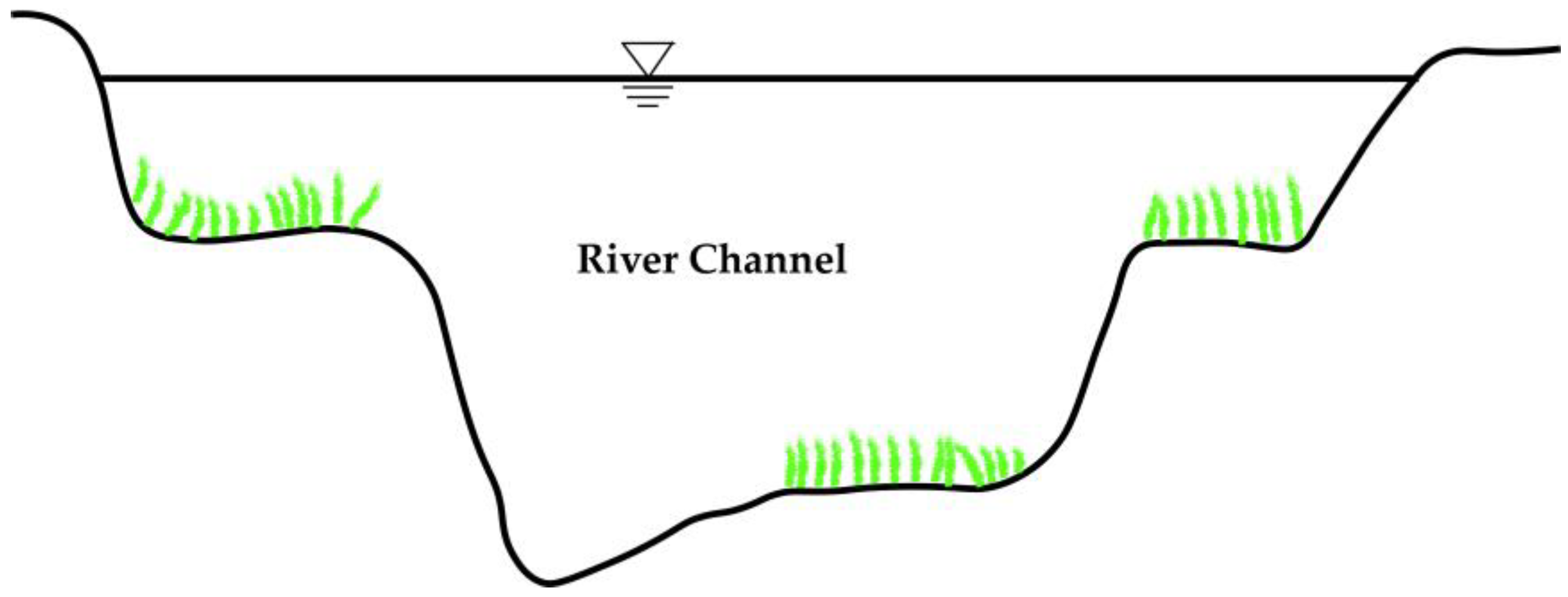
Vegetation is an important part of the river ecosystem. It can exist in the middle channel, grow on the river bed, and populate both terraces and floodplains (Figure 1). Vegetation provides a habitat for aquatic life and greatly influences the hydraulic conditions and morphology in a river ecosystem. For example, canopies in river channels alter the structure of the turbulent flow and the velocity profile. Meanwhile, the changing velocity profile affects the characteristics of sediment transport. The sediment transport characteristics in canopy flow should be identified for the efficient management of floods and the river ecosystem.

The vertical distribution of suspended sediment concentration is a key point to characterize sediment transport. Open channels flows are highly turbulent. Sediment particles are suspended resulting from the combination of the turbulent diffusion of water flow and the action of particle gravity. This basic concept underlies the theory of particle diffusion.

Diffusion theory is widely used in the study of the distribution of suspended particle concentration along the vertical line. In essence, it reflects the continuous equation or mass conservation equation that the suspended particles should satisfy when they are in equilibrium in the water flow. This equation can be expressed by the Schmidt equation [1] as

$${\epsilon }_z\frac{d{S}_v}{dz}+\omega S_v=0$$

(1)

where $S_v$ is the mean concentration and $\omega$ is the settling velocity of sediment particles in still water. The settling velocity is calculated by using the median particle size ($d_{50}$) for non-uniform sediment. In the environment of alluvial rivers with floodplain and low gradient of thalweg, grain sizes of the suspended sediment and bed composition are usually in narrow ranges. Calculation with the median particle size ($d_{50}$) can approximately reflect the movement of particles of all grain sizes. ${\epsilon }_z$ is the vertical diffusion coefficient of suspended particles. If ${\epsilon }_z$ is determined, then we can obtain the suspended sediment concentration by integrating Equation (1). In fact, the diffusion coefficient varies along the water depth. Furthermore, the turbulent diffusion coefficient of suspended sediment ${\epsilon }_z$, which has great influence on the vertical distribution profile of suspended sediment, is somewhat different from the turbulent momentum diffusion coefficient ${\epsilon }_m$ [2]. The turbulent diffusion coefficients are generally predicted in terms of the turbulent Schmidt number ($S{c}_t$) or the parameter $\eta$ which is defined by the ratio of sediment diffusion coefficient to momentum diffusion coefficient [3]. The momentum exchange coefficient ${\epsilon }_m$ can be described by the gradient of velocity ($du/dz$) and the shear stress ($\tau$). Hence, the relationship of the sediment diffusion coefficient and the momentum diffusion coefficient is closely described as

$${\epsilon }_z=\frac{1}{S{c}_t}\cdot {\epsilon }_m=\eta \cdot {\epsilon }_m=\eta \cdot \frac{\tau }{\rho \frac{du}{dz}}$$

(2)

where $\rho$ is the water density.

Suitable available formulas of $\eta$ have been proposed by previous researchers [2,3,4,5,6]. A widely cited expression of $\eta$ is chosen from Tsujimoto and the expression is given by [2]:

$$\eta =1+1.56{\left(\frac{\omega }{u_{\ast }}\right)}^2$$

(3)

where $u_{\ast }$ is the friction velocity. Pal and Goshal [3] investigated the effect of particle concentration on sediment and momentum diffusion coefficients in open-channel sediment-laden turbulent flow for dilute and non-dilute states. They found that with increasing particle concentration, the sediment diffusion coefficient decreases more in comparison with the momentum diffusion coefficient for both dilute and non-dilute sediment-laden flows.

According to Equation (2), the key point to determine the momentum exchange coefficient is the gradient of velocity decided by the vertical velocity distribution. Rouse et al. proposed a model to describe the vertical distribution of suspended sediment concentration in an open-channel flow without vegetation under which condition the longitudinal velocity is logarithmic [7]. The Rouse formula can be expressed as

$$\frac{S_v}{S_{vb}}={\left(\frac{H-z}{z}\frac{b}{H-b}\right)}^{\psi }$$

(4)

where $S_{vb}$ is the mean concentration at $z=b$ and $H$ is the flow depth. $\psi =\omega /\left(\eta \kappa u_{\ast }\right)$ is the suspension index or Rouse number and $\kappa$ is the von Kármán constant.

Yang et al. developed a simple relationship based on the two-layer approach for suspended sediment concentration in a depth-limited flow with submerged canopy [8]. In their study, the longitudinal velocity is assumed to be uniform in the canopy layer and logarithmic in the free water layer. However, a break point exists at the top of the canopy, and the diffusion coefficient in the canopy layer is calculated imprecisely, which undermines the applicability of the model to describe the suspended sediment distribution of submerged canopy flow. Thus, an accurate longitudinal velocity profile is important to establish a model of suspended sediment distribution.

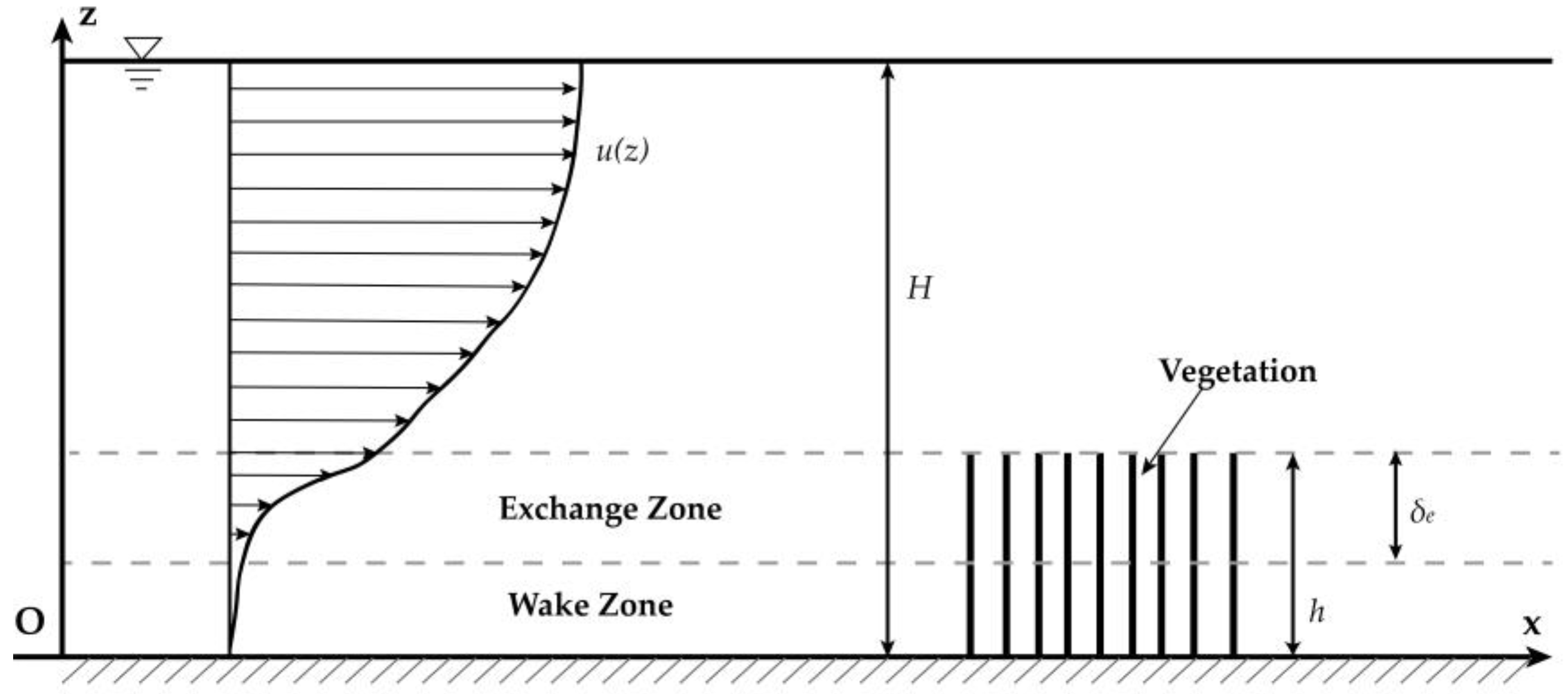
Klopstra et al. proposed analytical expressions for velocity distribution [9]. The velocity profile in the canopy layer is obtained based on the Boussinesq concept, whereas the logarithmic for the free water layer is derived from Prandtl’s mixing length theory. The two-layer approach divides the flow depth into the upper layer and the vegetation layer [8]. In the vegetation layer, the velocity is uniform. Huai et al. proposed a three-layer approach by further dividing the canopy layer into inner and outer layers [10]. Nepf et al. reported that the vertical turbulent structure within a canopy is dominated by the vegetation morphology, which is characterized by the canopy height ($h$) and the plant frontal area per unit canopy volume ($a$) [11]. De Serio et al. analyzed the experimental results which highlighted the importance of the density of the vegetation as a key parameter in the advective processes [12]. The vertical turbulent transport of momentum is driven by the canopy-scale vortices. The region of the canopy affected by these vortices is termed the exchange zone, in which the exponential velocity profile is observed [13]. The length of the exchange zone extends from the top of the vegetation over a distance called the penetration length (Figure 2) is described by the following equation:

$${\delta }_e=\frac{0.23\pm 0.06}{C_{D}a}$$

(5)

where $C_D$ is the canopy drag coefficient defined using a quadratic drag [14,15]. Below the exchange zone, a relatively quiescent area is called the wake zone where the velocity is uniform. Above the submerged canopy, the velocity profile is logarithmic [16].

The study aims to develop a new relationship for suspended sediment transport in a flow with submerged canopy, which is based on a new longitudinal velocity distribution model and the turbulent Schmidt number. The longitudinal velocity profiles, which are logarithmic in the free water layer and exponential in the canopy layer, are adopted and tested, respectively. In this framework, relationships for the vertical distribution of suspended sediment concentration are proposed. Then, the proposed formulas are verified by comparing with the experimental data. Finally, the proposed formulas are used to study the effect of canopy density, hydraulic condition and the turbulent Schmidt number on the vertical distribution of suspended sediment concentration.

2. Methods

2.1. Flow Model

The velocity distribution model adopted in this study is widely cited but relatively simple in structure. It provides great convenience for integral calculation to derive the vertical distribution model of suspended sediment concentration. The flow model is described below.

For a flow with submerged canopy, the vertical distribution of mean velocity from the river bed to the water surface highly depends on the relative importance of the river bed drag and the vegetation drag. If the bed drag plays a dominant role in the flow compared with the canopy drag, then the velocity distribution follows a turbulent boundary-layer profile, whereas the canopy is considered into the bed roughness (sparse canopy). By contrast, if the canopy drag plays the more dominant part compared with the bed drag, the discontinuity in drag that occurs at the top of the canopy ($z=h$) generates a region of a shear resembling a free shear layer with an inflection point near the top of the vegetation (dense canopy) [13]. A pronounced inflection point is expected to appear at the top of the vegetation for $C_{D}ah>0.1$ [13].

To describe the flow velocity $u\left(z\right)$ with submerged canopies, early research reported that $u\left(z\right)$ is a function of only $u_{\ast }$, $a$, $h$ and $C_D$. Kaimal and Finnigan hypothesized that the vertical distribution of mean velocity for a sufficiently far above a submerged canopy ($z>h$) is logarithmic:

$$u\left(z\right)=\frac{u_{\ast }}{\kappa }\ln \left(\frac{z-z_m}{z_0}\right)$$

(6)

where $z_m$ is the displacement height and $z_0$ is the roughness height. The two parameters both depend on the vegetation density. In the previous study [17], the friction velocity in a canopy flow is calculated according to the following formula:

$$u_{\ast }=\sqrt{gS\left(H-h\right)}$$

(7)

were $S=\partial H/\partial x+\sin \theta$ [17] and $\theta$ is the bed slope angle. Jarvela pointed out $h$ is the averaged deflected height of the canopy for flexible vegetation [18]. However, when the relative depth of submergence is small, replacing $h$ with $z_m$ will have more accurate results [19].

The displacement height ($z_m$) is similar with the penetration length scale (${\delta }_e$). It represents the centroid of momentum penetration into the vegetation layer [20]. This similarity suggests the physically intuitive scaling:

$$\frac{z_m}{h}\approx 1-\frac{1}{2}\frac{{\delta }_e}{h}=1-\frac{0.1}{C_{D}ah}$$

(8)

Which has been confirmed for $ah\approx$ 0.2 to 3 [21]. $z_m$ will be zero at $C_{D}ah=0.1$. When $z_m$ approaches zero, no inflection point can be found in the velocity profile. The great sparsity of the canopy exerts a considerable influence on the velocity profile. The traditional logarithmic velocity profile fits the sparse canopy condition well. For $C_{D}ah>1$, the displacement height is approximately equivalent to the canopy height. It denotes that the whole canopy is cut off from the overflow [13].

The roughness height ($z_0$) is heavily affected by the canopy density. The relationship between $z_0$ and $ah$ differs significantly above and below the threshold of $ah=0.1$ [22]. For sparse vegetation, $z_0$ is proportional to the drag generated by the full canopy because the flow penetrates the whole canopy, i.e., $z_0/h\sim C_{D}ah$. On the contrary, the roughness height decreases with the increasing $ah$ for dense canopies. Luhar et al. suggested that for $ah>0.1$, $z_0=\left(0.04\pm 0.02\right)a^{-1}$ [21].

The velocity distribution model adopted in this paper divided the canopy layer into exchange zone and wake zone. And in the wake zone, the longitudinal velocity is uniform while the velocity profile in the exchange zone follows an exponential decay. However, in this paper, the velocity distribution in the wake zone is assumed to be same as the velocity profile in the exchange profile. It is because the gradient of velocity is important for calculating the momentum diffusion coefficient.

Therefore, according to Harman et al. [23] and Nepf [13], the velocity profile below the canopy height follows an exponential decay:

$$u\left(z\right)=u_1+\left(u_h-u_1\right)e^{\frac{\beta \left(z-h\right)}{l}}$$

(9)

where $u_h$ is the velocity at the canopy height ($z=h$) and $u_1=\sqrt{2gS/\left(C_{D}a\right)}$ is the averaged velocity in the wake zone ($z<h-{\delta }_e$). $u_h$ can be calculated by Equation (6). The velocity-decay length-scale ($l/\beta$ in 10) can be determined using a mixing length ($l$) characterization of eddy viscosity, which leads to $\beta =u_{\ast }/u_h$ and $l=2{\beta }^3/C_{D}a$.

2.2. Reynolds Stress Distribution

Under the uniform, steady, and sufficiently developed turbulent open channel flow with submerged canopy, the flow regime can be divided into two layers, the canopy layer ($z<h$) and the free water layer ($z>h$).

Below the canopy height ($z=h$), Shimizu et al. proposed that the Reynolds stress distribution conforms to an exponential profile for rigid canopy [24]. After analyzing a large amount of Reynolds stress data, Dijkstra and Uittenbogaard found that the vertical distribution profiles for both rigid and flexible vegetation are similar, in that the Reynolds stress conforms to an exponential profile and the maximum value is near the top of the canopy [25]. In consideration of this study, the vertical distribution of the Reynolds stress can be described as

$$\tau =-\rho \overline{u^{\prime }{w}^{\prime }}=-\rho {\overline{u^{\prime }{w}^{\prime }}|}_{z=h}{e}^{\alpha \left(z-h\right)}$$

(10)

where $\alpha$ is a constant that can be determined later. $u^{\prime }$ and $w^{\prime }$ are the temporal fluctuations from the means of the longitudinal and vertical velocities, respectively. According to the momentum balance of the flow above the canopy, the interfacial shear stress between canopies can be described as [8]

$$-\rho {\overline{u^{\prime }{w}^{\prime }}|}_{z=h}=\rho gS\left(H-h\right)=\rho u_{\ast }^2$$

(11)

The constant $\alpha$ is related to the flow conditions and the characteristic of the canopy. On the basis of studies with both model and experimental data, a simple estimate for the constant has been obtained by [26]:

$$\alpha =\sqrt{\frac{C_{D}a}{0.03\left(H-h\right)}}$$

(12)

For the free water layer ($z>h$), the eddy viscosity model of Boussinesq was employed to describe the Reynolds shear stress as

$$\tau =\rho {\upsilon }_t\frac{du}{dz}=\rho gS\left(H-z\right)$$

(13)

where ${\upsilon }_t$ is the eddy viscosity.

2.3. Suspended Sediment Concentration Model

Basing from diffusion theory, we assumed that ${\epsilon }_z$ is equivalent to ${\epsilon }_m$. For a uniform, steady, and fully developed turbulent open channel flow with submerged vegetation, the diffusion coefficient ${\epsilon }_z$ can be estimated by combining Equations (6), (9), (10) and (13):

$${\epsilon }_z=\eta \cdot {\epsilon }_m=\eta \cdot \frac{\tau }{\rho \frac{du\left(z\right)}{dz}}=\eta \frac{\kappa gS}{u_{\ast }}\left(H-z\right)\left(z-z_m\right)(z>h)$$

(14)

$${\epsilon }_z=\eta \cdot {\epsilon }_m=\eta \cdot \frac{\tau }{\rho \frac{du\left(z\right)}{dz}}=\eta \frac{gS\left(H-h\right)l}{\beta \left(u_h-u_1\right)}{e}^{\left(\alpha -\frac{\beta }{l}\right)\left(z-h\right)}(z<h)$$

(15)

By integrating Equation (1) using Equations (14) and (15), the vertical distribution of suspended sediment concentration is a submerged canopy flow can be described as

$$\ln \left(\frac{S_v\left(z\right)}{S_v\left(h\right)}\right)=-\frac{\omega }{\eta gS}\frac{u_{\ast }}{\kappa }\frac{1}{H-z_m}\ln \left(\frac{z-z_m}{H-z}\frac{H-h}{h-z_m}\right)(z>h)$$

(16)

$$\ln \left(\frac{S_v\left(h\right)}{S_v\left(z\right)}\right)=-\frac{\omega }{\eta gS}\frac{\beta }{\beta -\alpha l}\frac{u_h-u_1}{H-h}\left[1-e^{\left(\frac{\beta }{l}-\alpha \right)\left(z-h\right)}\right](z<h)$$

(17)

Obviously, the vertical distribution profile is divided into two parts along the flow depth at the top of the canopy. Notably, the sediment particles near the river bed within a certain range do not belong to suspended load. Therefore, the minimum value of $z$ is normally taken as the height equal to 5% of the flow depth ($H$) [8].

As mentioned before, $z_m$ approaches zero when $C_{D}ah\le 0.1$. Thus, the sparse canopy exerts less influence on the velocity profile compared with the flow without vegetation. Actually, for the sparse canopy, Equation (16) can be reduced to the form of the Rouse formula along the full flow depth.

3. Results and Discussion

3.1. Verification of Flow Model

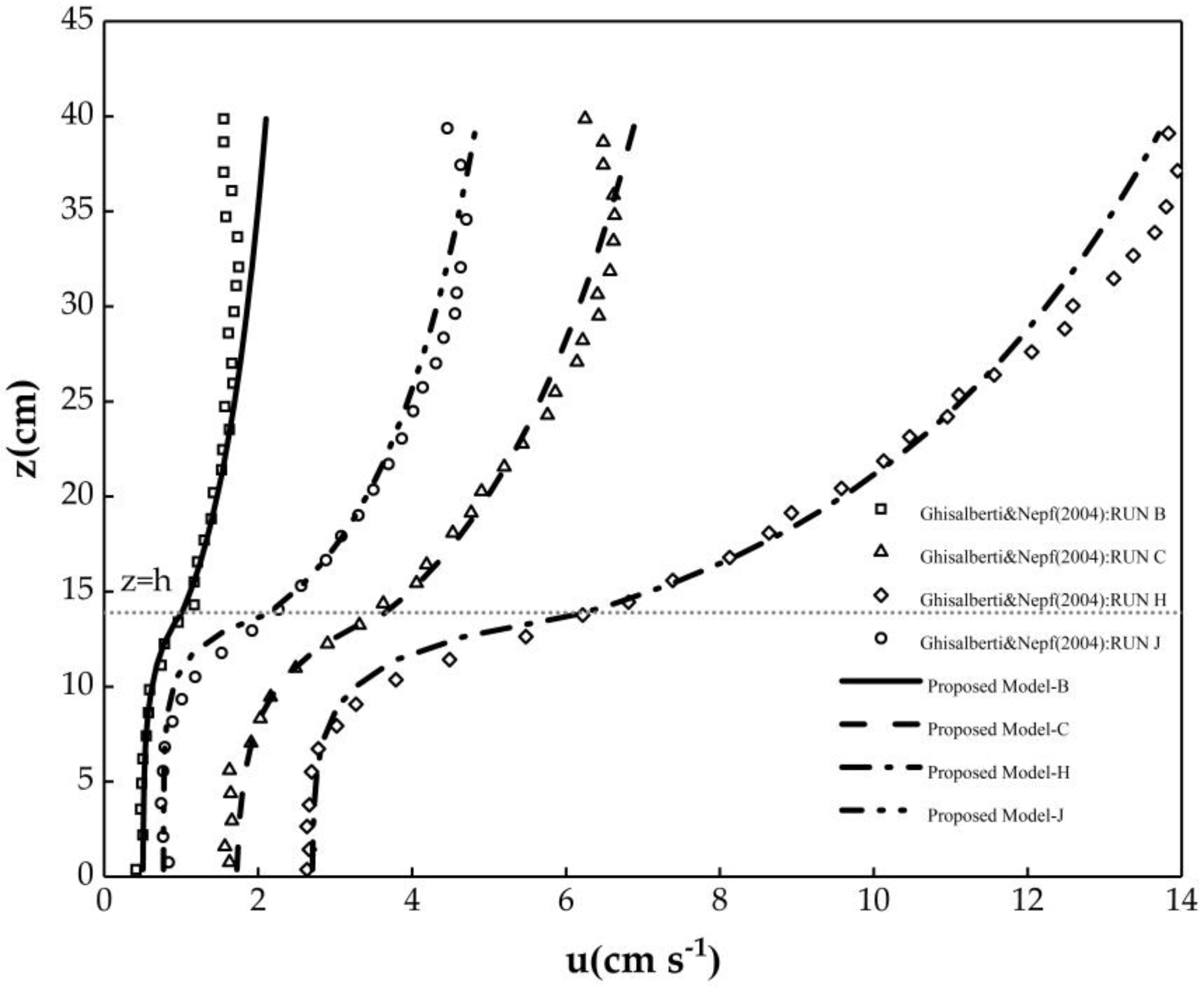
To verify the flow model of Equations (6) and (9), we collected data from Ghisalberti and Nepf [27]. In their experiments, a constant flow depth ($H$) of 46.7 cm was employed, with the vegetation height ($h$) of 13.9 cm or 13.8 cm. Model canopies consisted of circular wooden cylinders ($d=$ 0.64 cm) arranged randomly in holes into Plexiglas boards. The range of dimensionless plant densities ($ad=$ 0.016~0.051) is representative of dense aquatic meadows.

Table 1. Summary of experiment condition parameters in Ghisalberti and Nepf [27].

RUN	Q, ×10−2 cm3 s−1	h, cm	a, cm−1	S, ×10−5	u1, cm s−1	uh, cm s−1
A	48	13.9	0.025	0.99	1.30	2.50
B	17	13.9	0.025	0.18	0.50	1.00
C	74	13.9	0.034	2.50	1.70	3.50
D	48	13.9	0.034	1.20	1.10	2.40
E	143	13.8	0.040	7.50	3.50	6.70
F	94	13.8	0.040	3.20	2.40	4.60
G	48	13.8	0.040	1.30	1.10	2.30
H	143	13.8	0.080	10.00	2.70	6.30
I	94	13.8	0.080	3.40	1.70	4.00
J	48	13.8	0.080	1.30	0.77	2.10
K	17	13.8	0.080	0.26	0.27	0.94

details the relevant flow parameters.

Figure 3 shows the vertical distribution of the mean longitudinal velocity from the bed to the water surface. Inside the canopy, the velocity profile predicted by Equation (9) agrees well with the experimental data of Ghisalberti and Nepf [27]. In the free water layer, the velocity profile predicted by Equation (6) is in moderate agreement with the measured data. However, the predicted mean velocity near the free surface deviates significantly from the observations. This result is due to the velocity dip caused by the small width-to-depth ratio used in their experiments [8].

3.2. Verification of Suspended Sediment Concentration Model

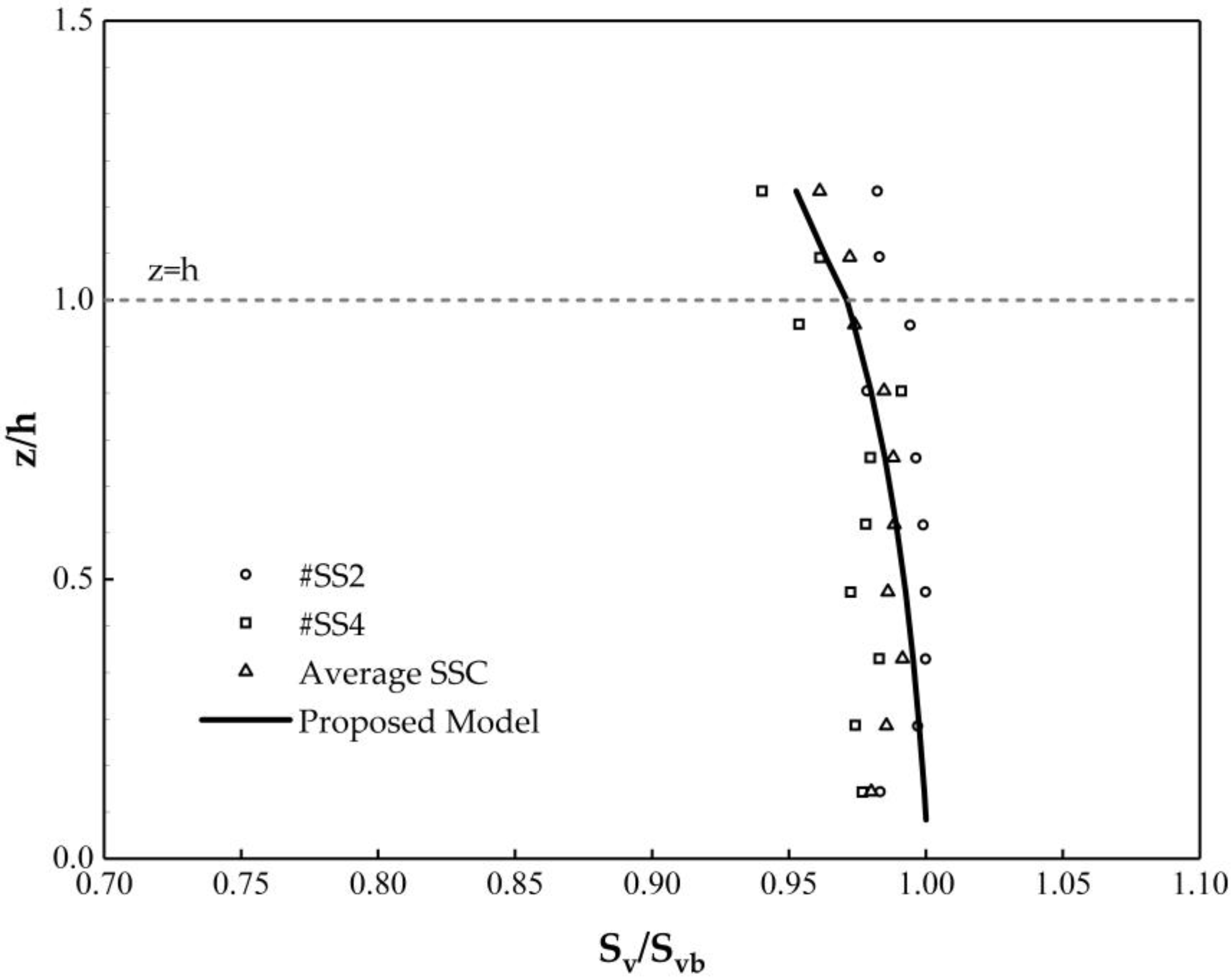
The model of suspended sediment concentration is verified by the experimental data measured by Wang et al., who conducted experiments in flume with flexible submerged canopies [28]. Their flume was 33.0 m long, 0.50 m wide, and 0.50 m deep. The flow depth in the experiment was 35 cm. The canopy used in their experiment was bent by flow, and the deflected height in water was 25.1 cm in average. The frontal area per canopy volume ($a$) was 0.009 cm⁻¹, and the mean diameter of sediment was 11.38 μm, with the fall velocity $\omega =$ 0.009 cm/s. Figure 4 presents the vertical distribution of suspended sediment concentration predicted by Equations (16) and (17). The results are compared with the experiment data. #SS2 and #SS4 are two sampling positions in one experiment. Therefore, we averaged the two sets of data, considering the deviation in experiments. The predicted profile moderately agrees with the averaged data. However, a deviation remains between the predicted profile and the measured data near the bed. Inferring from previous studies, a large concentration of suspended sediment exists when the spatial position is lower. The predicted profile conforms to the law while the measured profile failed. Neglecting the experiment error, the deviation may be caused by the inhomogeneity of the natural vegetation used in the experiment, which enhanced the complexity of the hydrodynamic conditions.

3.3. Sensitivity Analysis of Canopy Density

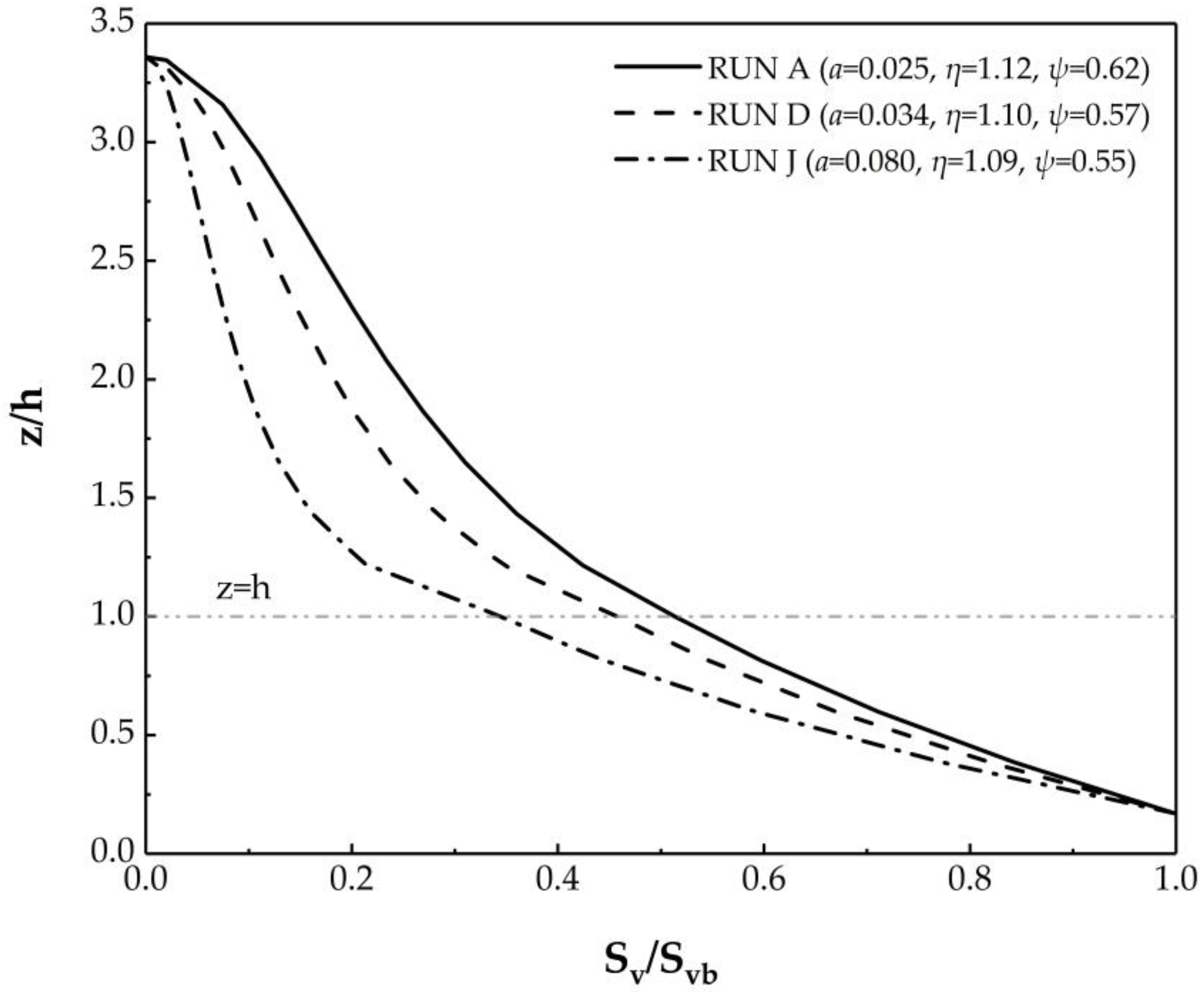
The canopy density is an important factor determining canopy flow. It exerts great influence on the velocity profile, which affects the vertical distribution of suspended sediment concentration. To investigate the effects of canopy density, we assumed the submerged canopy flow with sediment particles ($d_{50}=0.005\mathrm{cm}$) under the hydrodynamic in Table 1 for Runs A, D, and J. These three sets of experiments have the same flow depth, discharge, and canopy height but different canopy densities. Therefore, the bed slope ($S$) was adjusted to form the uniform flow. Table 1 shows that that the bed slope increases with increasing canopy density. Meanwhile, the suspension index ($\psi$) decreases with increasing bed slope under the same sediment particle settling velocity.

Table 2. Parameters are used in the following analysis under the hydrodynamic in Table 1.

RUN	${\mathit{u}}_{\ast }$, cm s−1	$\mathit{\omega }$, cm s−1	$\mathit{\eta }$	$\mathit{\psi }$
A	0.56	0.16	1.12	0.62
B	0.24	0.16	1.66	0.98
C	0.90	0.16	1.05	0.42
D	0.62	0.16	1.10	0.57
E	1.56	0.16	1.02	0.25
F	1.02	0.16	1.04	0.37
G	0.65	0.16	1.09	0.55
H	1.80	0.16	1.01	0.21
I	1.05	0.16	1.03	0.36
J	0.65	0.16	1.09	0.55
K	0.29	0.16	1.45	0.93

details the parameters which will be used in the following analysis. The friction velocity is calculated by Equation (7) and the inverse of turbulent Schmidt number is calculated by Equation (3).

Figure 5 shows the vertical distribution profile of the suspended sediment concentration predicted by Equations (16) and (17). Obviously, the greater the canopy density, the more uneven the vertical distribution of suspended sediment concentration. In addition, the proportion of suspended sediment concentration above the canopy layer gradually decreases. Thus, the canopy layer can capture more sediment particles when the density of vegetation is greater. The main reason is that the greater canopy density increases the resistance and decreases the average flow velocity. It makes the gravity effect of sediment particles stronger than the turbulence effect. Thus, the sediment is deposited into the canopy layer.

3.4. Sensitivity Analysis of Hydraulic Condition

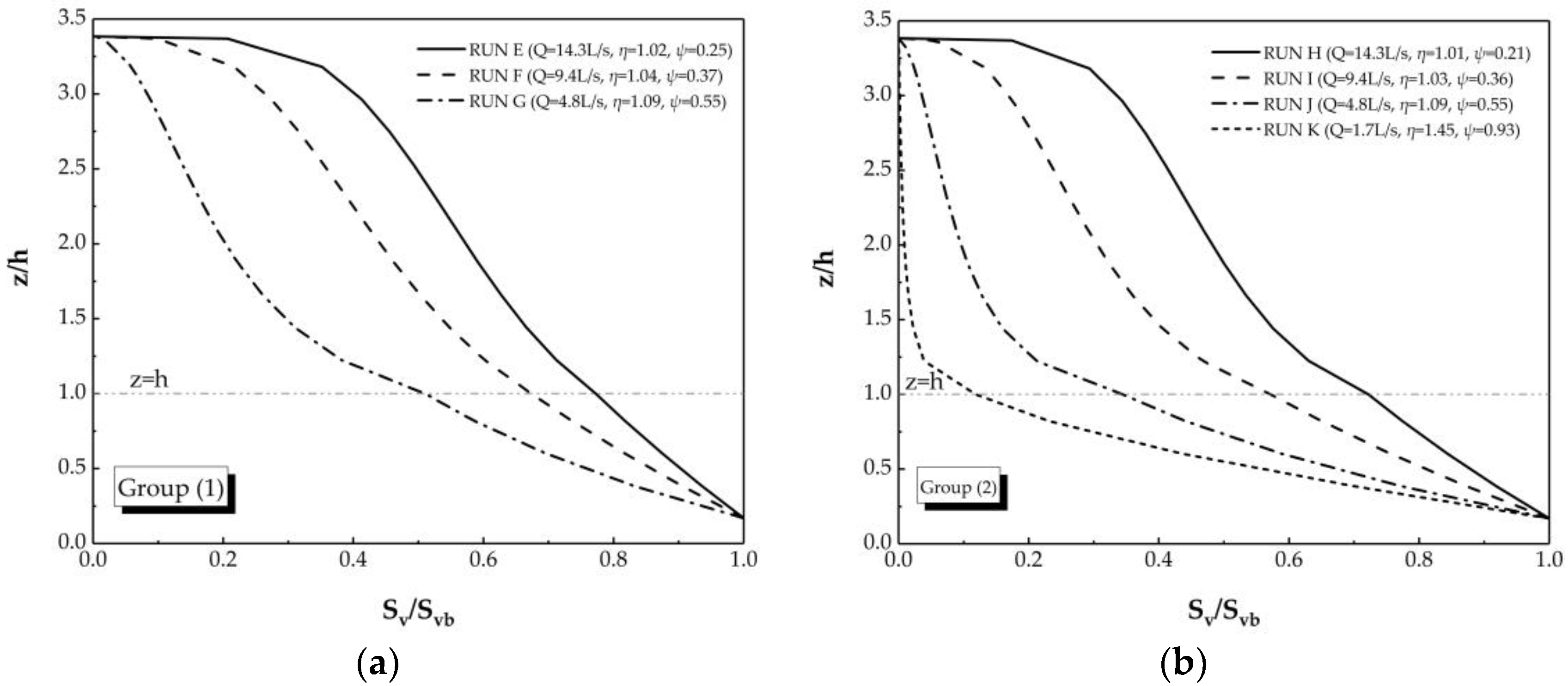
A vegetation area with determined canopy density is often subject to different hydraulic conditions. To find the influence of hydraulic condition, we assumed the submerged canopy sediment-laden flow under the hydrodynamic conditions in Table 1 for Runs E, F, G, H, I, J, and K. The seven sets of experiments were divided into Group (1) and Group (2). Group (1) has Runs E, F, and G with the same canopy density ($a=$ 0.040), whereas Group (2) has Runs H, I, J, and K with the same canopy density ($a=$ 0.080). Figure 6 shows the vertical distribution profile of the two groups.

For achieving uniform flow, the bed slope increases with increasing input discharge under the same discharge so that the friction velocity will also increase under the same flow depth. Therefore, greater input discharge corresponds to smaller suspension index. Figure 6 shows that the vertical distribution profile is more even with the smaller suspension index. The greater input discharge can bring more sediment particles and facilitate even distribution. The larger discharge renders the turbulence effect stronger and thus the sediment particles more suspended. Conversely, the smaller discharge increases the gravity effect and the deposition of the sediment particles. This finding is in line with our basic understanding.

The suspension index ($\psi$) in the vertical distribution law of the suspension load determines the uniformity of the sediment on the vertical line. The smaller the suspension index, the more uniform the distribution of the suspended load. The results in Figure 6 agree with this rule, whereas those in Figure 5 disagree. The situation reveals that the vertical distribution profile is heavily affected by the canopy density. In addition, for a determined canopy density, the uniformity is controlled by the suspension index.

3.5. Sensitivity Analysis of the Inverse of Turbulent Schmidt Number

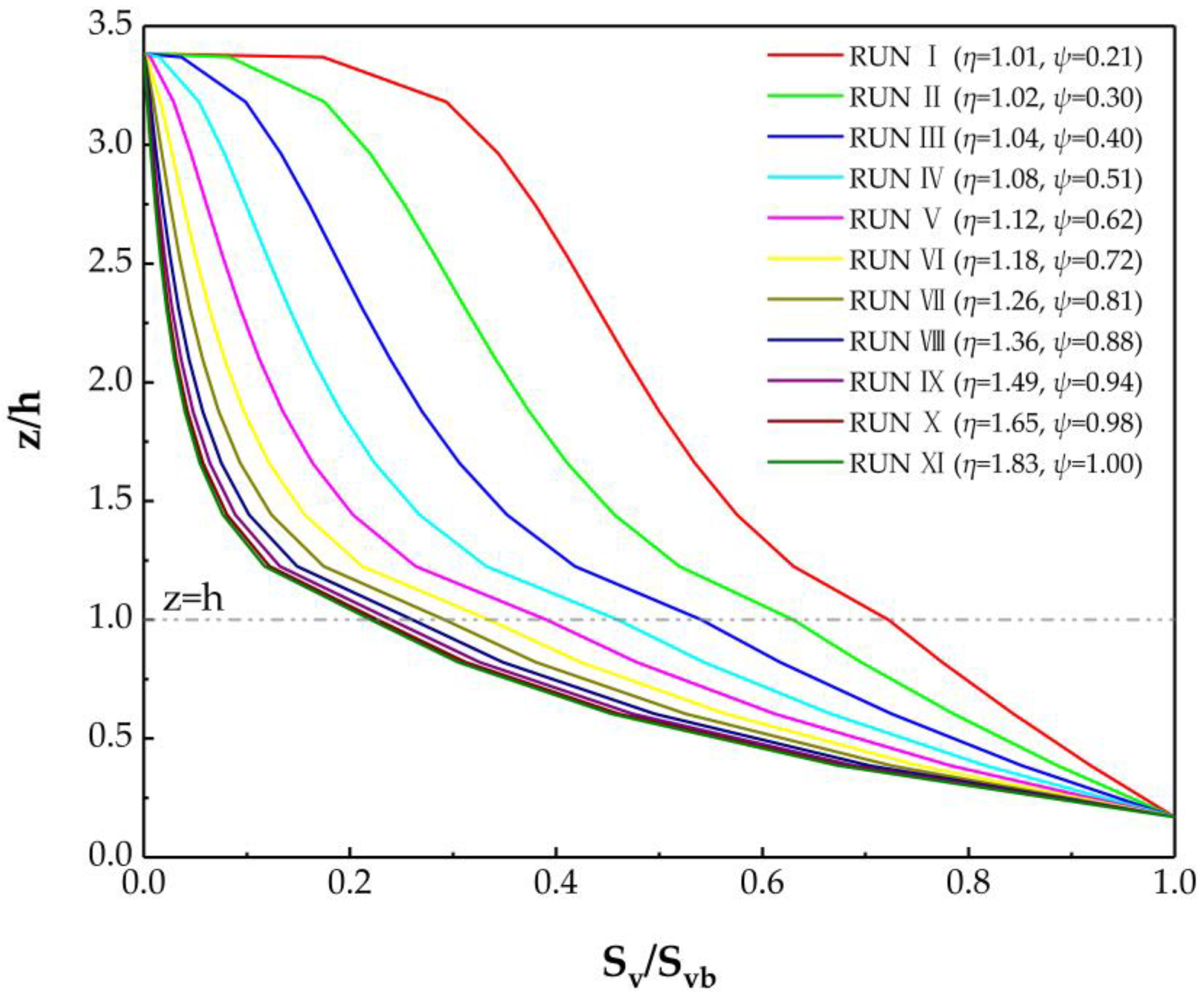
The inverse of turbulent Schmidt number or the parameter $\eta$ has great influence on the suspended sediment concentration profile. To investigate the effect of the parameter $\eta$, the submerged canopy flows containing different median particle size ($d_{50}$) were assumed under the same hydrodynamic condition (Run H in Table 1). The relevant calculation parameters are presented in

Table 3. The relevant calculation parameters for analyzing the influence of the parameter $\eta$.

RUN	${\mathit{d}}_{50}$, cm	$\mathit{\omega }$, cm s−1	${\mathit{u}}_{\ast }$, cm s−1	$\mathit{\eta }$	$\mathit{\psi }$
I	0.005	0.16	1.80	1.01	0.21
II	0.006	0.22	1.80	1.02	0.30
III	0.007	0.30	1.80	1.04	0.40
IV	0.008	0.40	1.80	1.08	0.51
V	0.009	0.50	1.80	1.12	0.62
VI	0.010	0.61	1.80	1.18	0.72
VII	0.011	0.74	1.80	1.26	0.81
VIII	0.012	0.87	1.80	1.36	0.88
IX	0.013	1.01	1.80	1.49	0.94
X	0.014	1.16	1.80	1.65	0.98
XI	0.015	1.32	1.80	1.83	1.00

.

.

Figure 7 presents the proposed vertical distribution profile of the eleven runs. According to Equation (3), it can be known that the parameter $\eta$ increases with the settling velocity under the same hydrodynamic condition, while the Rouse number ($\psi$) also increases. Observing from Figure 7, it can be found that the suspended sediment distribution profile becomes more and more non-uniform from Run I to Run XI. However, the changing range of the vertical distribution profile gradually gets smaller. That indicates the increasing inverse of turbulent Schmidt number or the parameter $\eta$ gradually has less impact on the particle concentration profile.

4. Conclusions

A model to describe the vertical distribution of the diffusion coefficient in a flow with submerged canopies was presented. The diffusion coefficient (${\epsilon }_z$) has different distributions in the canopy layer and the free water layer. The diffusion coefficient follows a linear distribution above the canopy height while an exponential profile inside the canopy layer. Expressions for the vertical distribution profile of suspended sediment concentration were then derived. The verification result reveals that the model moderately agrees with the experimental data.

Sensitivity analysis was performed for canopy density, hydraulic conditions and turbulent Schmidt number. Under the same hydrodynamic conditions, the vertical distribution becomes more uneven with increasing canopy density. Greater canopy density corresponds to more sediment particles in the vegetation layer. For a determined canopy density, the hydraulic conditions mainly change the suspension index, i.e., it increases with the increasing discharge. In addition, the vertical distribution becomes less uniform. It meets the vertical distribution law of the suspension load, as confirmed by Rouse formula. The parameter $\eta$ has great influence on the vertical distribution profile. The distribution of suspended sediment concentration becomes uneven with a larger $\eta$. However, the variation of the vertical distribution of suspended sediment gradually becomes smaller with the increasing parameter $\eta$.

For practical purposes, further research should focus on the effect of the depth ratio and the different canopy characteristics. Additional experiments are also needed to determine the application scope of the model and verify the effects of the canopy density. Furthermore, the relationship between the sediment diffusion coefficient and momentum diffusion coefficient adopted in this study is investigated in the open-channel flow without vegetation. Therefore, the influence of vegetation on the relationship can be further studied.

References

- Graf, W.H. Hydraulics of Sediment Transport; McGraw-Hill: New York, NY, USA, 1971; Volume 172. [Google Scholar]
- Tisujimoto, T. Diffusion coefficient of suspended sediment and kinematic eddy viscosity of flow containing suspended load. In River Flow 2010; Koll, D., Geisenhainer, A., Eds.; Bundesanstalt für Wasserbau: Karlsruhe, Germany, 2010; pp. 801–806. ISBN 978-3-939230-00-7. [Google Scholar]
- Pal, D.; Ghoshal, K. Effect of particle concentration on sediment and turbulent diffusion coefficients in open-channel turbulent flow. Environ. Earth Sci. 2016, 75, 1245. [Google Scholar] [CrossRef]
- Gualtieri, C.; Angeloudis, A.; Bombardelli, F.; Jha, S.; Stoesser, T. On the values for the turbulent Schmidt number in environmental flows. Fluids 2017, 2, 17. [Google Scholar] [CrossRef]
- Van Rijin, L.C. Sediment transport, part ii: Suspended load transport. J. Hydraul. Eng. 1984, 110, 1613–1641. [Google Scholar] [CrossRef]
- Graf, W.H.; Cellino, M. Suspension flows in open channels: Experimental study. J. Hydraul. Res. 2002, 40, 435–447. [Google Scholar] [CrossRef]
- Rouse, H. Experiments on the mechanics of sediment suspension. In Proceedings of the Fifth International Congress for Applied Mechanics, Cambridge, MA, USA, 12–16 September 1938; John Wiley & Sons: New York, NY, USA, 1938; pp. 550–554. [Google Scholar]
- Yang, W.; Choi, S.U. A two-layer approach for depth-limited open channel flows with submerged vegetation. J. Hydraul. Res. 2010, 48, 466–475. [Google Scholar] [CrossRef]
- Klopstra, D.; Barneveld, H.J.; Van Noortwijk, J.M.; Van Velzen, E.H. Analytical model for hydraulic roughness of submerged vegetation. In Proceedings of the 27th Congress of the International Association for Hydraulic Research, San Francisco, CA, USA, 10–15 August 1997; pp. 775–780. [Google Scholar]
- Huai, W.X.; Zeng, Y.H.; Xu, Z.G.; Yang, Z.H. Three-layer model for vertical velocity distribution in open channel flow with submerged rigid vegetation. Adv. Water Resour. 2009, 32, 487–492. [Google Scholar] [CrossRef]
- Follett, E.; Chamecki, M.; Nepf, H. Evaluation of a random displacement model for predicting particle escape from canopies using a simple eddy diffusivity model. Agric. For. Meteorol. 2016, 224, 40–48. [Google Scholar] [CrossRef] [Green Version]
- De Serio, F.; Ben Meftah, M.; Mossa, M.; Termini, D. Experimental investigation on dispersion mechanisms in rigid and flexible vegetated bed. Adv. Water Resour. 2018, 120, 98–113. [Google Scholar] [CrossRef]
- Nepf, H.M. Flow and transport in regions with aquatic vegetation. Annu. Rev. Fluid Mech. 2012, 44, 123–142. [Google Scholar] [CrossRef]
- Nepf, H.; Ghisalberti, M.; White, B.; Murphy, E. Retention time and dispersion associated with submerged aquatic canopies. Water Resour. Res. 2007, 43, W04422. [Google Scholar] [CrossRef]
- Liu, X.G.; Zeng, Y.H. Drag coefficient for rigid vegetation in subcritical open-channel flow. Environ. Fluid Mech. 2017, 17, 1035–1050. [Google Scholar] [CrossRef]
- Kaimal, J.; Finnigan, J. Atmospheric Boundary Layer Flows: Their Structure and Measurement, 1st ed.; Oxfod University Press: New York, NY, USA, 1994; Volume 289. [Google Scholar]
- Murphy, E.; Ghisalberti, M.; Nepf, H. Model and laboratory study of dispersion in flows with submerged vegetation. Water Resour. Res. 2007, 43, W05438. [Google Scholar] [CrossRef]
- Järvelä, J. Effect of submerged flexible vegetation on flow structure and resistance. J. Hydrol. 2005, 307, 233–241. [Google Scholar] [CrossRef]
- Nepf, H.M.; Vivoni, E.R. Flow structure in depth-limited, vegetated flow. J. Geophys. Res-Oceans 2000, 105, 28547–28557. [Google Scholar] [CrossRef] [Green Version]
- Thom, A.S. Momentum absorption by vegetation. Q. J. R. Meteorol. Soc. 2010, 97, 414–428. [Google Scholar] [CrossRef]
- Luhar, M.; Rominger, J.; Nepf, H. Interaction between flow, transport and vegetation spatial structure. Environ. Fluid Mech. 2008, 8, 423–439. [Google Scholar] [CrossRef]
- Raupach, M.R.; Thom, A.S.; Edwards, I. A wind-tunnel study of turbulent flow close to regularly arrayed rough surfaces. Bound. Layer Meteorol. 1980, 18, 373–397. [Google Scholar] [CrossRef]
- Harman, I.N.; Finnigan, J.J. A simple unified theory for flow in the canopy and roughness sublayer. Bound. Layer Meteorol. 2007, 123, 339–363. [Google Scholar] [CrossRef]
- Shimizu, Y.; Tsujimoto, T.; Nakagawa, H.; Kitamura, T. Experimental study on flow over rigid vegetation simulated by cylinders with equi-spacing. Proc. JSCE 2010, 1991, 31–40. (In Japanese) [Google Scholar]
- Dijkstra, J.T.; Uittenbogaard, R.E. Modeling the interaction between flow and highly flexible aquatic vegetation. Water Resour. Res. 2010, 46, W12547. [Google Scholar] [CrossRef]
- Huai, W.X.; Wang, W.J.; Zeng, Y.H. Two-layer model for open channel flow with submerged flexible vegetation. J. Hydraul. Res. 2013, 51, 708–718. [Google Scholar] [CrossRef]
- Ghisalberti, M.; Nepf, H. The limited growth of vegetated shear layers. Water Resour. Res. 2004, 40, W07502. [Google Scholar] [CrossRef]
- Wang, X.Y.; Xie, W.M.; Zhang, D.; He, Q. Wave and vegetation effects on flow and suspended sediment characteristics: A flume study. Estura. Coast. Shelf Sci. 2016, 182, 1–11. [Google Scholar] [CrossRef]
Figure 1.
Cross-section of a vegetated channel.
Figure 2.
Schematic of the time-averaged longitudinal velocity () model.
Figure 3.
Vertical distribution of mean velocity in the whole flow depth.
Figure 4.
Vertical distribution of suspended sediment concentration compared with experimental data measured by Wang et al. [28].
Figure 5.
Vertical distribution of suspended sediment concentration for Runs A, D and J.
Figure 6.
Vertical distribution of suspended sediment concentration for sensitivity analysis of hydraulic conditions. (a) Group (1); (b) Group (2).
Figure 7.
Vertical distribution profile of suspended sediment concentration for sensitivity analysis of the parameter .