The Use of River Flow Discharge and Sediment Load for Multi-Objective Calibration of SWAT Based on the Bayesian Inference

 , , , and
Abstract
:1. Introduction
2. Study Area
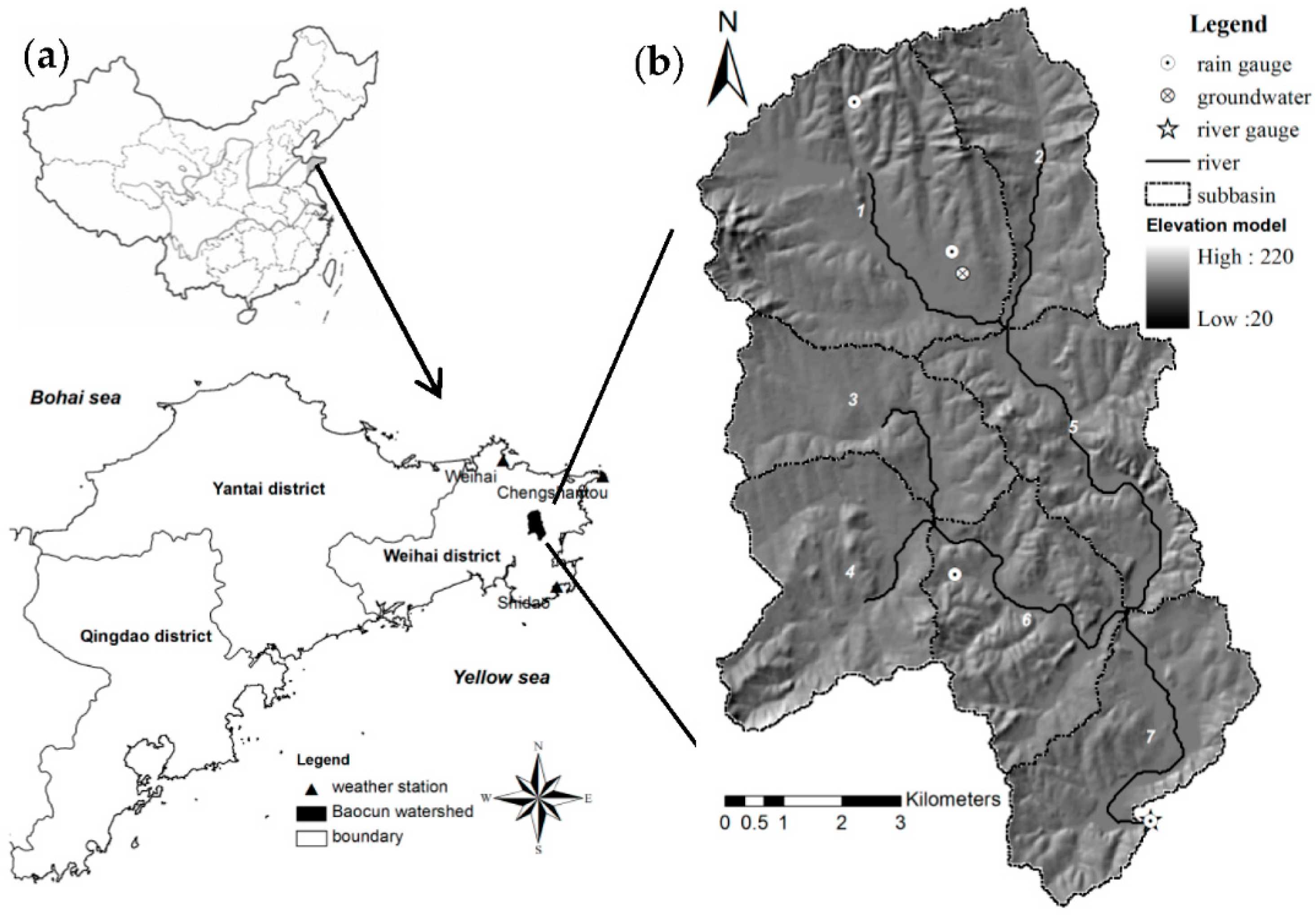
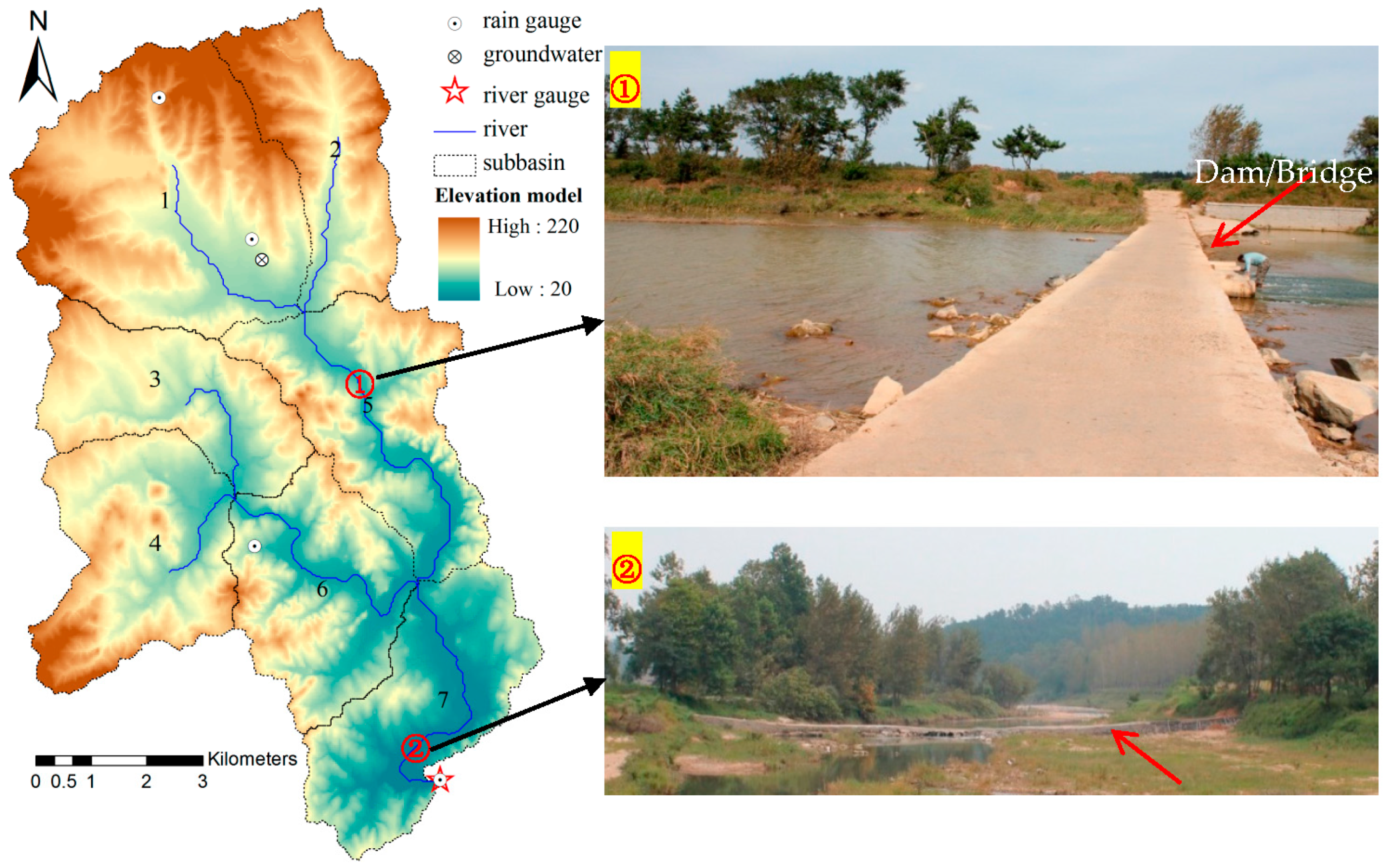
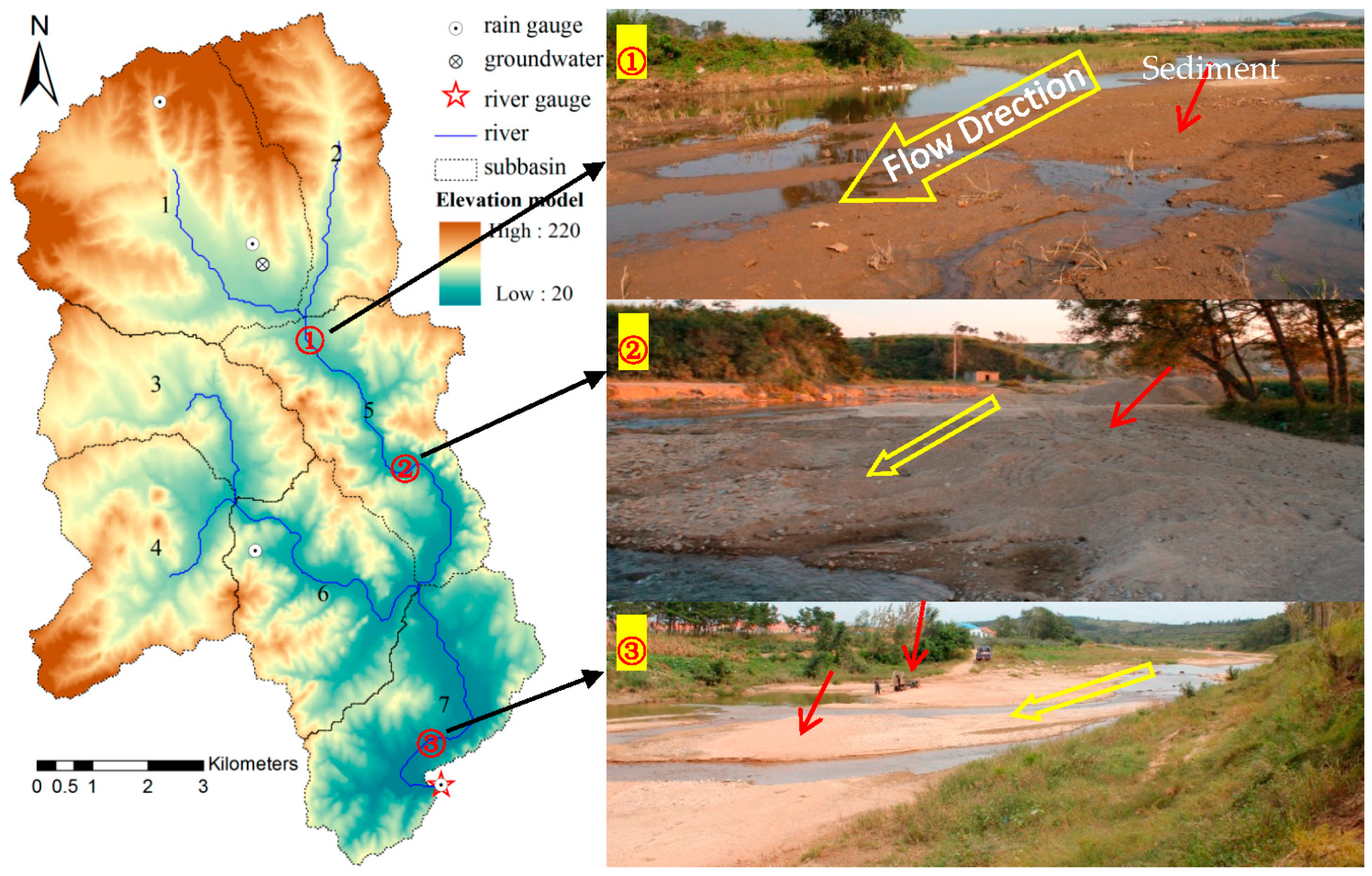
2.1. Baocun Watershed
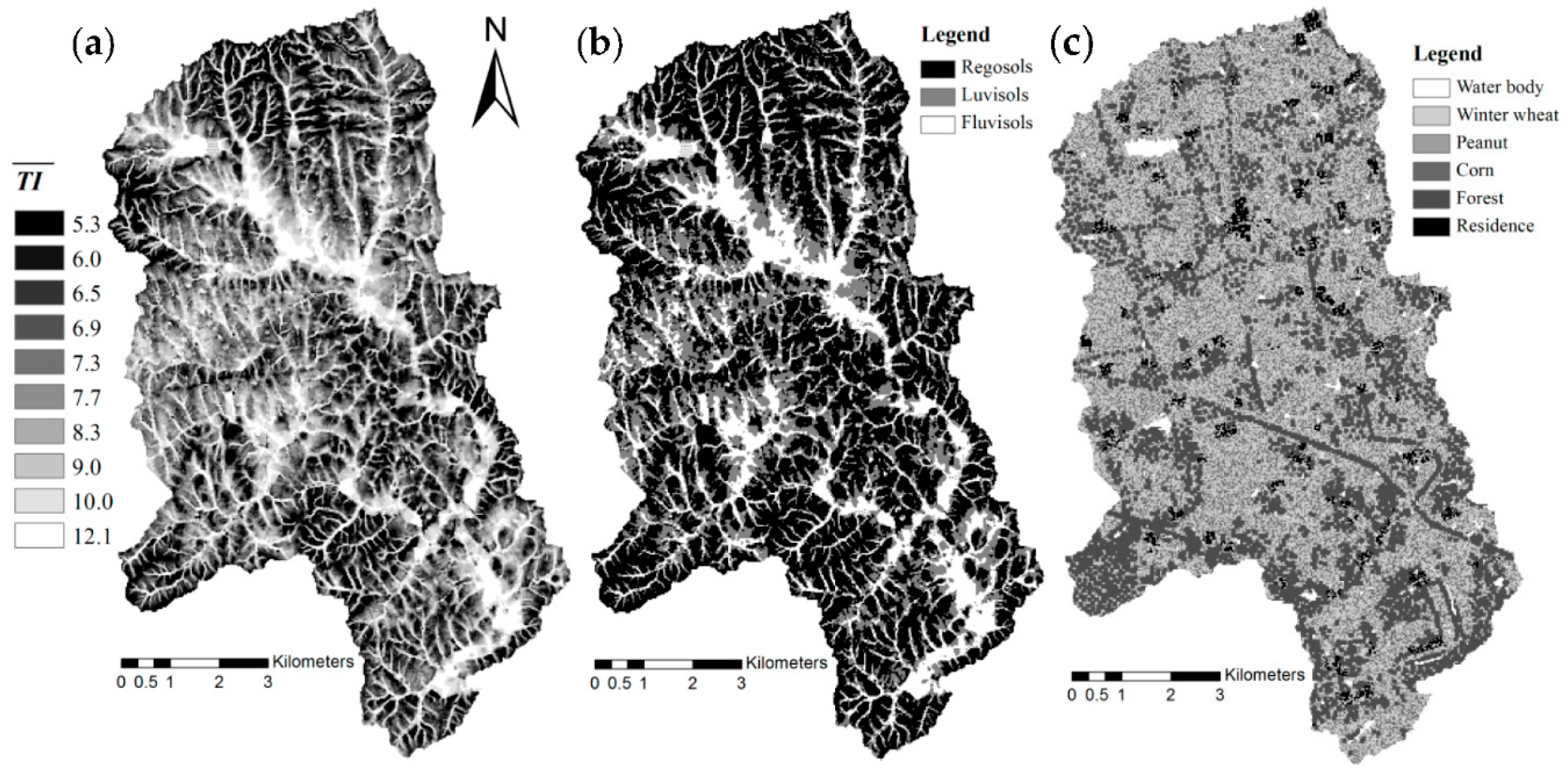
2.2. Model Input Data
3. Methods
3.1. SWAT-WB-VSA Model
3.1.1. Surface Runoff Generation
3.1.2. Sediment
3.2. Model Calibration
3.3. Transformation of Flow and Sediment Objectives to a Likelihood Function
3.3.1. Case with NSE
3.3.2. Case with BC-GED
4. Results
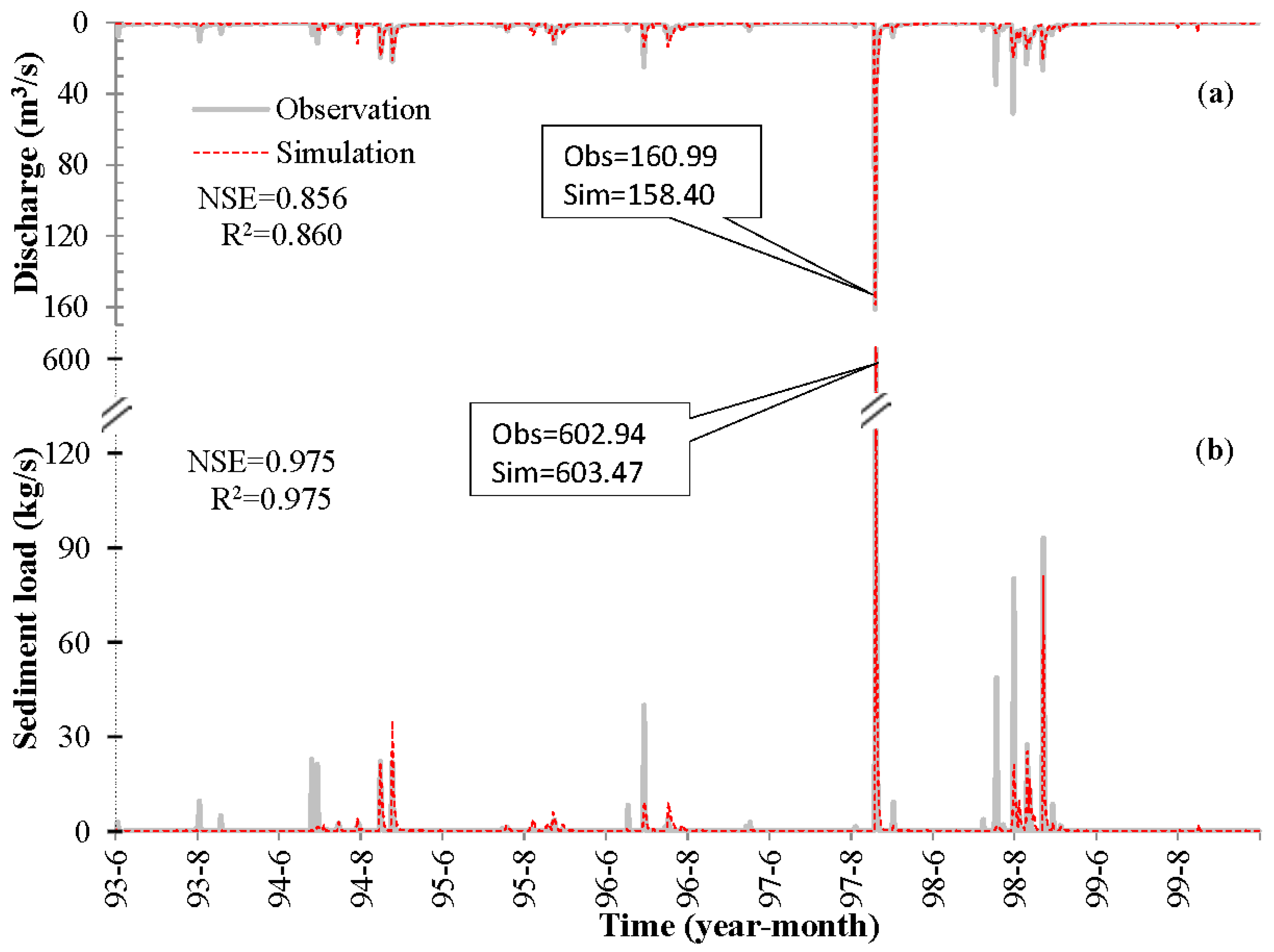
4.1. NSE Approach
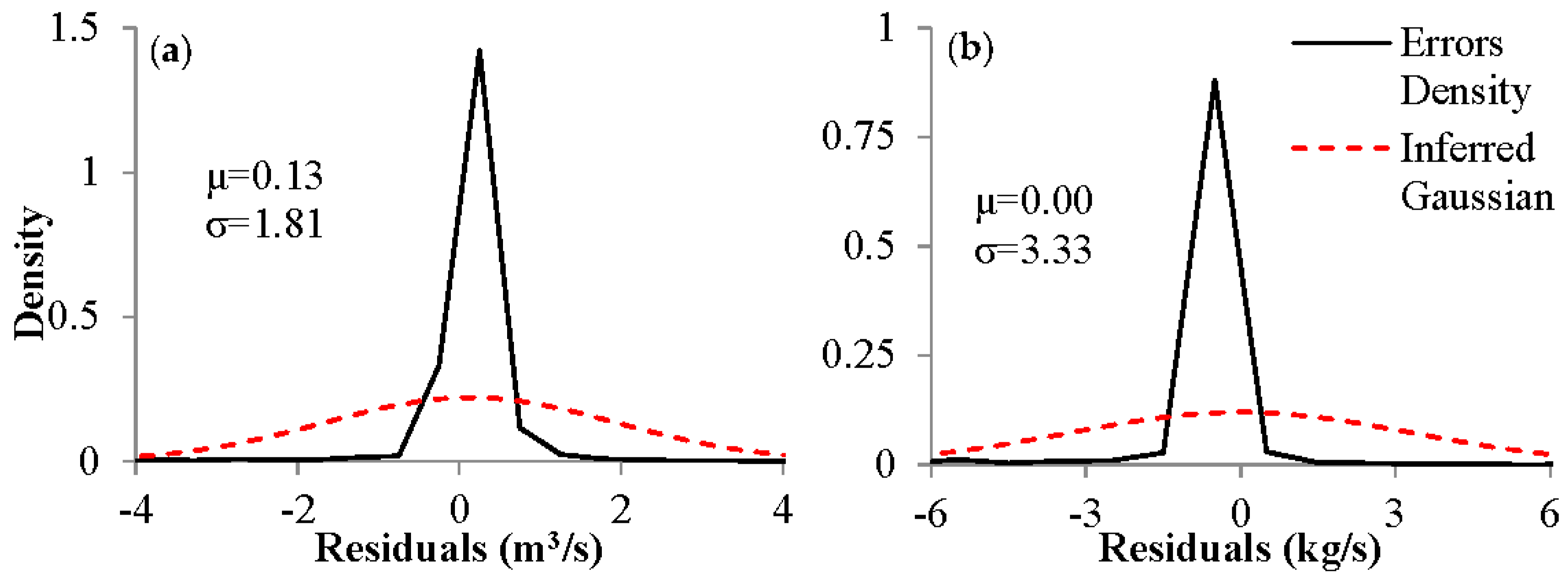
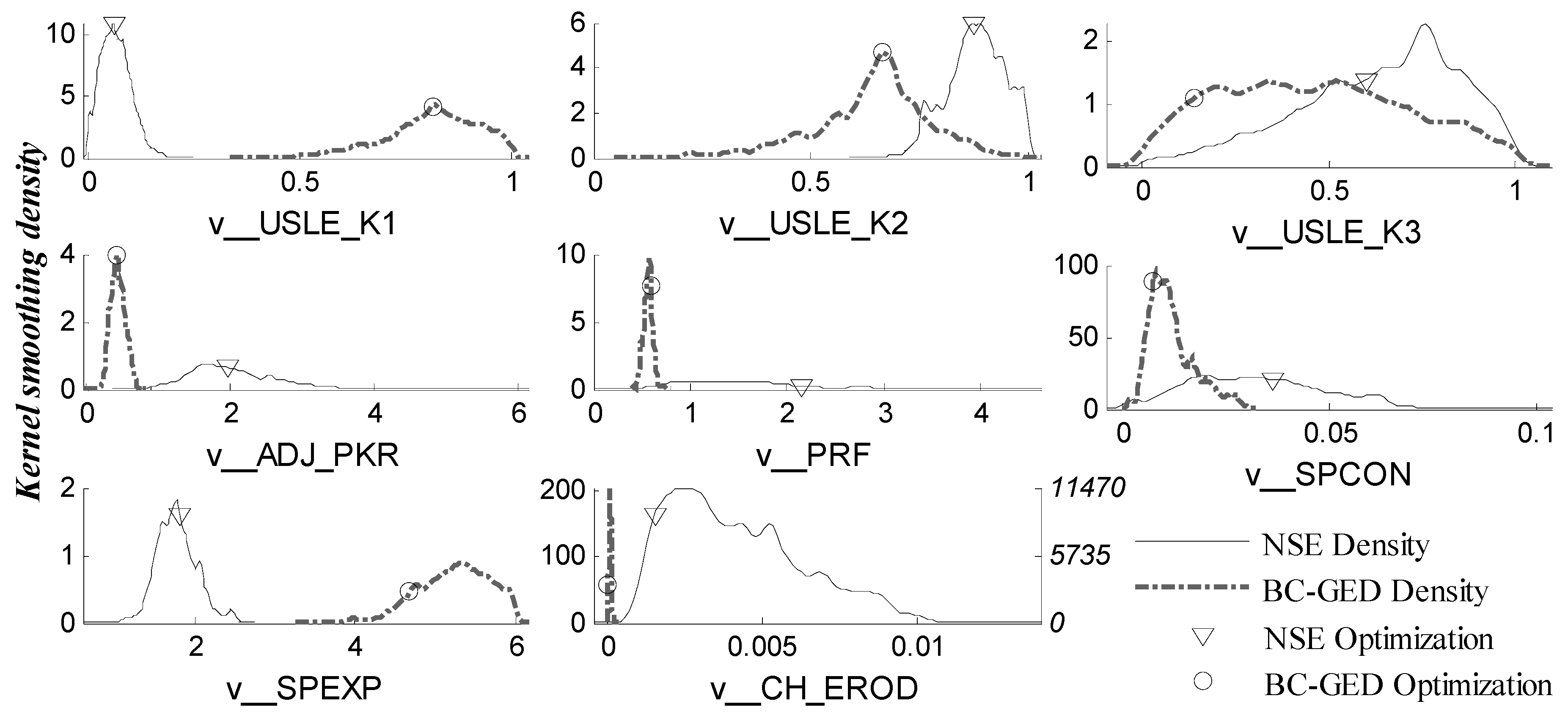
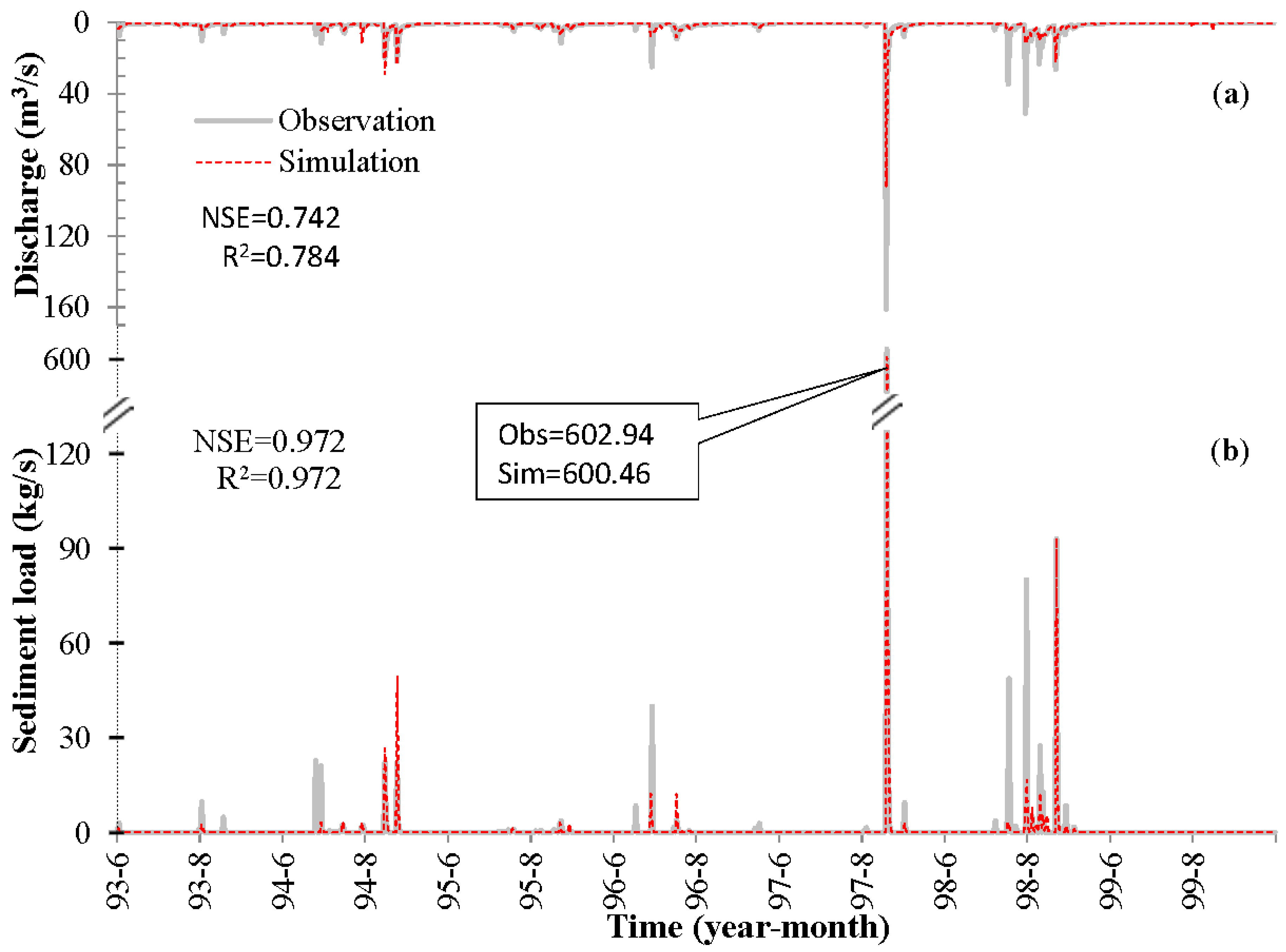
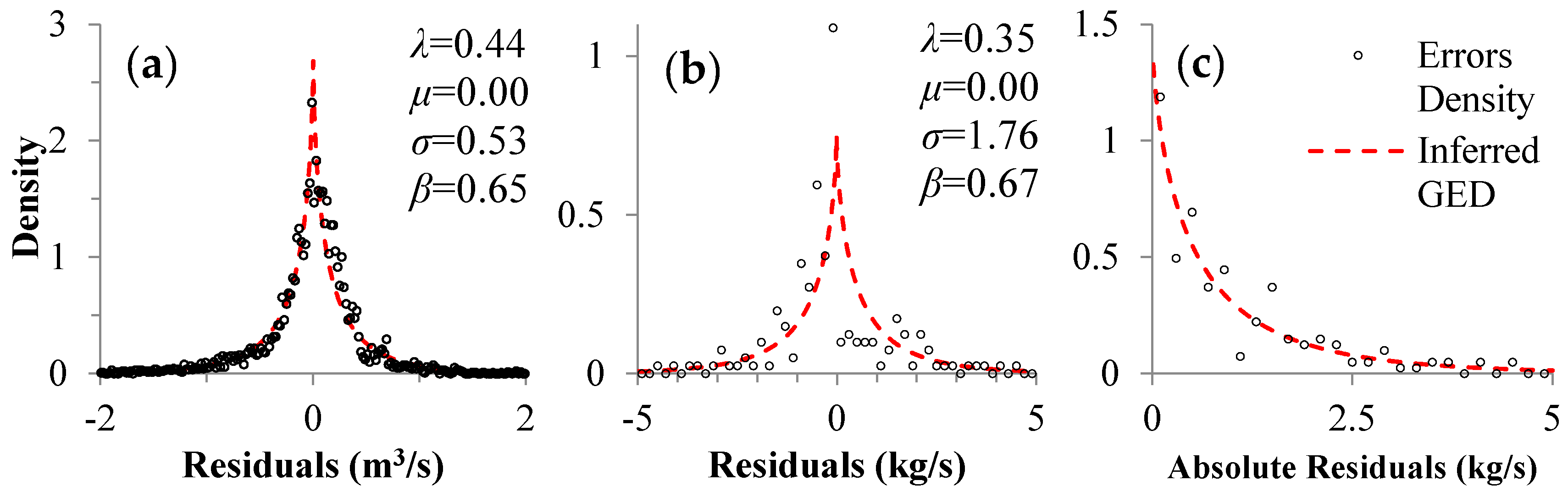
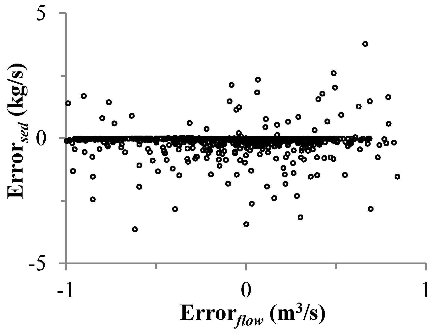
4.2. BC-GED Approach
5. Discussion
5.1. Effects of Multi-Objective Approach
5.2. Difference between NSE and BC-GED Error Model
6. Conclusions
Author Contributions
Funding
Acknowledgments
Conflicts of Interest
References
- Gassman, P.W.; Reyes, M.R.; Green, C.H.; Arnold, J.G. The Soil and Water Assessment Tool: Historical Development, Applications, and Future Research Directions. Trans. ASABE 2007, 50, 1211–1250. [Google Scholar] [CrossRef] [Green Version]
- Cheng, Q.-B.; Reinhardt-Imjela, C.; Chen, X.; Schulte, A.; Ji, X.; Li, F. Improvement and comparison of the rainfall-runoff methods in SWAT at the monsoonal watershed of Baocun, Eastern China. Hydrol. Sci. J. 2016, 61, 1460–1476. [Google Scholar] [CrossRef]
- Williams, J.R. Chapter 25: The EPIC model. In Computer Models of Watershed Hydrology; Singh, V.P., Ed.; Water Resources Publications: Highlands Ranch, CO, USA, 1995; pp. 909–1000. [Google Scholar]
- Bagnold, R.A. Bed load transport by natural rivers. Water Resour. Res. 1977, 13, 303–312. [Google Scholar] [CrossRef]
- Williams, J.R. SPNM, a Model for Predicting Sediment, Phosphorus, and Nitrogen Yields from Agricultural Basins. J. Am. Water Resour. Assoc. 1980, 16, 843–848. [Google Scholar] [CrossRef]
- Gebremicael, T.G.; Mohamed, Y.A.; Betrie, G.D.; van der Zaag, P.; Teferi, E. Trend analysis of runoff and sediment fluxes in the Upper Blue Nile basin: A combined analysis of statistical tests, physically-based models and landuse maps. J. Hydrol. 2013, 482, 57–68. [Google Scholar] [CrossRef]
- Arnold, J.G.; Moriasi, D.N.; Gassman, P.W.; Abbaspour, K.C.; White, M.J.; Srinivasan, R.; Santhi, C.; Harmel, R.D.; Griensven, A.V.; Liew, M.W.V. SWAT: Model use, calibration, and validation. Trans. ASABE 2012, 55, 1345–1352. [Google Scholar] [CrossRef]
- Lu, S.; Kayastha, N.; Thodsen, H.; Van, G.A.; Andersen, H.E. Multiobjective calibration for comparing channel sediment routing models in the soil and water assessment tool. J. Environ. Qual. 2014, 43, 110–120. [Google Scholar] [CrossRef] [PubMed]
- Gupta, H.V.; Sorooshian, S.; Yapo, P.O. Toward improved calibration of hydrologic models: Multiple and noncommensurable measures of information. Water Resour. Res. 1998, 34, 751–763. [Google Scholar] [CrossRef] [Green Version]
- Efstratiadis, A.; Koutsoyiannis, D. One decade of multi-objective calibration approaches in hydrological modelling: A review. Hydrol. Sci. J. 2010, 55, 58–78. [Google Scholar] [CrossRef]
- Abbaspour, K.C.; Yang, J.; Maximov, I.; Siber, R.; Bogner, K.; Mieleitner, J.; Zobrist, J.; Srinivasan, R. Modelling hydrology and water quality in the pre-alpine/alpine Thur watershed using SWAT. J. Hydrol. 2007, 333, 413–430. [Google Scholar] [CrossRef]
- Wang, Y.; Brubaker, K. Multi-objective model auto-calibration and reduced parameterization: Exploiting gradient-based optimization tool for a hydrologic model. Environ. Model. Softw. 2015, 70, 1–15. [Google Scholar] [CrossRef]
- Bekele, E.G.; Nicklow, J.W. Multi-objective automatic calibration of SWAT using NSGA-II. J. Hydrol. 2007, 341, 165–176. [Google Scholar] [CrossRef]
- Vrugt, J.A.; Gupta, H.V.; Bastidas, L.A.; Bouten, W.; Sorooshian, S. Effective and efficient algorithm for multiobjective optimization of hydrologic models. Water Resour. Res. 2003, 39, 1214. [Google Scholar] [CrossRef]
- Deb, K.; Pratap, A.; Agarwal, S.; Meyarivan, T. A fast and elitist multiobjective genetic algorithm: NSGA-II. IEEE Trans. Evol. Comput. 2002, 6, 182–197. [Google Scholar] [CrossRef] [Green Version]
- Vrugt, J.A.; Robinson, B.A. Improved evolutionary optimization from genetically adaptive multimethod search. Proc. Natl. Acad. Sci. USA 2007, 104, 708–711. [Google Scholar] [CrossRef] [PubMed] [Green Version]
- Huang, Y. Multi-objective calibration of a reservoir water quality model in aggregation and non-dominated sorting approaches. J. Hydrol. 2014, 510, 280–292. [Google Scholar] [CrossRef]
- Reichert, P.; Schuwirth, N. Linking statistical bias description to multiobjective model calibration. Water Resour. Res. 2012, 48, 184–189. [Google Scholar] [CrossRef]
- Cheng, Q.B.; Chen, X.; Cheng, D.D.; Wu, Y.Y.; Xie, Y.Y. Improved Inverse Modeling by Separating Model Structural and Observational Errors. Water 2018, 10, 1151. [Google Scholar] [CrossRef]
- Li, B.; Liang, Z.; He, Y.; Hu, L.; Zhao, W.; Acharya, K. Comparison of parameter uncertainty analysis techniques for a TOPMODEL application. Stoch. Environ. Res. Risk Assess. 2017, 31, 1045–1059. [Google Scholar] [CrossRef]
- Tang, Y.; Marshall, L.; Sharma, A.; Ajami, H. A Bayesian alternative for multi-objective ecohydrological model specification. J. Hydrol. 2018, 556, 25–38. [Google Scholar] [CrossRef]
- Cheng, Q.; Chen, X.; Xu, C.; Reinhardt-Imjela, C.; Schulte, A. Improvement and comparison of likelihood functions for model calibration and parameter uncertainty analysis within a Markov chain Monte Carlo scheme. J. Hydrol. 2014, 519, 2202–2214. [Google Scholar] [CrossRef]
- Cheng, Q.; Chen, X.; Xu, C.; Zhang, Z.; Reinhardt-Imjela, C.; Schulte, A. Using maximum likelihood to derive various distance-based goodness-of-fit indicators for hydrologic modeling assessment. Stoch. Environ. Res. Risk Assess. 2018, 32, 949–966. [Google Scholar] [CrossRef]
- FAO/IIASA/ISRIC/ISSCAS/JRC. Harmonized World Soil Database, Version 1.1; FAO: Rome, Italy; IIASA: Laxenburg, Austria, 2009. [Google Scholar]
- Ministry of Water Resources of China. Code for Liquid Flow Measurement in Open Channels (GB 50179-2015); China Planning Press: Beijing, China, 2016. (In Chinese)
- Ministry of Water Resources of China. Code for Measurement of Suspended Load in Open Channels (GB/T 50159-2015); China Planning Press: Beijing, China, 2016. (In Chinese)
- White, E.D.; Easton, Z.M.; Fuka, D.R.; Collick, A.S.; Adgo, E.; McCartney, M.; Awulachew, S.B.; Selassie, Y.G.; Steenhuis, T.S. Development and application of a physically based landscape water balance in the SWAT model. Hydrol. Process. 2011, 25, 915–925. [Google Scholar] [CrossRef]
- Yustres, Á.; Asensio, L.; Alonso, J.; Navarro, V. A review of Markov Chain Monte Carlo and information theory tools for inverse problems in subsurface flow. Comput. Geosci. 2012, 16, 1–20. [Google Scholar] [CrossRef]
- Marshall, L.; Nott, D.; Sharma, A. Hydrological model selection: A Bayesian alternative. Water Resour. Res. 2005, 41, W10422. [Google Scholar] [CrossRef]
- Vrugt, J.A.; Braak, C.J.F.T.; Diks, C.G.H.; Robinson, B.A.; Hyman, J.M.; Higdon, D. Accelerating Markov Chain Monte Carlo Simulation by Differential Evolution with Self-Adaptive Randomized Subspace Sampling. Int. J. Nonlinear Sci. Numer. Simul. 2009, 10, 273–290. [Google Scholar] [CrossRef] [Green Version]
- Douglas-Mankin, K.R.; Srinivasan, R.; Arnold, J.G. Soil and Water Assessment Tool (SWAT) Model: Current Developments and Applications. Trans. ASABE 2010, 53, 1423–1431. [Google Scholar] [CrossRef]
- Kumarasamy, K.; Belmont, P. Calibration Parameter Selection and Watershed Hydrology Model Evaluation in Time and Frequency Domains. Water 2018, 10, 710. [Google Scholar] [CrossRef]
- Neitsch, S.L.; Arnold, J.G.; Kiniry, J.R.; Williams, J.R. Soil and Water Assessment Tool Theoretical Documentation Version 2009; Texas Water Resources Institute Technical Report No. 406; Texas A&M University System: College Station, TX, USA, 2011. [Google Scholar]
- Nash, J.E. River flow forecasting through conceptual models, I: A discussion of principles. J. Hydrol. 1970, 10, 398–409. [Google Scholar] [CrossRef]
- Strahler, A.N. Quantitative analysis of watershed geomorphology. Eos Trans. Am. Geophys. Union 1957, 38, 913–920. [Google Scholar] [CrossRef]
- Hollander, M.; Wolfe, D.A. Nonparametric Statistical Methods; Wiley: New York, NY, USA, 1973. [Google Scholar]
- Goodman, D. Extrapolation in Risk Assessment: Improving the Quantification of Uncertainty, and Improving Information to Reduce the Uncertainty. Hum. Ecol. Risk Assess. Int. J. 2002, 8, 177–192. [Google Scholar] [CrossRef]
- Ministry of Water Resources of the People’s Republic of China. Standards of Classification and Gradation of Soil Erosion (SL 190-2007); Water Power Press: Beijing, China, 2008. (In Chinese)
- Driessen, P.; Deckers, J.; Spaargaren, O.; Nachtergaele, F. Lecture Notes on the Major Soils of the World. Report of the World Soil Resources; Food and Agriculture Organization: Rome, Italy, 2001. [Google Scholar]
- Guo, J. Logarithmic matching and its applications in computational hydraulics and sediment transport. J. Hydraul. Res. 2002, 40, 555–565. [Google Scholar] [CrossRef]


| Soil Types | Soil Particle Distribution (%) a | Organic Carbon (% Weight) | Conductivity (10−6 m/s) | USLE_K b | |||
|---|---|---|---|---|---|---|---|
| Gravel | Sand | Silt | Clay | ||||
| Regosols | 20 | 38 | 27 | 15 | 0.98 | 7 | 0.174 |
| Luvisols | 4 | 39 | 36 | 21 | 0.74 | 6 | 0.173 |
| Fluvisols | 9 | 72 | 14 | 5 | 0.41 | 33 | 0.143 |
| Categories | Parameter | Range | Alter Type a | Definition | |
|---|---|---|---|---|---|
| Min | Max | ||||
| Evapotranspiration | ESCO | 0.01 | 1 | v__ | Soil evaporation compensation factor |
| EPCO | 0.01 | 1 | v__ | Plant uptake compensation factor | |
| Surface water | EDC | 0 | 1 | v__ | Effective depth of the soil profile |
| OV_N | 0.005 | 0.5 | v__ | Manning’s “n” value for overland flow | |
| SURLAG | 0 | 24 | v__ | Surface runoff lag coefficient | |
| Soil water | SOL_Z | 10% | 3 | r__ | Soil thickness |
| SOL_BD | 40% | 2 | r__ | Moist bulk density | |
| SOL_AWC | 1% | 4 | r__ | Available water capacity of the soil layer | |
| SOL_K | 1% | 11 | r__ | Saturated hydraulic conductivity | |
| Ground water | GW_DELAY | 0 | 60 | v__ | Groundwater delay time (days) |
| ALPHA_BF | 0 | 1 | v__ | Baseflow recession constant | |
| GWQMN | 0 | 1000 | v__ | Threshold depth of water in the shallow aquifer required for return flow to occur (mm) | |
| RCHRG_DP | 0 | 1 | v__ | Deep aquifer percolation fraction | |
| REVAPMN | 0 | 1000 | v__ | Threshold depth of water in the shallow aquifer for revaporization (mm) | |
| GW_REVAP | 0.02 | 0.2 | v__ | Groundwater revaporization coefficient | |
| Tributary/main channel | CH_N1 | 0.005 | 0.15 | v__ | Manning’s “n” value for the tributary channels |
| CH_N2 | 0.005 | 0.15 | v__ | Manning’s “n” value for the main channels | |
| MUSLE | USLE_K1 | 0 | 1 | v__ | Regosols erodibility factor (Uphill) |
| USLE_K2 | 0 | 1 | v__ | Luvisols erodibility factor (Sidehill) | |
| USLE_K3 | 0 | 1 | v__ | Fluvisols erodibility factor (Foothill) | |
| ADJ_PKR | 0 | 10 | v__ | Subbasin peak rate adjustment factor | |
| Sediment transport | PRF | 0 | 10 | v__ | Main channel peak rate adjustment factor |
| SPCON | 0.0001 | 0.1 | v__ | Linear coefficient in sediment transport | |
| SPEXP | 0.0001 | 6 | v__ | Exponent coefficient in sediment transport | |
| CH_EROD | 0 | 1 | v__ | Channel erodibility factor | |
| Categories | Methods | 1993 | 1994 | 1995 | 1996 | 1997 | 1998 | 1999 | Total |
|---|---|---|---|---|---|---|---|---|---|
| Flow (×86,400 m3) | Observation | 105.7 | 201.2 | 133.6 | 142.2 | 258.8 | 376.7 | 0.2 | 1218.4 |
| Simulation (NSE) | 23.5 | 203.7 | 127.7 | 147.3 | 275.4 | 292.1 | 10.2 | 1079.9 | |
| Simulation (BC-GED) | 91.9 | 213.5 | 117.0 | 135.9 | 198.6 | 255.6 | 20.8 | 1033.4 | |
| Sediment (Ton) | Observation | 1634.3 | 8988.7 | 1081.4 | 5205.8 | 54,928.7 | 25,444.9 | 0.0 | 97,283.8 |
| Simulation (NSE) | 251.8 | 10,138.0 | 3659.9 | 4784.6 | 57,388.2 | 20,788.1 | 302.4 | 97,313.0 | |
| Simulation (BC-GED) | 513.2 | 9312.0 | 718.1 | 2606.3 | 56,632.3 | 15,452.1 | 2.4 | 85,236.4 |
| Categories | NSE Approach | BC-GED Approach | |||
|---|---|---|---|---|---|
| Flow | Flow + Sed | Flow | Flow + Sed | ||
| Flow (mm) | Evaporation | 489.50 | 492.90 | 520.60 | 521.20 |
| Surface flow | 37.04 | 37.10 | 65.09 | 63.17 | |
| Lateral flow | 12.49 | 13.17 | 90.82 | 90.39 | |
| Ground flow | 199.84 | 197.43 | 102.47 | 107.18 | |
| Revaporization | 76.73 | 74.31 | 0.00 | 12.94 | |
| Deep percolation | 3.34 | 3.55 | 38.82 | 25.73 | |
| Sediment a (Ton) | Total slope erosion | 18,101.2 | 25,185.9 | ||
| Total river erosion | 10,246.1 | −4445.9 | |||
| Level_2 river_5 erosion | 2863.1 | −1567.7 | |||
| Level_2 river_6 erosion | 1925.5 | −1276.1 | |||
| Level_3 river_7 erosion | 5457.5 | −1602.0 | |||
© 2018 by the authors. Licensee MDPI, Basel, Switzerland. This article is an open access article distributed under the terms and conditions of the Creative Commons Attribution (CC BY) license (http://creativecommons.org/licenses/by/4.0/).
Share and Cite
Cheng, Q.-B.; Chen, X.; Wang, J.; Zhang, Z.-C.; Zhang, R.-R.; Xie, Y.-Y.; Reinhardt-Imjela, C.; Schulte, A. The Use of River Flow Discharge and Sediment Load for Multi-Objective Calibration of SWAT Based on the Bayesian Inference. Water 2018, 10, 1662. https://doi.org/10.3390/w10111662
Cheng Q-B, Chen X, Wang J, Zhang Z-C, Zhang R-R, Xie Y-Y, Reinhardt-Imjela C, Schulte A. The Use of River Flow Discharge and Sediment Load for Multi-Objective Calibration of SWAT Based on the Bayesian Inference. Water. 2018; 10(11):1662. https://doi.org/10.3390/w10111662
Chicago/Turabian StyleCheng, Qin-Bo, Xi Chen, Jiao Wang, Zhi-Cai Zhang, Run-Run Zhang, Yong-Yu Xie, Christian Reinhardt-Imjela, and Achim Schulte. 2018. "The Use of River Flow Discharge and Sediment Load for Multi-Objective Calibration of SWAT Based on the Bayesian Inference" Water 10, no. 11: 1662. https://doi.org/10.3390/w10111662