Numerical Modeling of Flow Over a Rectangular Broad-Crested Weir with a Sloped Upstream Face

State Key Laboratory of Hydraulics and Mountain River Engineering, Sichuan University, Chengdu 610065, China
*
Author to whom correspondence should be addressed.
Water 2018, 10(11), 1663; https://doi.org/10.3390/w10111663
Submission received: 17 September 2018
/
Revised: 31 October 2018
/
Accepted: 13 November 2018
/
Published: 15 November 2018
(This article belongs to the Section Hydraulics and Hydrodynamics)
Abstract
:The objective of this study was to evaluate the effect of the upstream angle on flow over a trapezoidal broad-crested weir based on numerical simulations using the open-source toolbox OpenFOAM. Eight trapezoidal broad-crested weir configurations with different upstream face angles (θ = 10°, 15°, 22.5°, 30°, 45°, 60°, 75°, 90°) were investigated under free-flow conditions. The volume-of-fluid (VOF) method and two turbulence models (the standard k-ε model and the SST k-w model) were employed in the numerical simulations. The numerical results were compared with the experimental results obtained from published papers. The root mean square error (RMSE) and the mean absolute percent error (MAPE) were used to evaluate the accuracy of the numerical results. The statistical results show that RMSE and MAPE values of the standard k-ε model are 0.35–0.67% and 0.50–1.48%, respectively; the RMSE and MAPE values of the SST k-w model are 0.25–0.66% and 0.55–1.41%, respectively. Additionally, the effects of the upstream face angle on the flow features, including the discharge coefficient and the flow separation zone, were also discussed in the present study.
1. Introduction
Weirs are commonly used in irrigation channels and environmental projects. Weirs increase water storage or irrigation capacity by raising the upstream water level [1]. Weirs also serve as devices for measuring discharge in open channels [2]. Depending on the relative width of the weir crest H0/L, weirs are classified into the following types:
- 0 < H0/L ≤ 0.1 for long-crested weirs;
- 0.1 < H0/L ≤ 0.4 for broad-crested weirs;
- 0.4 < H0/L ≤ 1.5 for short-crested weirs; and
- 1.5 < H0/L for sharp-crested weirs,
where H0 is the upstream total head, and L is the width of the weir crest in the direction of flow [2]. One type of weir is the broad-crested weir. Compared to the other types, broad-crested weirs have many advantages, such as structural stability, low cost and extremely low sensitivity to tailwater submergence [2]. Tracy [3], Isaacs [4], and Hager and Schwalt [2] have conducted many experiments to study the hydraulic characteristics of broad weirs with various geometries and designs. These earlier studies focused on determining the discharge coefficient and revealing the influence of the geomeries on the flow pattern. Commonly, the flow over a broad-crested weir under free-flow conditions is described by the following equation [5,6]:
where Q = flow discharge rate, Cd = discharge coefficient, b = width of weir (in the direction perpendicular to the flow direction), g = gravitational acceleration, and H0 = upstream total head. H0 = h0 + Q2/[2gb2 (h0 + P)2], where h0 = upstream overflow piezometric head and P = weir height.
However, it is well known that the discharge coefficient of a traditional broad-crested weir with vertical faces is very low [7]. Therefore, broad-crested weirs with sloped upstream and/or downstream faces were proposed by researchers. Fritz and Hager [7] conducted experiments on a broad-crested weir with upstream and downstream slopes satisfying 1V:2H to study the effects of sloped faces on flow regime. They found that such a weir’s discharge capacity is 15% greater than that of a broad-crested weir with vertical faces. They also developed an empirical formulation to calculate the discharge coefficient, which is described as follows:
where ξ is relative crest length, ξ = H0/(H0 + L), and 0 < ξ < 1. Sargison and Percy [8] investigated the flow over a trapezoidal broad-crested weir with varying upstreeam and downstream slopes. In their research, the effect of 1V:1H and 1V:2H slopes as well as the vertical slope in various combinations on the upstream and downstream faces of the weir were discussed. They found that increasing the upstream slope to the vertical direction reduced the discharge coefficient and the effect of downstream slope on the surface and pressure profiles over the weir could be ignored. They modified Equation (2) to account for the influence of the upstream angle θ, which is described as follows:
Azimi et al. [9] collected the experimental results available in the literature on broad-crested weirs with crest slopes and downstream ramps and propose useful correlations for the discharge coefficient. Madadi et al. [10] experimentally investgated the effect of upstream face slope of a trapezoidal broad-crested weir on discharge coefficient and free-surface profile. They also measured the dimensions of flow separation zone for different upstream face slopes. Hakim and Azimi [11] conducted a series of laboratory experiments to investigate the hydraulics of triangular weir and weirs of finite-crest length with upstream and/or downstream ramp(s) under the submerged-flow condition. They also developed empirical formulations were developed to predict the discharge reduction factor with submergence level.
The previously mentioned studies focused on experimental study. The results of these studies showed that the upstream angle significantly affects a broad-crested weir’s hydraulic performance in terms of free-surface profile, discharge coefficient, velocity profile, and flow separation zone. Despite computational fluid dynamics (CFD) becoming an important method to investigate hydraulic problems, less attention has been given to study the effect of the upstream angle on the hydraulic performance of a broad-crested weir based on numerical simulations. Sarker and Rhodes [12] conducted a numerical simulation of the flow over a broad-crested weir based on the standard k-e turbulence closure model. The computed free-surface profiles based on the volume-of-fluid (VOF) method that were found to agree well with the measured results. Kirkgoz et al. [13] performed experimental and numerical simulations of two-dimensional free-surface flows interacting with rectangular and triangular broad-crested weirs. In their study, the standard k-e and standard k-w turbulence models were used. The numerical results showed that the predicted values for the velocity field and free-surface profile from the standard k-w turbulence model were in better agreement with measured values. Haun et al. [14] performed a numerical simulation of flow over a trapezoidal broad-crested weir. They have proved the applicability of not only two-phase (Flow-3D), but single-phase CFD modeling (SSIIM) as well for such flow fields. Akoz et al. [15] performed a two-dimensional simulation of flow over a semi-cylindrical weir using different turbulence closure models. Comparing the experimental and CFD results showed that the numerical simulation provided reasonable forecast results in terms of the velocity field and the free-surface profile.
In this study, a series of numerical simulations was conducted to study broad-crested weirs with sloped upstream faces and vertical downtown faces, considering that the downstream slope has less of an impact on a broad-crested weir under free-flow conditions [8,9]. Numerical simulations were performed using the open-source toolbox OpenFOAM (5.0). Its two-phase solver, InterFoam, which is based on the volume of fluid (VOF) method, has been proven to successfully model complex flows [16,17,18,19,20,21]. The main goals of the present study were as follows: (1) to validate the InterFoam solver with a free-surface profile, (2) to discuss the effects of the upstream face angle on discharge coefficient, and (3) to discuss the effects of the upstream face angle on the behavior of a broad-crested weir.
2. Method
2.1. Governing Equations and Turbulence Modeling
Field of flow over a broad-crested weir can be described using the incompressible Reynolds-averaged Navier–Stokes (RANS) equations,
where is the time-averaged velocity vector, is the pressure, ρ is the density, t is time, and is the force of gravity. is the Reynolds stress term, which needs to be modeled using a turbulence model. In the present study, the standard k-ε model [22] and the SST (Shear Stress Transport) k-w turbulence model [23,24,25] are used to model the Reynolds stress term. The standard k-e model is a two-equation model based on the concept of eddy viscosity, where the two additional equations are the turbulent kinetic energy (k) equation and the turbulent energy dissipation (e) equation [26,27]. Formulations of k and e are referred to by Bayon [26]. The SST k-w turbulence model used in OpenFOAM is based on [24,25]. This model uses dissipation rate (w) instead of e at the near wall zone and standard k-e model at the zones far from the wall [27]. This model has been proven to provide better prediction for the near wall and turbulence separating flow [23,27].
2.2. Free-Surface Modeling
Flow over a broad-crested weir is a typical air-water two-phase flow. To capture the free surface at the interface between the water and the air, the InterFoam solver in OpenFOAM is used in the present study. This solver is based on the volume-of-fluid (VOF) method developed by Hirt and Nichols [28]. In this approach, a volume fraction α is used to define the portion of each mesh cell occupied each fluid. The value of α ranges from 0 to 1. An approximate convection transport equation, Equation (6), is used to describe the distribution of α throughout the domain [20,27],
In this regard, the two fluids, water and air, are considered a single multiphase fluid, and all variables in each cell are weighted based on the value of α for each fluid [26],
where λ represents a generic fluid property (the density or dynamic viscosity). Referring to [20,29,30], the point where α = 0.5 is usually regarded as the free surface.
2.3. Numerical Schemes
The governing equations were discretized based on the finite-volume method (FVM) [31]. Following the procedure of Bayon, Toro et al. [26], the PIMPLE algorithm, a combination of the PISO (Pressure-Implicit with Splitting of Operators) and SIMPLE (Semi-Implicit Method for Pressure-Linked Equations) algorithms, was used for numerical integration. The time term was discretized by a second-order backward scheme. Moreover, the time step was dynamically controlled depending on the CFL criterion with the maximum Courant number set to 0.5. The convection term was discretized by the Gauss linear upwind scheme [32]. The central difference scheme was used to discretize the diffusion terms.
2.4. Broad-Crested Weir Parameters and Simulation Domain
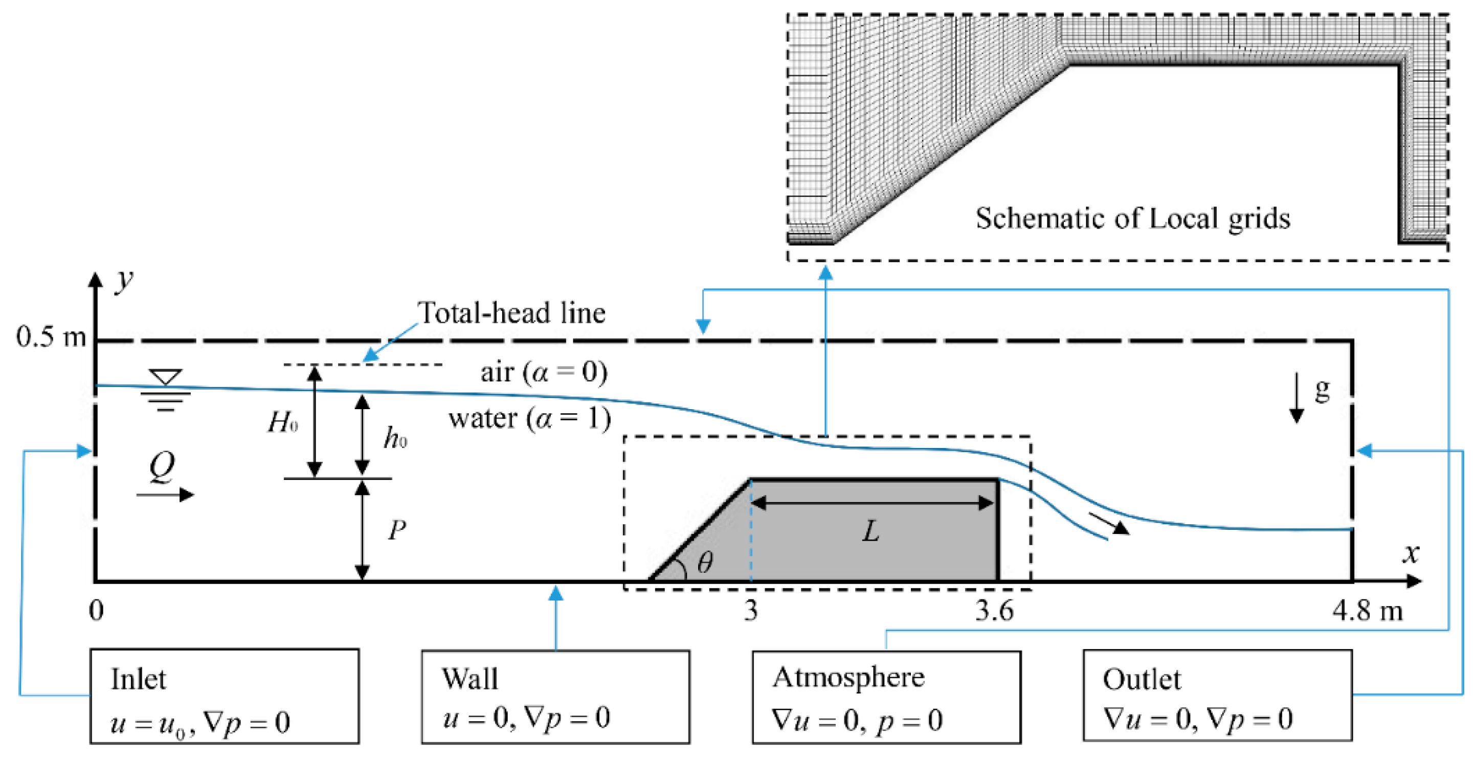
Numerical simulations were employed to investigate the flow characteristics based on the physical experiments of Goodarzi, Farhoudi et al. [33], which were conducted in a horizontal rectangular flume that was 12 m long, 0.25 m wide, and 0.50 m tall. The broad-crested weir had two parts in the longitudinal cross-section: an upstream face and a rectangular crest. A total of 40 tests, including eight different broad-crested weir configurations (with different upstream face angles θ = 10°, 15°, 22.5°, 30°, 45°, 60°, 75°, 90°) and five different discharge rates (Q = 0.015–0.035 m3/s) were conducted in their laboratory experiments. Both the height (P) and the width of the weir crest in the direction of flow (L) are 0.25 m. The geometry in the simulation domain was 4.8 m × 0.5 m (x × y) (see Figure 1). The distance from the inlet boundary to the weir exceeded 10 times the height of the weir to minimize the influence of the inlet boundary. All eight geometries have been investigated at a single discharge Q = 0.035 m3/s. The purpose of the study was to simulate the flow fields under free-flow conditions; therefore, the tail water level was kept low.
2.5. Boundary Conditions and Mesh
The boundary conditions (BCs) imposed on the numerical domain were at the flume inlet and outlet, at the free surface, and the walls (flume and weir). To match the experimental conditions, a variableHeightFlowRateInletVelocity boundary was applied to U at the inlet boundary, which adjusted the flow depth and velocity at the inlet to obtain a constant flow rate (Q) and a variableHeightFlowRate boundary condition was used to enable the water level to oscillate [21]. The outlet boundary was controlled by a zero gradient (Neuman BC) velocity condition, and no-slip boundary conditions were imposed on all walls. The top surface of the mesh was considered a free surface, and a pressureInletOutletVelocity condition for U was imposed to allow the flow to enter and leave the simulation domain freely [26]. Regarding the variables in the RANS model, the values of k, ε, and ω at the inlet and outlet boundaries were set to arbitrary low values and allowed to develop within the simulation domain [29]. The standard wall function was employed so that the governing equations could be solved correctly. A detailed explanation of the BCs can be found in Moukalled, Mangani et al. [34]. Structured and uniform mesh systems were used for the entire computational domain. In the near-wall region, ten boundary layers contracting with a ratio of 1.2 were placed at the flume and bottom walls to ensure that y+ remained within the viscous sublayer.
3. Results
3.1. Discretization Error Analysis
Mesh sensitivity was tested using the grid convergence index (GCI) method, which is a widely accepted and recommended method for estimating discretization error that has been applied to several hundred CFD cases [35]. The GCI is a measure of how far the simulation result is from the asymptotic numerical result. A small GCI means the simulation is within the asymptotic range [36].
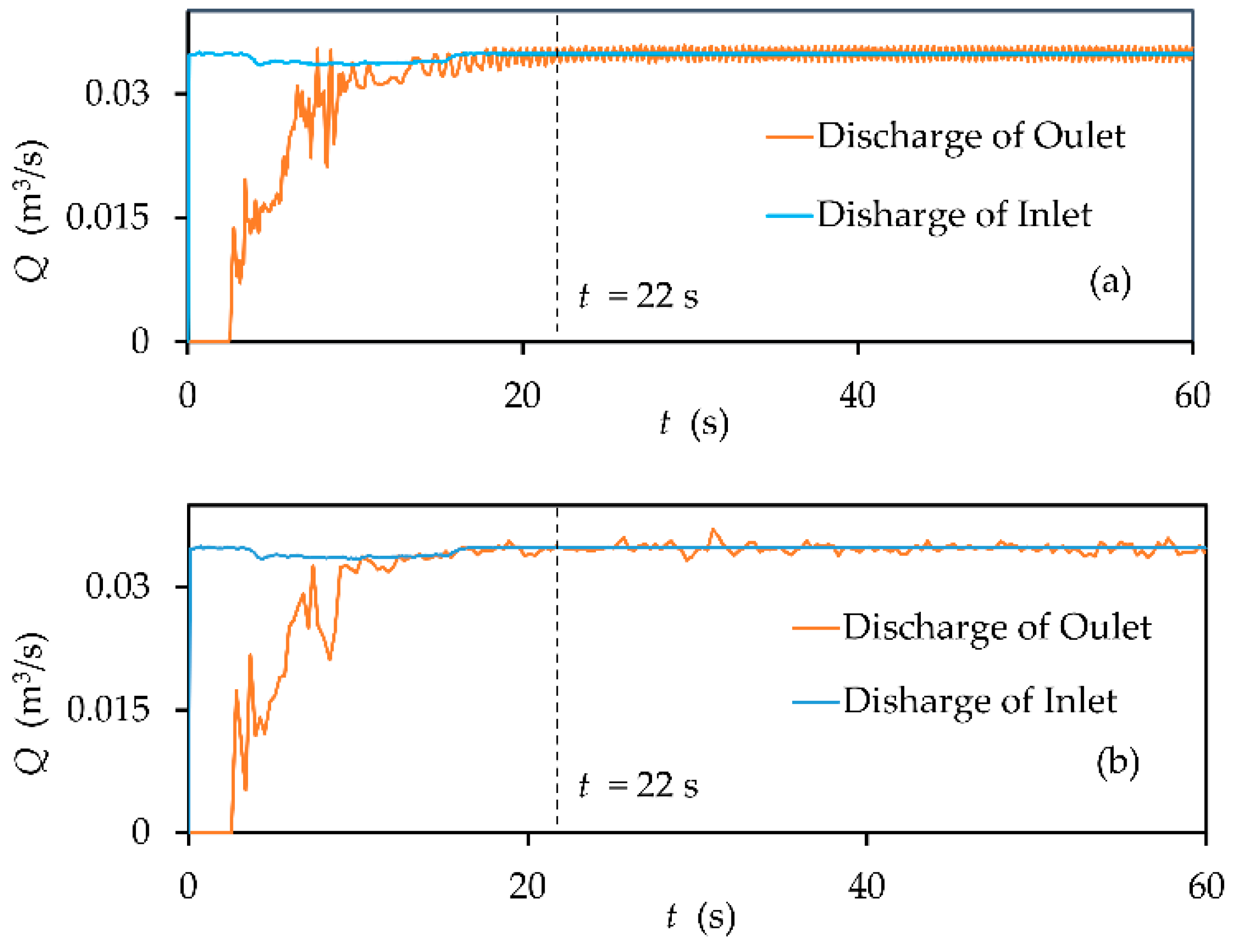
Because performing uncertainty analyses of all 16 simulations is a very time-consuming task, only three broad-crested weir configurations (θ = 30°, 45°, and 90°) with Q = 0.035 m3/s was analyzed; these were assumed to represent all the simulations in this study. The water depth (h1) was selected in three different sections to compute the GCI; these sections were labeled section A-A x = 3.0 m, section B-B x = 3.3 m, and section C-C x = 3.6 m. Three different mesh resolutions, N1 = 158,556, N2 = 114,640, and N3 = 81,872 (fine mesh, medium mesh, and coarse mesh) were employed for this study. Before the discretization error was estimated, the simulation’s convergence was evaluated based on the mass balance of the water phase between the inflow and outflow boundaries. Based on the calculation results for each simulation, when the calculation time t > 22 s, the flow discharges of inlet and outlet tend to be consistent. Therefore, a total calculation time T = 60 s can ensure that each simulation is convergent. Figure 2 presents the convergence history of low discharge for θ = 30°.
After convergence had been reached, the GCI was calculated using the following equation:
where e is the error between two adjacent meshes, and , where fi (i = 1, 2, 3) is the value of the indicator variable f (the water depth). Fs is a safety factor. Fs = 1.25 for comparison of three or more meshes. r is the mesh refinement ratio ( and ). p is the local order of accuracy. In this study, the average order of accuracy (pave) was used to calculate the GCI.
Table 1 presents the calculated GCIs for the three meshes. In Table 1, the values of GCI12 and GCI23 represent the relative change from medium to fine mesh and from coarse to medium mesh, respectively. According to this table, the maximum numerical uncertainty in the discretization using the computed water depths for Mesh 1 and Mesh 2 are 0.511% and 1.360%, respectively; these correspond to water depths of ±0.398 mm and ±1.068 mm, respectively. Besides, values of approaching 1 indicate that the simulation results are in the asymptotic range. In general, the use of the medium mesh of 114,640 cells is sufficient for the present investigation.
3.2. Free-Surface Profiles
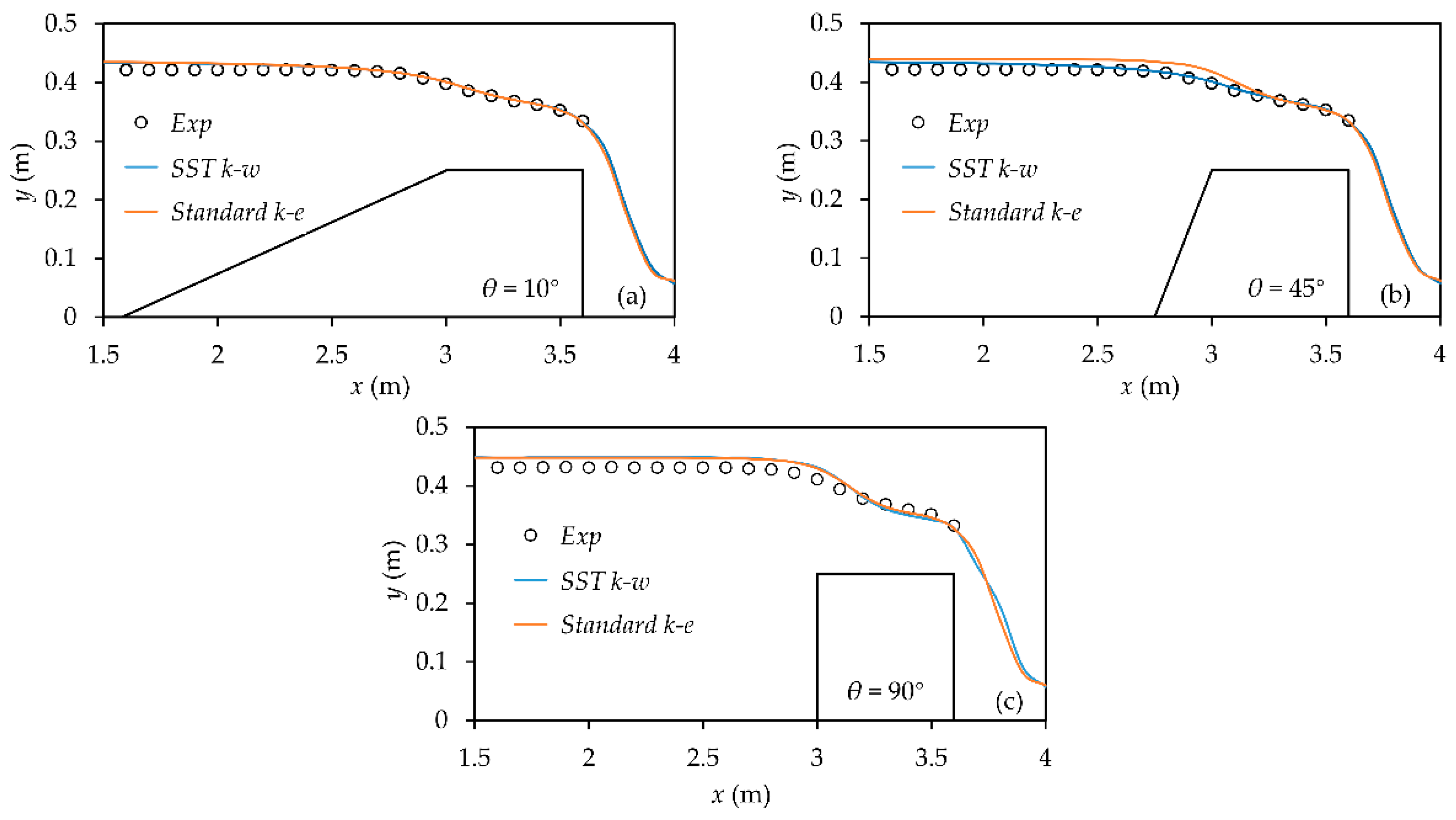
Discharge over the broad-crested weir in this study is 0.035 m3/s. Figure 3 compares numerical and experimental free-surface profiles for three typical broad-crested weir configurations (θ = 10°, 45° and 90°). Chen et al. [37] divide the free-surface profile into two parts based on the gradient: a slowly descending part and a sharply descending part. The curvature of the former part is close to zero, whereas that of the latter part decreases quickly with a hydraulic drop. As shown in Figure 3, the free-surface profiles in this study are consistent with their conclusion. To further verify the reliability of the numerical simulation, two statistical indicators, the root mean square error (RMSE) and the mean absolute percent error (MAPE) are used to evaluate the accuracy of the numerical results (see Appendix A). Both the RMSE and the MAPE must be small to ensure a good agreement between the numerical and laboratory results. The calculated values of the statistical indicators for the free-surface profiles are listed in Table 2. As can be seen from Table 2, for the standard k-ε model, the value of RMSE is between 0.35% and 0.67%, and the value of MAPE is between 0.50% and 1.48%; for the SST k-w model, the value of RMSE is between 0.25% and 0.66%, and the value of MAPE is between 0.55% and 1.41%. Statistical results show that both turbulence models show good agreement in terms of predicting the free-surface profile over the broad-crested weir.
3.3. Discharge Coefficient
One of the objectives of this research is to study the effect of the upstream face angle on the discharge capacity of a broad-crested weir. The discharge coefficient of a broad-crested weir under the free-flow condition was defined by Hager [2] (see Equation (1)). Equation (1) has been widely used to calculate the discharge coefficient of broad-crested weirs under free-flow conditions. Table 3 shows the measured and computed discharge coefficients obtained by the standard k-ε model and the SST k-w model. In Table 3, REk-ε and REk-w are the relative errors for standard k-ε model and the SST k-w model, respectively. From Table 3, one may conclude the following:
- For the standard k-ε model and the SST k-w model, the maximum relative errors are 3.957% and 3.439%, respectively, which is an excellent indication.
- For 45° < θ ≤ 90°, the upstream angle increases Cd significantly. However, when θ is less than 45°, the effect of the upstream angle on Cd is no longer obvious. In other words, an upstream slope of less than 45° is more expensive in construction terms and does not improve Cd. Note that this value of θ is approximately 60° (1V:0.5H), as recommended by Noori and Juma [39].
In general, an increasing upstream angle θ has a negative effect on the discharge coefficient Cd.
3.4. Computed Streamline Patterns
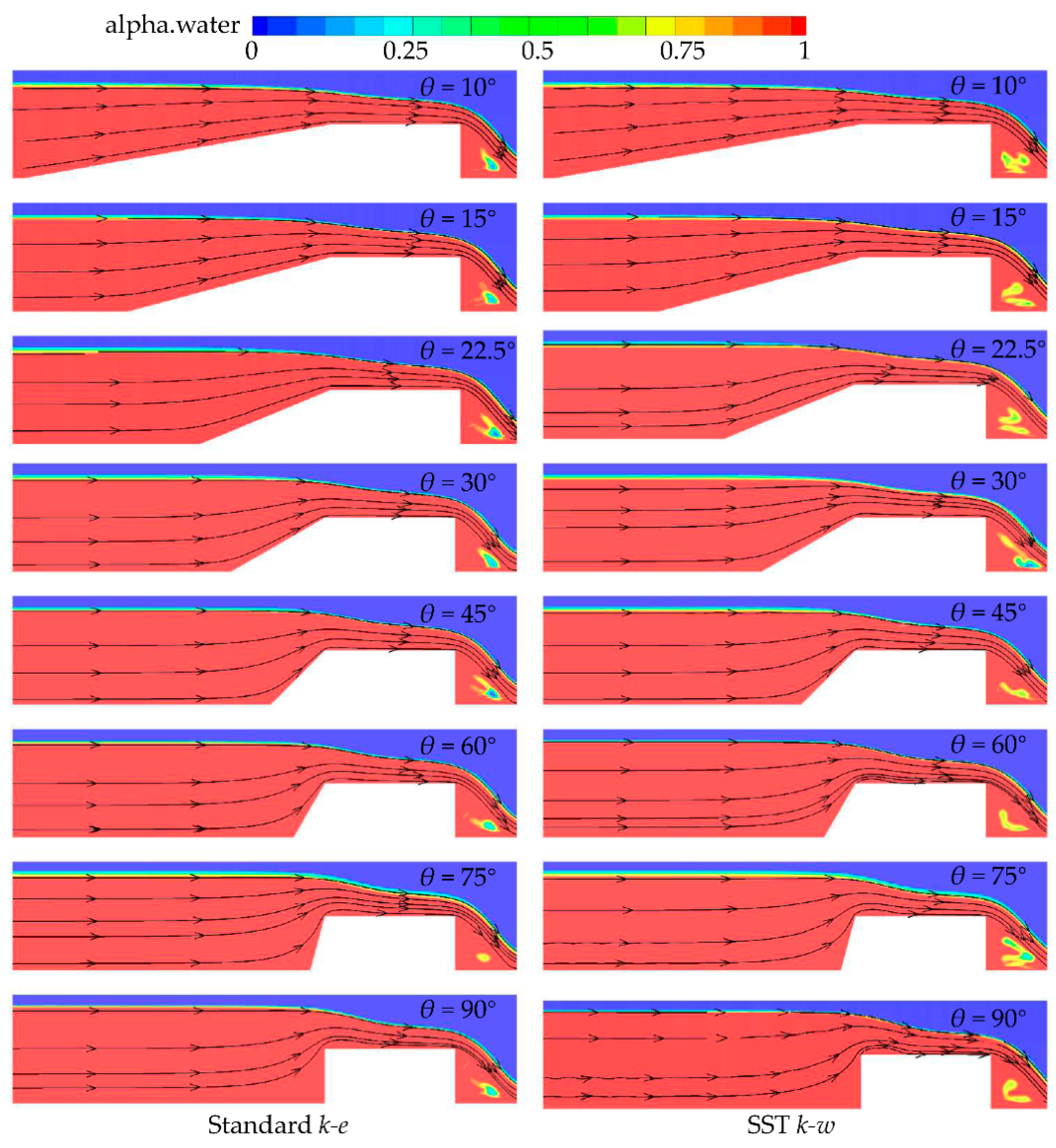
The computed streamline patterns for all configurations with Q = 0.035 m3/s are shown in Figure 4. Figure 4 shows that the upstream face angle θ has an obvious effect on the flow pattern. For 10° ≤ θ ≤ 30°, the streamlines are almost parallel, indicating that the flow characteristics are good, and the hydraulic loss is small. As θ increases, streamlines become less parallel. For 60° ≤ θ ≤ 90°, a flow separation region can be found on the rectangular crest; this is called the crest recirculation zone [40]. The separation region influences the discharge performance of a weir [2,38,40,41]. In short, Figure 4 shows a strong effect of the upstream angle on the flow field structure of the broad-crested weir in the streamline patterns; and the flow fields obtained by the two turbulence models are basically similar.
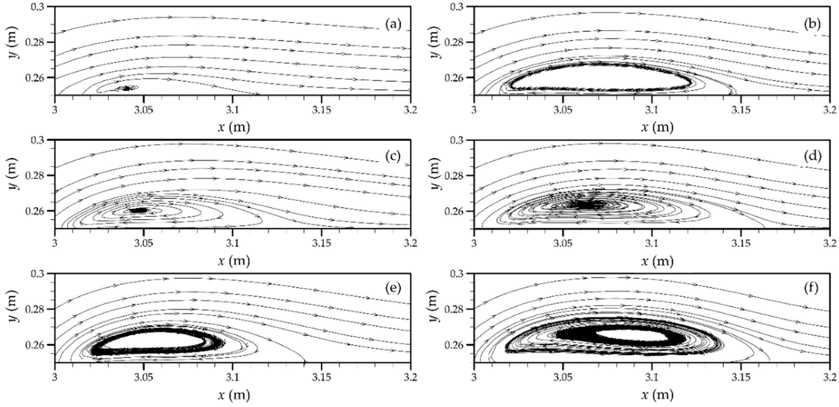
Many researchers have shown that the crest separation zone has a major influence on the discharge coefficient [2,10]. To further understand the impact of the upstream angle on flow separation zone, the shape of the crest separation zone for θ = 60°, θ = 75°, and θ = 90° with Q = 0.035 m3/s are given in Figure 5. The present results show that both the standard k-e model and the standard k-w model can capture the crest separation zone; the area of separation zone predicted by the standard k-e model is smaller than the prediction result of the SST k-w model. Notably, it was impossible to capture the flow separation for θ <60° with the medium mesh used in this study because this separation is quite small, according to the measured data of Madadi et al. [38]. As θ increases, the area of this zone will increase. Combined with the calculated discharge coefficient, the flow separation zone has a negative effect on a broad-crested weir’s discharge coefficient [33]. Referring to Zachoval et al. [42], shape of separation zone is difficult to determine because the separation zone depends on time and the Reynolds number (inflow condition); therefore, numerical methods provide an effective complement to experiments when studying such issues.
4. Conclusions
In these simulations, flow discharge Q = 0.035 m3/s and upstream face angles from θ = 10° to 90° were considered. The influence of the upstream slope face on a trapezoidal broad-crested weir was investigated using OpenFOAM. Discretization error analyses using a GCI were performed for three mesh resolutions. Two turbulence models—the standard k-e model and the SST k-w model—were used in this study. The numerical results indicate that the InterFoam solver of OpenFOAM can provide a good prediction of the free-surface profile and discharge coefficient. For trapezoidal broad-crested weirs, the upstream angle θ has a negative impact on the discharge coefficient Cd. For a certain flow discharge rate, Cd increases as θ decreases. Additionally, a crest separation zone is observed when θ ≥ 60°. As θ increases, the area of the separation zone increases. The area of separation zone predicted by the standard k-e model is smaller than the prediction result of the SST k-w model.
Author Contributions
This paper is done under the joint effort of all authors. Conceptualization, L.J. and M.D.; Methodology, L.J.; Software, L.J.; Validation, L.J., M.D. and Y.R.; Formal Analysis, L.J.; Investigation, H.S.; Resources, Y.R.; Data Curation, H.S.; Writing—Original Draft Preparation, L.J.; Writing—Review & Editing, L.J. and M.D.; Visualization, H.S.; Supervision, M.D.
Funding
This research received no external funding.
Conflicts of Interest
The authors declare no conflicts of interest.
Nomenclature
The following symbols are used in this study:
| b | width of weir (in the direction perpendicular to the flow direction); |
| Cd | discharge coefficient; |
| e | error between two adjacent meshes; |
| Fs | safety factor; |
| gravity force; | |
| f | value of indicator variable; |
| g | gravitational acceleration; |
| GCI | grid convergence index; |
| H0 | upstream total head; |
| h0 | upstream overflow piezometric head; |
| L | width of weir crest in the flow direction; |
| MAPE | mean absolute percent error; |
| P | weir height; |
| time-averaged pressure; | |
| p | local order of accuracy; |
| Q | flow discharge rate; |
| q | unit discharge; |
| Re | Reynolds number; |
| RE | relative error; |
| R2 | determination coefficient. |
| r | mesh refinement ratio; |
| RMSE | root mean square error; |
| T | total simulation time. |
| t | time; |
| time-averaged velocity vector; | |
| W | Weber number; |
| y+ | dimensionless wall distance; |
| α | volume fraction; |
| θ | upstream face angle; |
| λ | generic fluid property; |
| μ | viscosity of water; |
| ξ | relative crest length; |
| ρ | density; |
| σ | surface tension of water. |
Appendix
Root mean square error (RMSE):
Mean absolute percent error (MAPE):
Coefficient of determination (R2):
Relative error (RE):
where yO and yP are the experimental results and numerical results (or predicted results), respectively. N is the number of samples.
References
- Felder, S.; Islam, N. Hydraulic Performance of an Embankment Weir with Rough Crest. J. Hydraul. Eng. 2017, 143, 04016086. [Google Scholar] [CrossRef]
- Hager, W.H.; Schwalt, M. Broad-crested weir. J. Irrig. Drain. Eng. 1994, 120, 13–26. [Google Scholar] [CrossRef]
- Tracy, H.J. Discharge Characteristics of Broad-Crested Weirs; US Department of the Interior, Geological Survey: Washington, DC, USA, 1957.
- Isaacs, L.T. Effects of Laminar Boundary Layer on a Model Broad-Crested Weir; University of Queensland: Brisbane, Australia, 1981. [Google Scholar]
- Horton, R.E.; Murphy, E.C. Weir Experiments, Coefficients, and Formulas; US Government Printing Office: Washington, DC, USA, 1906.
- Kindsvater, C.E. Discharge Characteristics of Embankment-Shaped Weirs; US Government Printing Office: Washington, DC, USA, 1964.
- Fritz, H.M.; Hager, W.H. Hydraulics of embankment weirs. J. Hydraul. Eng. 1998, 124, 963–971. [Google Scholar] [CrossRef]
- Sargison, J.E.; Percy, A. Hydraulics of broad-crested weirs with varying side slopes. J. Irrig. Drain. Eng. 2009, 135, 115–118. [Google Scholar] [CrossRef]
- Azimi, A.H.; Rajaratnam, N.; Zhu, D.Z. Discharge Characteristics of Weirs of Finite Crest Length with Upstream and Downstream Ramps. J. Irrig. Drain. Eng. 2013, 139, 75–83. [Google Scholar] [CrossRef]
- Madadi, M.R.; Dalir, A.H.; Farsadizadeh, D. Control of undular weir flow by changing of weir geometry. Flow Meas. Instrum. 2013, 34, 160–167. [Google Scholar] [CrossRef]
- Hakim, S.S.; Azimi, A.H. Hydraulics of Submerged Triangular Weirs and Weirs of Finite-Crest Length with Upstream and Downstream Ramps. J. Irrig. Drain. Eng. 2017, 143, 06017008. [Google Scholar] [CrossRef]
- Sarker, M.A.; Rhodes, D.G. Calculation of free-surface profile over a rectangular broad-crested weir. Flow Meas. Instrum. 2004, 15, 215–219. [Google Scholar] [CrossRef]
- Kirkgoz, M.S.; Akoz, M.S.; Oner, A.A. Experimental and theoretical analyses of two-dimensional flows upstream of broad-crested weirs. Can. J. Civ. Eng. 2008, 35, 975–986. [Google Scholar] [CrossRef]
- Haun, S.; Olsen, N.R.B.; Feurich, R. Numerical Modeling of Flow Over Trapezoidal Broad-Crested Weir. Eng. Appl. Comput. Fluid Mech. 2011, 5, 397–405. [Google Scholar] [CrossRef] [Green Version]
- Akoz, M.S.; Gumus, V.; Kirkgoz, M.S. Numerical Simulation of Flow over a Semicylinder Weir. J. Irrig. Drain. Eng. 2014, 140, 04014016. [Google Scholar] [CrossRef]
- Lobosco, R.; Schulz, H.; Simões, A. Analysis of two phase flows on stepped spillways. In Hydrodynamics-Optimizing Methods and Tools; InTech: London, UK, 2011. [Google Scholar]
- Sweeney, B.P. Converged Stepped Spillway Models in OpenFOAM. Master’s Thesis, Kansas State University, Manhattan, KS, USA, 2014. [Google Scholar]
- Duguay, J.M.; Lacey, R.W.J.; Gaucher, J. A case study of a pool and weir fishway modeled with OpenFOAM and FLOW-3D. Ecol. Eng. 2017, 103, 31–42. [Google Scholar] [CrossRef]
- Kızılaslan, M.A.; Demirel, E. Numerical Investigation of the Recirculation Zone Length Upstream of the Round-Nosed Broad Crested Weir. In Proceedings of the International Conference on Urban Design, Transportation, Architectural and Environmental Engineering, Istanbul, Turkey, 8–10 September 2017. [Google Scholar]
- Toro, J.P.; Bombardelli, F.A.; Paik, J. Detached Eddy Simulation of the Nonaerated Skimming Flow over a Stepped Spillway. J. Hydraul. Eng. 2017, 143, 04017032. [Google Scholar] [CrossRef]
- Fuentes-Pérez, J.F.; Silva, A.T.; Tuhtan, J.A.; García-Vega, A.; Carbonell-Baeza, R.; Musall, M.; Kruusmaa, M. 3D modelling of non-uniform and turbulent flow in vertical slot fishways. Environ. Model. Softw. 2018, 99, 156–169. [Google Scholar] [CrossRef]
- Launder, B.E.; Sharma, B.I. Application of the energy-dissipation model of turbulence to the calculation of flow near a spinning disc. Lett. Heat Mass Transf. 1974, 1, 131–137. [Google Scholar] [CrossRef]
- Wilcox, D.C. Reassessment of the scale-determining equation for advanced turbulence models. AIAA J. 1988, 26, 1299–1310. [Google Scholar] [CrossRef]
- Menter, F.; Esch, T. Elements of industrial heat transfer predictions. In Proceedings of the 16th Brazilian Congress of Mechanical Engineering (COBEM), Uberlândia, Brazil, 26–30 November 2001. [Google Scholar]
- Menter, F.R.; Kuntz, M.; Langtry, R. Ten years of industrial experience with the SST turbulence model. Turbul. Heat Mass Transf. 2003, 4, 625–632. [Google Scholar]
- Bayon, A.; Toro, J.P.; Bombardelli, F.A.; Matos, J.; López-Jiménez, P.A. Influence of VOF technique, turbulence model and discretization scheme on the numerical simulation of the non-aerated, skimming flow in stepped spillways. J. Hydro-Environ. Res. 2018, 19, 137–149. [Google Scholar] [CrossRef]
- Beg, M.N.A.; Carvalho, R.F.; Tait, S.; Brevis, W.; Rubinato, M.; Schellart, A.; Leandro, J. A comparative study of manhole hydraulics using stereoscopic PIV and different RANS models. Water Sci. Technol. 2018. [Google Scholar] [CrossRef] [PubMed]
- Hirt, C.W.; Nichols, B.D. Volume of fluid (VOF) method for the dynamics of free boundaries. J. Comput. Phys. 1981, 39, 201–225. [Google Scholar] [CrossRef]
- Bayon, A.; Valero, D. Performance assessment of OpenFOAM and FLOW-3D in the numerical modeling of a low Reynolds number hydraulic jump. Environ. Model. Softw. 2016, 80, 322–335. [Google Scholar] [CrossRef]
- Bayon-Barrachina, A. Numerical analysis of hydraulic jumps using OpenFOAM. J. Hydroinform. 2015, 17, 662–678. [Google Scholar] [CrossRef] [Green Version]
- OpenFOAM User Guide; OpenFOAM Foundation: London, UK, 2011; Available online: https://www.openfoam.com/documentation/user-guide/ (accessed on 14 November 2018).
- Zhou, Z.; Hsu, T.J.; Cox, D.; Liu, X. Large-eddy simulation of wave-breaking induced turbulent coherent structures and suspended sediment transport on a barred beach. J. Geophys. Res. 2017, 122, 207–235. [Google Scholar] [CrossRef]
- Goodarzi, E.; Farhoudi, J.; Shokri, N. Flow Characteristics of Rectangular Broad-Crested Weirs with Sloped Upstream Face. J. Hydrol. Hydromech. 2012, 60, 87–100. [Google Scholar] [CrossRef]
- Moukalled, F.; Mangani, L.; Darwish, M. Boundary Conditions in OpenFOAM® and uFVM; Springer International Publishing: Berlin/Heidelberg, Germany, 2016; pp. 745–759. [Google Scholar]
- Jak, E.; Hayes, P.C. Procedure of Estimation and Reporting of Uncertainty Due to Discretization in CFD Applications. J. Fluids Eng. 2008, 130, 078001. [Google Scholar]
- Elsayed, K.; Lacor, C. CFD modeling and multi-objective optimization of cyclone geometry using desirability function, artificial neural networks and genetic algorithms. Appl. Math. Model. 2013, 37, 5680–5704. [Google Scholar] [CrossRef]
- Chen, Y.; Fu, Z.; Chen, Q.; Cui, Z. Discharge Coefficient of Rectangular Short-Crested Weir with Varying Slope Coefficients. Water 2018, 10, 204. [Google Scholar] [CrossRef]
- Madadi, M.R.; Dalir, A.H.; Farsadizadeh, D. Investigation of flow characteristics above trapezoidal broad-crested weirs. Flow Meas. Instrum. 2014, 38, 139–148. [Google Scholar] [CrossRef]
- Noori, B.M.A.; Juma, I.A.K. Performance Improvement of Broad Crested Weirs. AL Rafdain Eng. J. 2009, 17, 95–107. [Google Scholar]
- Zachoval, Z.; Roušar, L. Flow structure in front of the broad-crested weir. In Proceedings of the Experimental Fluid Mechanics 2014, Český Krumlov, Czech Republic, 18–21 November 2014; p. 02117. [Google Scholar]
- Hargreaves, D.; Morvan, H.; Wright, N. Validation of the volume of fluid method for free surface calculation: The broad-crested weir. Eng. Appl. Comput. Fluid Mech. 2007, 1, 136–146. [Google Scholar] [CrossRef]
- Zachoval, Z.; Mistrová, I.; Roušar, L.; Šulc, J.; Zubík, P. Zone of flow separation at the upstream edge of a rectangular broad-crested weir/Oblast odtržení proudu na návodní hraně pravoúhlého přelivu se širokou korunou. J. Hydrol. Hydromech. 2012, 60, 288–298. [Google Scholar] [CrossRef]
Figure 1.
General scheme of the broad-crested weir.

Figure 2.
Convergence history of computational fluid dynamics (CFD) flow discharge for θ = 30° (Q = 0.035 m3/s): (a) the standard k-ε model; and (b) the SST k-w model.
Figure 2.
Convergence history of computational fluid dynamics (CFD) flow discharge for θ = 30° (Q = 0.035 m3/s): (a) the standard k-ε model; and (b) the SST k-w model.

Figure 3.
Free-surface profiles (Q = 0.035 m3/s): (a) θ = 10°; (b) θ = 45°; (c) θ = 90°.

Figure 4.
Computed streamline patterns (Q = 0.035 m3/s).

Figure 5.
Crest separation zones (Q = 0.035 m3/s): (a) θ = 60°, standard k-e; (b) θ = 60°, SST k-w; (c) θ = 75°, standard k-e; (d) θ = 75°, SST k-w; (e) θ = 90°, standard k-e; and (f) θ = 90°, SST k-w.
Figure 5.
Crest separation zones (Q = 0.035 m3/s): (a) θ = 60°, standard k-e; (b) θ = 60°, SST k-w; (c) θ = 75°, standard k-e; (d) θ = 75°, SST k-w; (e) θ = 90°, standard k-e; and (f) θ = 90°, SST k-w.


Table 1.
Grid convergence calculations using the grid convergence index (GCI) method.
| Angles | Turbulence Model | Section | h1 (m) | pave | GCI12 (%) | GCI23 (%) | GCI32/rpGCI21 | ||
|---|---|---|---|---|---|---|---|---|---|
| f1 | f2 | f3 | |||||||
| θ = 30° | Standard k-e | A-A | 0.16288 | 0.16175 | 0.15969 | 2.138 | 0.025 | 0.023 | 0.8861 |
| B-B | 0.12100 | 0.12074 | 0.12014 | 2.138 | 0.008 | 0.018 | 1.0022 | ||
| C-C | 0.08010 | 0.08016 | 0.08022 | 2.138 | 0.003 | 0.003 | 0.9993 | ||
| SST k-w | A-A | 0.15784 | 0.15837 | 0.15464 | 8.240 | 0.193 | 1.352 | 0.9967 | |
| B-B | 0.11756 | 0.11843 | 0.11990 | 8.240 | 0.425 | 0.712 | 0.9927 | ||
| C-C | 0.08077 | 0.08107 | 0.08188 | 8.240 | 0.213 | 0.573 | 0.9963 | ||
| θ = 45° | Standard k-e | A-A | 0.16718 | 0.16772 | 0.16534 | 12.234 | 0.088 | 0.388 | 0.9968 |
| B-B | 0.12012 | 0.12008 | 0.12145 | 12.234 | 0.009 | 0.312 | 1.0003 | ||
| C-C | 0.08238 | 0.08224 | 0.08208 | 12.234 | 0.047 | 0.053 | 1.0017 | ||
| SST k-w | A-A | 0.16831 | 0.16832 | 0.15086 | 28.472 | 0.000 | 0.243 | 0.9999 | |
| B-B | 0.11759 | 0.11753 | 0.11987 | 28.472 | 0.001 | 0.047 | 1.0005 | ||
| C-C | 0.08170 | 0.07994 | 0.08409 | 28.472 | 0.050 | 0.122 | 1.0220 | ||
| θ = 90° | Standard k-e | A-A | 0.42985 | 0.42951 | 0.43008 | 3.861 | 0.137 | 0.231 | 1.0008 |
| B-B | 0.11402 | 0.11423 | 0.11447 | 3.861 | 0.320 | 0.365 | 0.9982 | ||
| C-C | 0.07816 | 0.07793 | 0.07854 | 3.861 | 0.511 | 1.360 | 1.0160 | ||
| SST k-w | A-A | 0.43169 | 0.43149 | 0.43092 | 6.326 | 0.041 | 0.116 | 1.0005 | |
| B-B | 0.11059 | 0.11033 | 0.11137 | 6.326 | 0.206 | 0.824 | 1.0024 | ||
| C-C | 0.07740 | 0.07709 | 0.07748 | 6.326 | 0.350 | 0.442 | 1.0040 | ||
Table 2.
Root mean square error (RMSE) and mean absolute percent error (MAPE) (%) for the numerical results of free-surface profiles.
Table 2.
Root mean square error (RMSE) and mean absolute percent error (MAPE) (%) for the numerical results of free-surface profiles.
| Model | θ = 10° | θ = 45° | θ = 90° | |||
|---|---|---|---|---|---|---|
| RMSE | MAPE | RMSE | MAPE | RMSE | MAPE | |
| Standard k-e | 0.35 | 0.50 | 0.67 | 1.48 | 0.58 | 0.67 |
| SST k-w | 0.25 | 0.55 | 0.66 | 1.41 | 0.44 | 0.76 |
Table 3.
Comparisons of measured and computed coefficient from CFD.
| θ | Exp | Cdk-e | Cdk-w | REk-e (%) | REk-w (%) |
|---|---|---|---|---|---|
| 10° | 0.412 | 0.406 | 0.402 | 1.458 | 2.394 |
| 15° | 0.404 | 0.389 | 0.390 | 3.656 | 3.439 |
| 22.5° | 0.396 | 0.380 | 0.386 | 3.957 | 2.327 |
| 30° | 0.385 | 0.378 | 0.380 | 1.656 | 1.357 |
| 45° | 0.383 | 0.369 | 0.370 | 3.451 | 3.261 |
| 60° | 0.368 | 0.367 | 0.355 | 0.256 | 3.458 |
| 75° | 0.355 | 0.353 | 0.353 | 0.440 | 0.440 |
| 90° | 0.347 | 0.345 | 0.344 | 0.532 | 0.990 |
© 2018 by the authors. Licensee MDPI, Basel, Switzerland. This article is an open access article distributed under the terms and conditions of the Creative Commons Attribution (CC BY) license (http://creativecommons.org/licenses/by/4.0/).
Share and Cite
MDPI and ACS Style
Jiang, L.; Diao, M.; Sun, H.; Ren, Y. Numerical Modeling of Flow Over a Rectangular Broad-Crested Weir with a Sloped Upstream Face. Water 2018, 10, 1663. https://doi.org/10.3390/w10111663
AMA Style
Jiang L, Diao M, Sun H, Ren Y. Numerical Modeling of Flow Over a Rectangular Broad-Crested Weir with a Sloped Upstream Face. Water. 2018; 10(11):1663. https://doi.org/10.3390/w10111663
Chicago/Turabian StyleJiang, Lei, Mingjun Diao, Haomiao Sun, and Yu Ren. 2018. "Numerical Modeling of Flow Over a Rectangular Broad-Crested Weir with a Sloped Upstream Face" Water 10, no. 11: 1663. https://doi.org/10.3390/w10111663
Note that from the first issue of 2016, this journal uses article numbers instead of page numbers. See further details here.