Article

Physical and Biological Water Column Observations during Summer Sea/Land Breeze Winds in the Coastal Northern Tyrrhenian Sea

by
Riccardo Martellucci
*,
Alberto Pierattini
,
Francesco Paladini De Mendoza
,
Cristiano Melchiorri
,
Viviana Piermattei
and
Marco Marcelli
Laboratory of Experimental Oceanology and Marine Ecology, Department of Ecology and Biology, Tuscia University, 00053 Civitavecchia, Italy
*
Author to whom correspondence should be addressed.
Water 2018, 10(11), 1673; https://doi.org/10.3390/w10111673
Submission received: 31 August 2018 / Revised: 2 November 2018 / Accepted: 7 November 2018 / Published: 16 November 2018
(This article belongs to the Section Hydrology)

Abstract

:
Coupling between sea/land breeze and coastal circulation and the influence of wind-driven dynamics are substantially relevant for understanding coastal Mediterranean ecosystems. These coastal areas are particularly dynamic and are characterized by high-variable processes which drive biological phenomena at different time-scales. For the Tyrrhenian Sea, the available information on coastal dynamics is confined to large-scale general circulation with a focus exclusively on mesoscale pelagic dynamical processes. Hydrodynamic studies of Tyrrhenian coastal areas are very rare and focus on surface water circulation. For time scales that are associated with coastal water circulation, there is also limited knowledge on water column dynamics that are forced by local atmospheric circulations. This paper presents physical and biological data to document the effect of sea/land breeze circulation on ocean current dynamics and water column structures in a Northern Tyrrhenian coastal site. This coastal area is characterized by the presence of a relevant energy production site as well as one of the most important ports in the Mediterranean Sea for cruise traffic. Consequently, this coastal site is a transit point for many tourists and it is characterized by an increase of energy demand, especially during the summer season. The in-situ data show that coastal currents are predominantly controlled by the tide and local wind and respond rapidly to changes in wind direction. Water column thermal structure analyses reveal significant changes with the morning’s rotation of breeze: lifting of isotherms (cooling) was typically observed in deep layers during early mornings, accompanied by fluctuations in isotherms. The performed investigations provide valuable inputs for coastal ecosystem modeling and for a better understanding of the coastal processes that are significant for environmental and navigational interests.

1. Introduction

In the summer, coastal systems are often dominated by daily patterns of local breeze circulation. This holds true especially during periods of fair weather [1], when breeze circulation produces coastal dynamics that result in current and buoyancy-driven motions. During daytime, a gradient of horizontal pressure is established towards the land (sea breeze), while at night, this breeze reverses its course (land breeze) [2]. Sea breezes are generally more intense than land breezes. This difference occurs due to the land-sea thermal gradient, which is most evident when synoptic-scale winds are either weak [3] or strong [4].
The wind generally rotates clockwise during the day, moving offshore at night and onshore during the morning. Complex terrains have a strong influence on breeze circulation patterns [5] and can result in deviations of the breeze flow [6]. Non-uniform changes in the land/sea breeze direction occur over time due to the Coriolis Effect, pressure gradients from diurnal heating (cross-shore pressure gradient) and pressure gradients that are unaffected by diurnal changes [7]. This local atmospheric circulation significantly affects the dynamic processes operating on the coast at different temporal and spatial scales, resulting in highly variable phenomena [8]. Nearshore currents are coherent with the daily breeze cycle [9,10] responding rapidly (3–5 h) to the change in wind direction and varying within a specific time scale (24 h), which is a typical sub-mesoscale phenomenon. Coastal dynamics that are linked to breeze circulation influence the water [11], modifying the physical and biological parameters on short temporal and spatial scales of less than 24 h. Many observations have focused on the role of land/sea breeze events in coastal upwelling and downwelling [12]. Also, high-variability processes could occur, such as internal gravity waves [13,14], especially in a well-stratified water column. In addition, wide-ranging external forcing (such as tides) and coastal morphology influence these dynamics, further increasing the spatial and temporal variability of the coastal system [15]. Several studies conducted in shelf areas have highlighted the importance of tides in the coastal current dynamics. The tide produces currents that influence the cross-shore transport and the internal motions. Pineda proposed that the internal tide produces an upwelling phenomenon, resulting in an advection of cold and dense water from the sub-surface layer [16].
Many authors have demonstrated a strong link between physical and biological dynamics [17], and such features have been observed in tides [18], wind-driven upwelling [19,20] and high frequency internal waves [21]. As phytoplankton production is strongly linked to physical forcing [22,23], which in coastal environments occurs at different time scales [24], the phytoplankton growth is synchronized with the associated dynamical processes, leading to increased primary production and biological trophic interactions [25]. Wind-driven processes play important roles in coastal ecosystems [26]. The induced current leads to pulses of nutrient input to the surface, nourishing primary producers, and transporting near-surface plankton over the shelves [27]. This influences the recruitment pulses of both intertidal invertebrates and commercially important fish species [28]. Furthermore, coastal zones are associated with an external input of nutrients, resulting in high nutrient levels, a condition under which physical forcing strongly affects coastal environments; with high nutrient levels, turbulence variations modify the characteristics of food web structures. In the absence of physical forcing, turbulence levels are low and dinoflagellates may, therefore, grow abnormally and result in harmful algal blooms [29].
Several studies [30,31,32] showed that the Tyrrhenian Sea is characterized by breeze circulation. Earlier work tended to be concerned with the role of the pollutant dispersion in the coastal zone [33,34,35]. However, hydrodynamic studies of the Tyrrhenian coastal zone are very limited [36,37] because the majority of literature focuses on general large-scale circulation, in particular on mesoscale pelagic dynamical processes [38,39,40,41]. The coastal zone of the herein investigated study area needs to receive an increasing amount of oceanographic attention both for the continuous port expansion and for a power plant that uses the coastal water as an engine cooling system. As already noted by Elliot [36] in 1981, “there is the basic requirement of a description of the currents and hydrographic properties of the shallow and coastal waters”, especially during the summer season that is characterized by an increase in cruise and tourist traffic as well as energy demand.
In this study, we collected oceanographic data by time series on a continental shelf with the support of current meter surveys in order to analyze the physical and biological processes on a daily scale, including the effects of breeze circulation on coastal currents, thermal patterns, and biomass in the water column. These results improve the knowledge about the time scales that are linked to sea breeze circulation and support the development of water quality models of the coastal zone.

2. Materials and Methods

The study area (Figure 1) is located in the Northern Tyrrhenian Sea along the coastal stretch between Mount Argentario and Capo Linaro [42,43]. The survey location is located off the coast of Civitavecchia, a port town that is located to the north of Rome. The mainland includes the Tolfa Mountains, which reach a maximum height of about 600 m. Marine terraces and cliffs dominate the coastal morphology, with small rocky and gravelly beaches [44]. The submerged morphology features a submerged beach that is characterized by steep slopes (>2°) down to ~40 m depth [45].
The atmospheric circulation strongly influences the dynamics in the Tyrrhenian basin [40,46] which is affected by mesoscale and seasonal variability [38,39,41].
Current records that were collected by Elliot and de Strobel in 1978 [36] showed significantly weak current near the Civitavecchia coast, with an average speed of less than 10 cm∙s−1 and presenting a 2 to 5 day variability. The surface currents also showed a significant amount of variability at the 2–3 day timescale. The mean alongshore flow at Civitavecchia was directed northwestwards along the coast and the mean speed measured 1 cm∙s−1 with a standard deviation of 3–5 cm∙s−1.
The wind in the study area shows two prevailing directions over the year, respectively from South/East (110° N–140° N) and North/Northeast (0° N–60° N) [47]. Compared to other seasons, during summer, the cross-shelf events increase, resulting in weak wind speeds of around 2 to 5 m∙s−1. Summer season climatology favors a high frequency of breeze events [30,31,32,48] due to the air-sea thermal gradient. This gradient produces a daily wind rotation, i.e., the wind moves offshore during the night and onshore during the day (Figure 2a).
Wind speed and sea surface temperature are strongly correlated to each other at their peak in a 24 h period, obeying daily cycles that are off phase by 5 h [48]. Statistical significance in coherence was calculated with the Goodman formula using the same methods as Thompson [49].

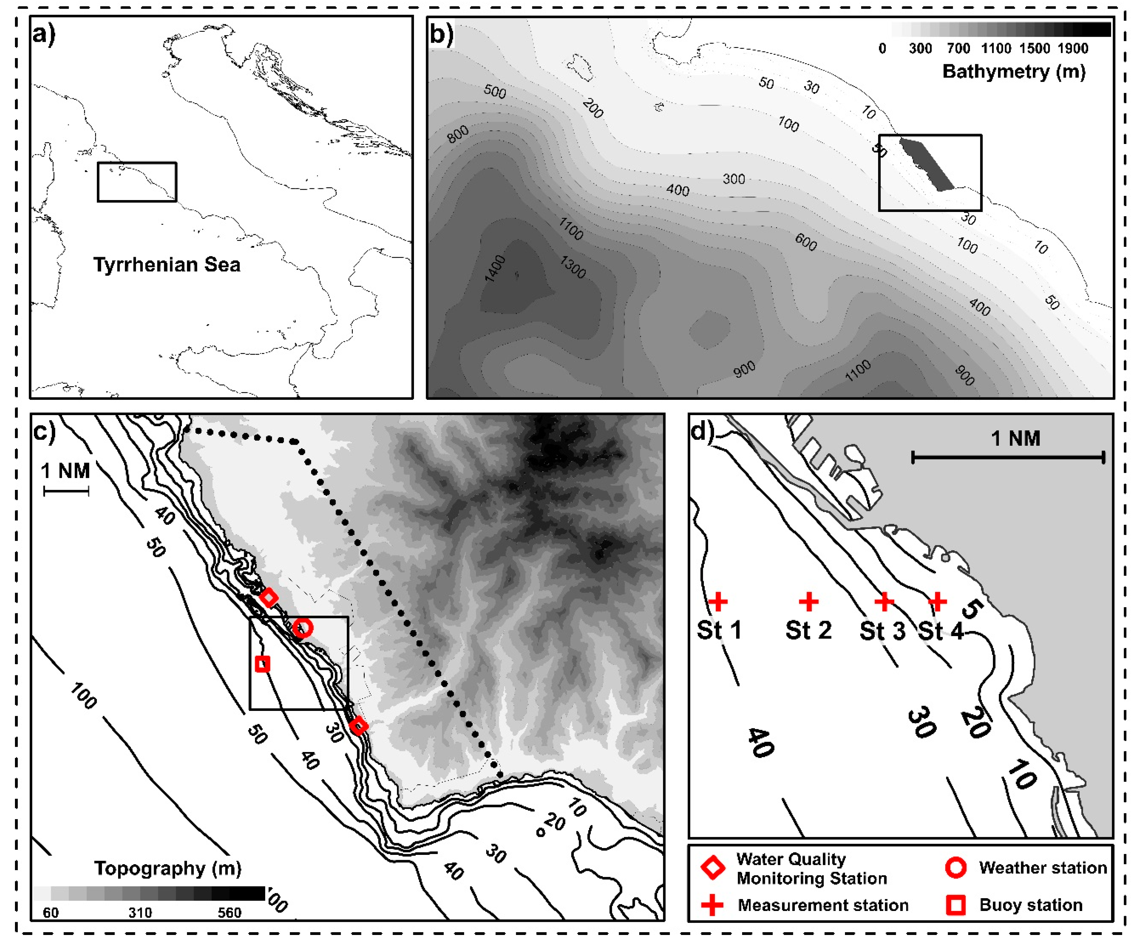
Sampling Survey Design

During the summers from 2012 to 2016, high-resolution observations were conducted in the study area. Data were collected at fixed stations [50] and hydrographical in situ surveys were performed using three different measuring strategies. The experiment aimed at identifying the variations of both the coastal circulation and the water column in response to the 180° rotation in the wind direction. During the surveys, current field, sea-water temperature, conductivity, and fluorescence of chlorophyll a (FChla) were acquired. Temperature, salinity, and chlorophyll a could be used to track coastal and ocean dynamics [51,52,53,54,55], which influence the motions of phytoplankton as a result of the interaction of current, buoyancy-driven motion and the convergent and divergent flows that are associated with internal waves and fronts [21].
During the summer of 2012 (Transect surveySupplementary Materials), the sampling plan (Figure 1, Figure 3a and Figure 4a) consisted of four evenly spaced stations (St. 1: ≈40 m; St. 2: ≈30 m; St. 3: ≈20 m; St. 4: ≈10 m), at which the time series were obtained with an interval of 20 min to study the FChla patch distribution in the coastal zone. During the same period, an oceanographic buoy that was placed near the stations acquired temperature, conductivity (salinity, density), and FChla on the sea-surface (1 m depth).
During the 2013–2015 survey (Fixed point surveySupplementary Materials), the time series were performed at a depth of 40 m at station St1. This station was chosen due to its low degree of seabed influence on the mixing phenomena compared to the other stations.
During the summer of 2016 (Gridded survey), the sampling plan (Figure 8d,e) consisted of 24 evenly distributed stations, where CTD (small instrument package) profiles were acquired.
The surveys were conducted between the end of August and the beginning of September (Table 1) since both cross-shelf events are more recurrent (Figure 2a) and the land/sea temperature gradient is more intense (Figure 2b) with respect to the other summer months.
All samplings were carried out from a small boat (5 m rigid inflatable) starting in the early morning (typically around 6:00) and lasted between 2 to 8 h depending on the weather conditions. During the surveys, in addition to yo-yo time series, current surveys were performed. Current data were collected by mean ADCP (Acoustic Doppler Current Profiler) SonTeck (500 kHz, sampling interval of 20 s to 60 s, average interval 50% sampling, cell thickness 1 m) which was deployed on the sea surface and was moored on the boat.
The time series was obtained using a small instrument package (CTD). The CTD contained an Idronaut 316 Plus multiparametric probe and a SeaPoint fluorometer. The sampling rate of the CTD was 10 Hz and was done by allowing the instrument package to fall freely at an average descent rate of 1 m∙s−1.

3. Results

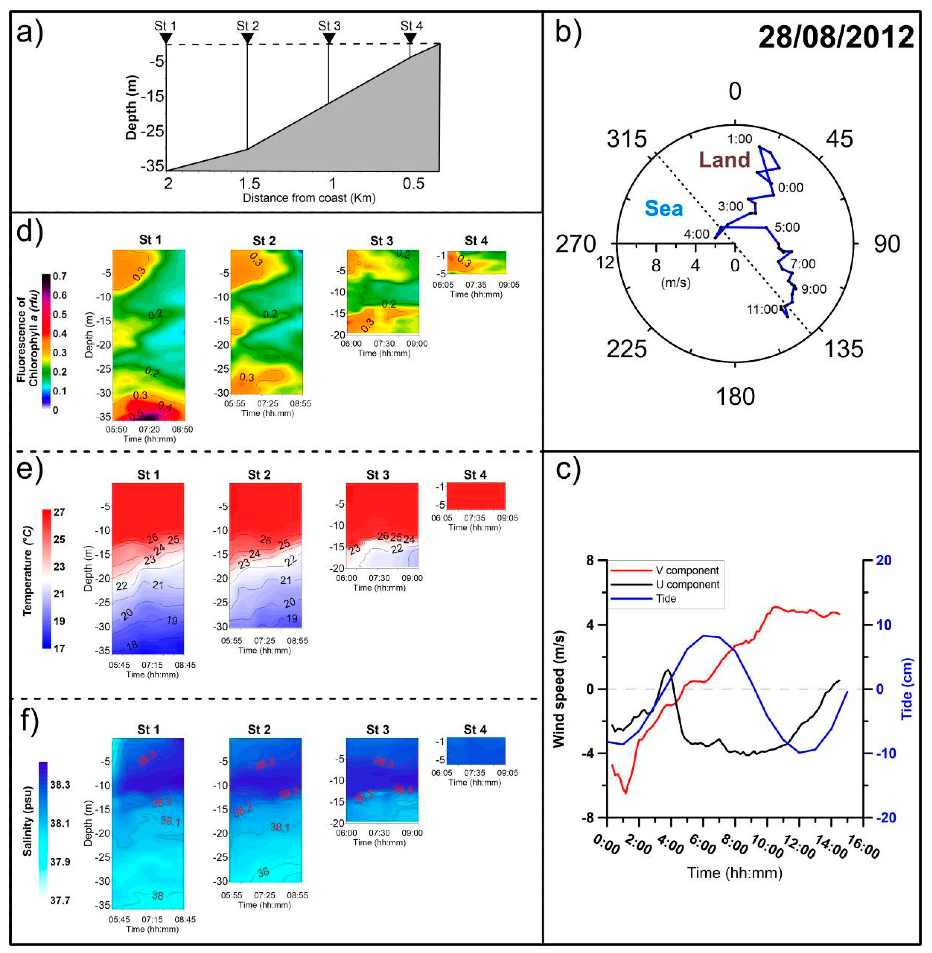
3.1. Transect Survey: Shows the Coast-Wide Gradient of the Fluorescence Patch and the Physical Characteristics of the Sea Water

During August 2012, FChla which was recorded by the oceanographic buoy showed a daily cycle (Figure 3a,b) that was characterized by a higher phase between 11:00 and 13:00 and a lower phase both in the early morning (between 4:00 and 6:00) and in the late afternoon (between 18:00 and 20:00). Spectral analysis of chlorophyll a highlights a peak at 24 h and a strong correlation between chlorophyll a and wind speed (Figure 3c).
During the surveys of 22 August 2012, the wind showed weak intensity and offshore direction during the night (Figure 4b,c). Land breeze blew for about seven hours, until 05:40 (starting at 22:20 on the previous day), turning progressively offshore from 5:30 and strengthening from 9:00. The wind Hodograph (Figure 4b) showed a clockwise rotation, typical of a breeze regime. The tide cycle (Figure 4c) had its minimum at 6:00 and raised to its maximum at 13:00 during which CTD measurements were performed.
At stations 1 and 2, a strong signal in FChla was detected (Figure 4d), which was subjected to an evident oscillation between 5 and 10 m depth that progressively diminished. A similar trend could be observed in the bottom layer exclusively at station 1, however to a lower extent than in the upper layer. Stations 3 and 4 do not show variability along the water column, however they show variations over time with a progressive decrease of fluorescence signal, especially in the surface layer. Concerning the water column thermal structure (Figure 4e), we measured a large thermal gradient at a 15 m depth of about 5 °C on the total gradient between the surface and bottom layer of 11 °C. During the survey, temperature increases in the surface layer, in the layer between 5 and 20 m depth oscillation occurs, and below 20 m depth temperature decreases. In stations 1 and 2, the 18 °C isotherms slope upward from the horizontal, sinking at about 5 m. This trend is evident in 17 °C isotherms only at station 2, while at station 1 it is parallel to the bottom. Along the water column, salinity (Figure 4f) generally shows a decrease of about 0.3 psu; over time, below 10 m depth, no changes emerge, while in the surface layer the salinity increases over time.
On 28 August 2012 the wind is offshore during the night, blowing for 9 h until 6:10, with a moderate intensity between 4 and 10 m∙s−1 (Figure 5b,c). The signal of FChla shows a decrease over time in the whole water column except for the bottom layer (Figure 5d). The decrease is more marked in the surface layer until 10 m depth. The gradient of FChla signal below 10 m depth is in agreement with the temperature trend which decreases by approximately 1 °C, whereas above 10 m depth, the water temperature is constant over time. The isotherms (Figure 5e) slope upward from the horizontal, especially in station 1 and 2. Station 3 presents a definite thermocline that is characterized by tight isotherms (roughly 23 °C to 26 °C). Above this layer, close to the bottom, the temperature decreases rapidly by about 2 °C. Concerning the salinity structure (Figure 5f) of station 1, the survey results show great variability in the surface layer (>10 m) where the salinity increases from 38.1 to 38.3 psu. The constantly largest salinity occurs between 5 and 15 m depth at stations 2 and 3 over time. Below 15 m, depth records show a uniform salinity structure without changes over time. Furthermore, only in the bottom layer (30–35 m) of stations 1 and 2, the salinity decreases to 38 psu.

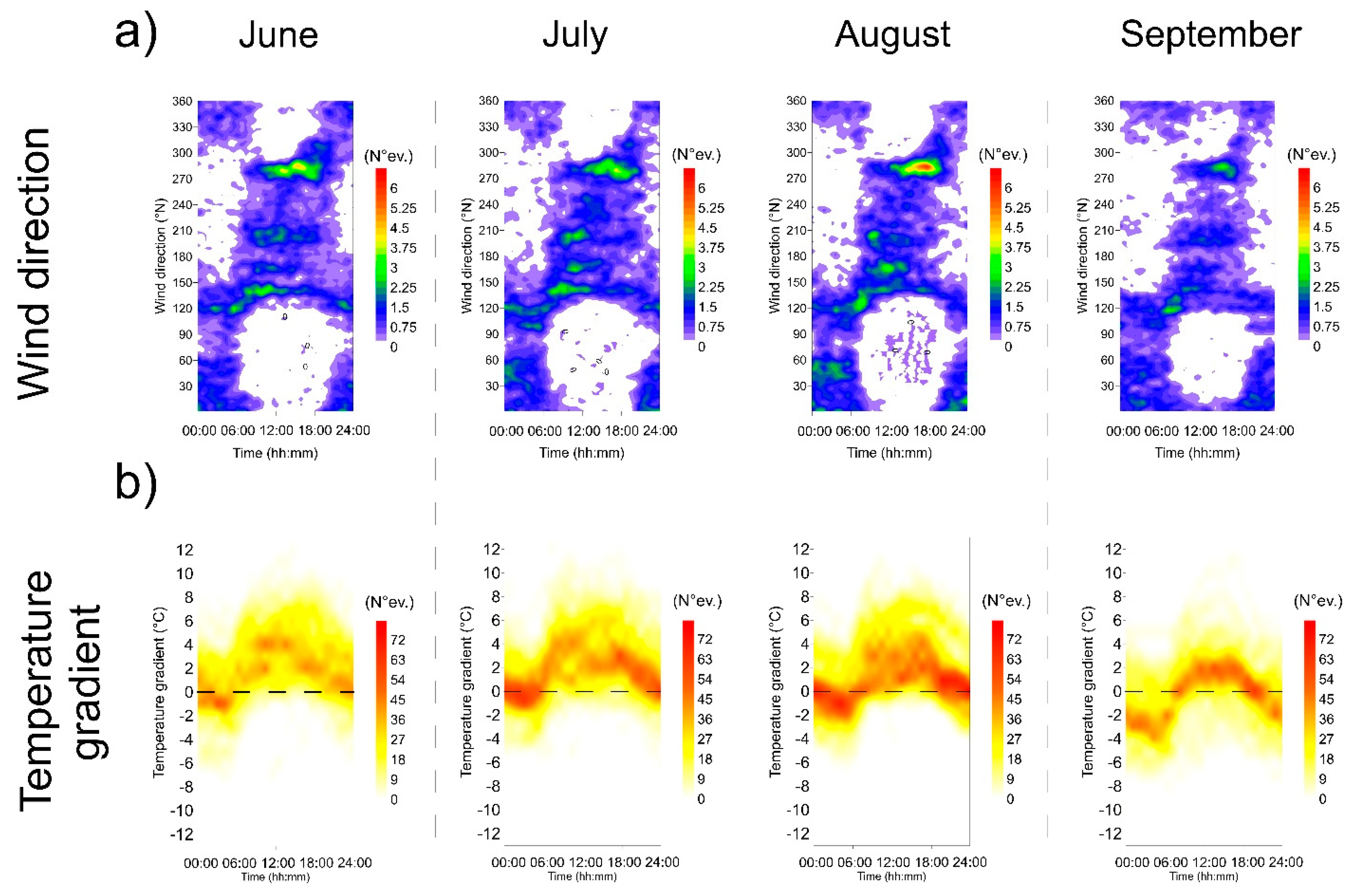
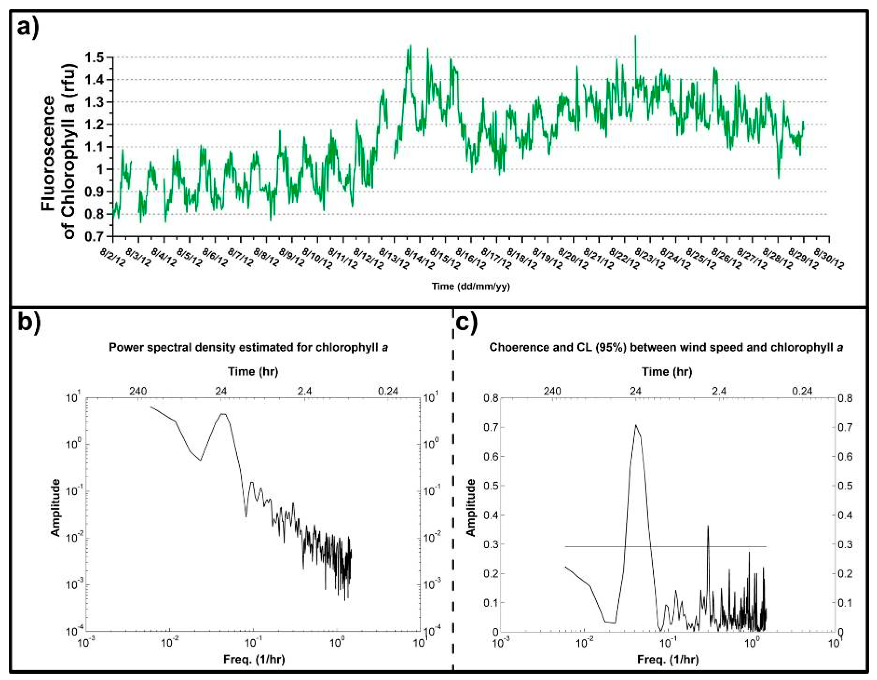
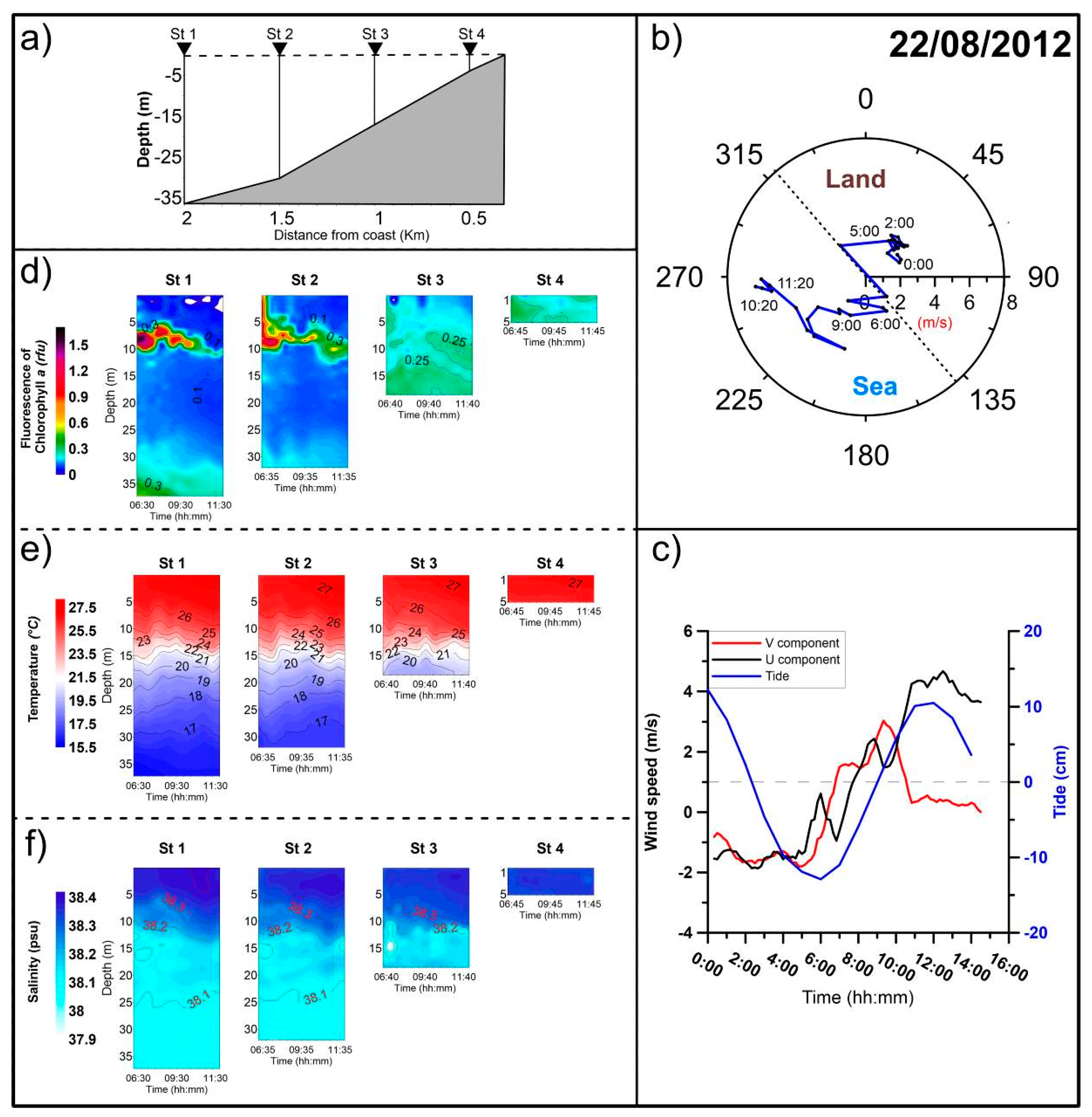
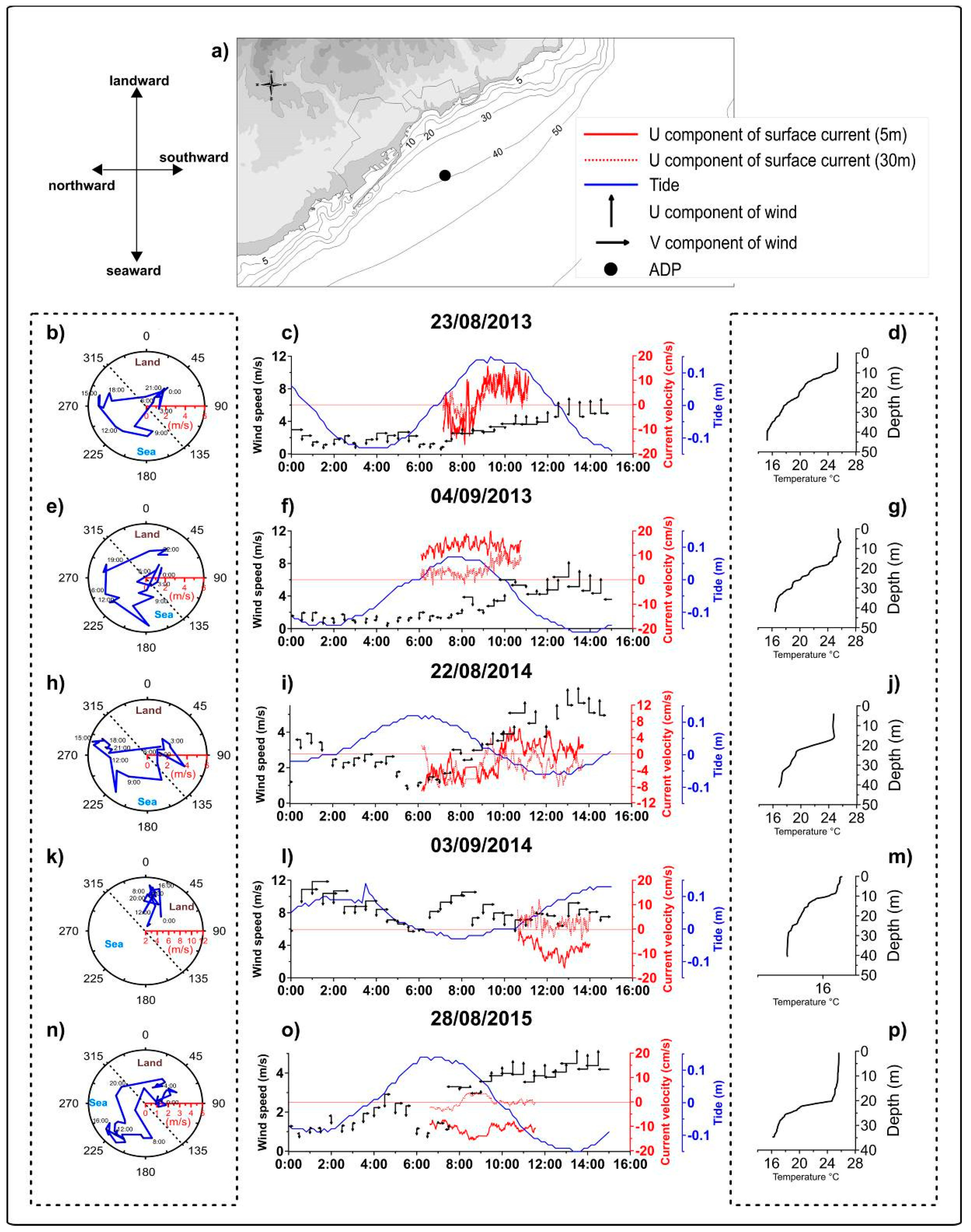
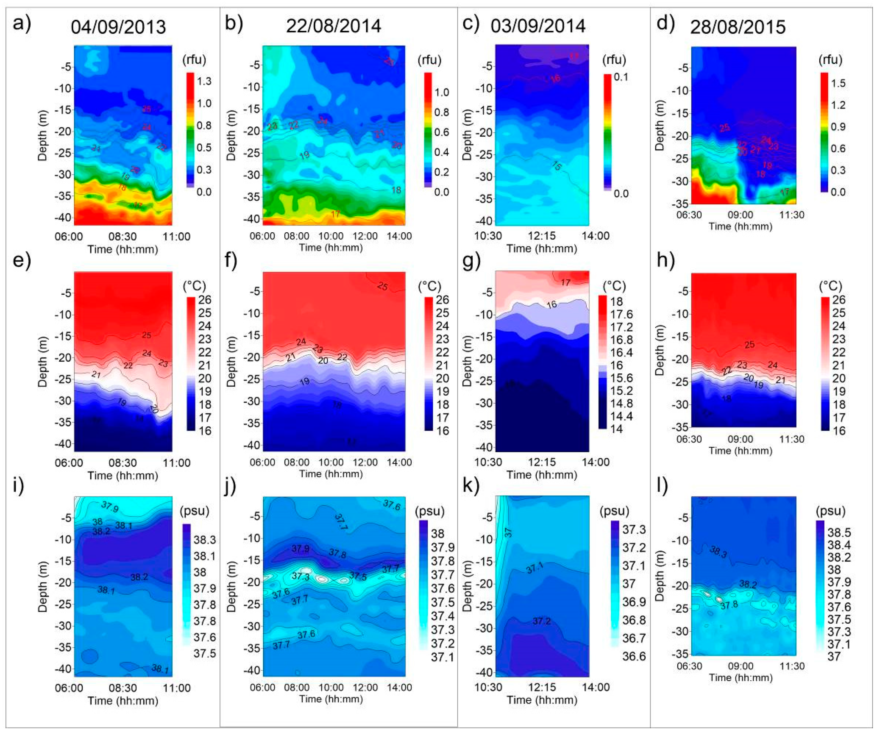
3.2. Fixed Point Survey: Highlights Coastal Currents, Fluorescence Patch, and the Physical Characteristics of the Sea Water over Time

In Figure 6c,f,i,l,o, the results of ADCP surveys, performed between 2013 and 2015, are correlated to wind and tide, forcing us to better understand the dynamical process, emphasizing the cross-shore component dynamic of coastal circulation.
The results of the survey of 23 August 2013 (Figure 6b,c) show weak NE wind during the night (2–3 m∙s−1) which quickly reverses from 7:00 to S, progressively increasing its speed. This reflects on the cross-shore components of wind which are also first oriented seaward and then landward. In particular, the cross-shore component of wind strengthens during the day. During ADCP measurements, the tide is in the raising phase, and circulation shows a well evident turnover which involves the whole water column of cross-shore component being in agreement with the rotation of the wind. On the surface layer, the temperature has a value of 25 °C (Figure 6d). The water column’s thermal structure shows a strong stratification over 10 m depth, with the temperature decreasing gradually to 15.5 °C in the bottom layer.
The survey of 4 September, 2013 (Figure 6e,f) is characterized by offshore weak winds (<2 m∙s−1) that were subjected to progressive rotation and strength during the day. Cross-shore components of the wind are seaward oriented and reverse from 7:00. The tide (Figure 6f) raised during the day, reaching the maximum at 8:00. According to the landward flux of raising tide, cross-shore components of currents are uniform and landward oriented during sampling time. Water column thermal structure (Figure 6g and Figure 7e) shows a mixed layer until 20 m depth, with a temperature of about 25 °C. Between 20 and 22 m depth, a higher temperature gradient is observed, with temperature decreasing from 24 °C to 22 °C. Moreover, the isotherms in this layer present an oscillation, characterized by three different peaks (Figure 7e). Below this layer, close to the bottom, temperature decreases to 16 °C. Over time, an increase of 2.5 °C is observed until 25 m depth. This is characterized by sloping downward isotherms, with the 19 °C isotherm deepened from 28 m to 32 m. Close to the bottom temperature increase is about 0.5 °C. In regards to salinity structure (Figure 7i), the surface layer presents a lower value of about 37.9 psu, which subsequently shrinks up to 5 m depth. At a depth between 10 and 20 m, high salinity is observed, with values of about 38.2 psu. Below 20 m of depth, salinity has values of 38 psu, showing a sinking similar to what is seen in temperature (Figure 7e). In the deep layers, values of FChla are the highest (1.2 rfu), while in the surface layers, the values are less than 0.2 rfu. The fluorescence deep patch follows the isotherm arrangement, highlighting the sinking of water (Figure 7a). The mixed layer shows low values of FChla, which further decreases up to complete disappearance over time.
The meteorological conditions on 22 August 2014 (Figure 6h,i) are variable during the day, showing several changes in wind direction and a progressive increase of wind speed from 8:00. At first, the cross-shore component of the wind (Figure 6i) was seaward oriented, while from approximately 7:00, it turned landward, increasing its strength progressively. The tide cycle reached its maximum at 6:00 with minimum levels at 12:00, during which ADP measurements were done. The circulation is characterized by an evident turnover of cross-shore components of surface currents. This was not followed by changes in the bottom currents, which remain offshore oriented. The bottom currents seem to be driven by the effect of lowering tide, while at the surface, the turnover is in agreement with wind. The hydrographical conditions (Figure 6j and Figure 7f) show a stratified water column. This has a definite thermocline that is characterized by tight isotherms of roughly 19 to 25 °C centered near the 22 °C isotherm and a surface layer that is characterized by a temperature of 24.5 °C and a depth of about 20 m. In proximity to the thermocline, the isotherms present oscillations from the horizontal plane: at 9:00, the 24 °C isotherm is at 16 m of depth, two hours later it is at 21 m of depth, and at 12:00, it is at 18 m of depth. Below the 20 °C isotherm, the temperature gradually decreases to 16.5 °C close to the bottom. The 18 °C isotherm are sloping upward until 10:30 and then downward. On the bottom layer, it is possible to observe a thermal increase of about 0.5 °C.
The surface layer presents a salinity of about 37.7 psu up to 15 m of depth (Figure 7j). Below this, a layer of approximately 5 m thickness is observed, characterized by a higher salinity of about 38 psu. This layer has an oscillation that initially lifts up to 10 m depth (8:00) and later on sinks down to a depth of 20 m. Below this, another layer was identified with significantly lower salinity of about 37.2 psu which follows the oscillations of the layer above. At greater than 25 m depth, salinity down to the bottom presents homogeneous values of 37.7 psu; 37.7 isohaline shows the same trend of the 18 °C isotherm. FChla values in the surface layer were first about 0.5 rfu, and later showed a distinct decrease, with near-zero values (Figure 7b). On the thermocline, the FChla shows the same oscillation of isotherm. The layers below the thermocline have values ranging from 0.7 rfu to 1.1 rfu, with the latter being found in the bottom layer. At the 18 °C isotherm, the FChla decreases rapidly between 10:00 and 10:30.
During the survey on 3 September, 2014 (Figure 6k,l), the constant moderate wind from NE determined the all-day-long dominance of southward components of wind with a minor cross-shore component seaward-oriented. The ADP measurements (Figure 6l) were performed during the increasing phase of the tide and results show a landward orientation of cross-shore components of currents at the bottom, while at the surface, the cross-shore motion is seaward. Moderate intensity and constant wind direction constrain surface circulation seaward with a consequent landward flux at the bottom, in accordance to the typical dynamic of the upwelling condition [56]. Water column in Figure 6m shows low temperature (≈16 °C) that is atypical during the summer season. The water column is well mixed up to the bottom and the presence of a thermocline is not observed (Figure 7g). The distance between an isotherm and the other is greater than 10 m. The isotherm of 15 °C sinks to about 10 m with an initial depth of 25 m, which after about 3 h, lowers to 35 m. Salinity presents a variation between the surface and the bottom of 0.2 psu. On the surface, lower values of 37 psu are observed. The distribution of FChla along the water column (Figure 7c) presents extremely low values comprised between 0 and 0.1 rfu, with the largest values found in the deeper layers (1 rfu).
During the survey on 28 August 2015, the wind progressively increased together with a full rotation from NE to SW. This rotation corresponded to a turnover of cross-shore components, first seaward and then landward (Figure 6n,o). From 1:00 to 13:00 on 28 August 2015, a full tidal cycle was observed, with a sea level gradient of about 30 cm and the tide in lowering phase. The surface cross-shore components of the current was seaward during the whole sampling period without following the change in the direction of the wind. On 28 August 2015, the water column thermal structure (Figure 6p and Figure 7h) showed a mixed layer until 20 m depth, with a temperature of about 25 °C. Between 20 and 25 m of depth, an elevated thermal gradient of 6 °C was observed, characterized by tight isotherms of roughly 19 to 24 °C centered near the 22 °C isotherm. The isotherms present oscillations, noticeable between 06:30 and 9:30. Over 25 m depth, the temperature gradually decreases close to the bottom to 17 °C; 18 °C and 17 °C isotherms highlighted a shift of 5 m at 7:00. In Figure 7l, the mixed layer shows a salinity of about 38.3 psu. Below this, a layer of approximately 5 m thickness appears and is characterized by an elevated salinity gradient. The gradient ranges from 38.2 psu to 37.8 and presents the same oscillation observed in temperature (Figure 7h). Inside this layer, two areas that are characterized by a very lower salinity (37.1 psu) are observed, as it was seen on 22 August 2014 (Figure 7j). Over 25 m depth salinity presents homogeneous values of 37.8 psu. The mixed layer is also characterized by low values of FChla (Figure 7d). Over the thermocline, more elevated values are observed until 9:00. FChla shows a gradual increase, increasing from 0.6 rfu to 1.5 rfu in depth following the isotherm arrangement. After 09:00, the FChla disappears, with a subsequent increase up to 0.9 rfu until the 18 °C isotherm.

3.3. Gridded Survey: Shows the Fluorescence Patch and the Physical Characteristics of the Sea Water in a Large Area of the Study Domain

During the survey on 26 August 2016, the wind showed weak intensity and offshore direction during the night (Figure 8b). The land breeze had blown for about seven hours until 5:40 (started at 22:20 the day before), turning progressively offshore from 5:30 and strengthening from 9:00. The Wind Hodograph shows a clockwise rotation that is typical of a sea/land breeze regime. The tide cycle (Figure 8c) reached its minimum at 9:00 and reached the maximum at 16:00. During the survey, the wind had blown from 225° N and the tide was in the rising phase. The sea surface temperature that was recorded in WQMS (Water quality monitoring station) harbor (Figure 8a) highlights a rapid increase (>1 °C) between 9:00 and 11:00.
The near surface temperature that was recorded during the survey showed a coast-wide thermal gradient (Figure 8d). The four transect differ in the surface temperature and FChla distribution patterns (Figure 8e). In the northernmost transect, the 24.4 isotherm is between the 40 and 30 m isobaths, while in the southernmost, it is on the 10 m isobaths. The near surface FChla pattern presents the same characteristics that were observed in the temperature disposition, with the 0.5 chlorophyll a isoline disposition suggesting an advance in the distribution of the chlorophyll a patches towards the coast.

4. Discussion

General atmospheric conditions during the surveys were typical of the sea/land breeze regime, characterized by clockwise wind rotation, as observed clearly on the 22 August 2012. In the Mediterranean coastal area, there is a strong influence of sea/land breeze events during the year, especially in the summer season [30,31,32]. Previous findings highlighted a quick response of coastal surface currents to wind rotation [8,9] and an agreement between the direction of the wind and currents [14]. Furthermore, a complete observation of the water column dynamic during these events is missing from the literature. The complex terrains and the external forcing (e.g., cross-shore pressure gradient, sea surface temperature along and near the shore) play a role on sea/land breeze circulation [5,6,57]. These factors can modify the rotation of the wind, starting from its development from the ideal case [7]. An exception to the sea/land breeze condition is represented by the survey on 3 September, 2014, when the moderate northerly winds blow on the study area from the day before. This event caused a mixed water column with low temperature (≈16 °C). This is atypical during the summer season when the water column is stratified and the temperature is higher than 22 °C, suggesting the presence of an upwelling event [58]. Usually, the dynamic of the water column is characterized by a surface mixed layer with a thickness of 10 m and 20 m and an average temperature of 26 °C, a definite thermocline, which is characterized by tight isotherms and a stratified deep layer.
The phytoplankton patch has a general dynamic that follows the displacement of the isotherm and the higher concentration in the deep layer (>1 rfu), while in the mixed layer, the general low values of biomass quickly decrease during the first inversion of breeze circulation. The high concentration in the deep layer can be attributable to aggregated death cells that are residual of spring bloom which sink below the thermocline, remaining confined in the deep layer during summer [59,60]. These patches are probably diatoms that grow in low light, low temperature, and high nutrients, with the latter usually higher in the deep layer during the summer season. On 22 August 2012, a patch confined near the thermocline that follows the movement of the isotherm presented high values of FChla concentration (1 rfu), suggesting that the presence of dinoflagellates is favored during elevated irradiance and low nutrient conditions.
The current dynamic is coherent with the wind rotation, responding with a delay of a 4–5 h, which is in agreement with previous experiments [8,10,11,12,14]. This behavior is clearly evident on 23 August 2013 and on 22 August 2014, when the surface currents move offshore until 9:00 and then rotate in the opposite direction. The surface circulation is generally associated to a deep current that flows in the opposite direction (22 August 2014 and 28 August 2015). The role of microtidal excursion becomes important in the presence of weak winds. As shown in Figure 6c (23 August 2013), during comparable meteorological conditions, the increase of current speed is detected when the wind-driven landward flux correspond to raising tide. On the contrary, when the tide is opposite to the direction of the currents, the flow speed decreases (Figure 6i,f).
On the 22 and 28 August 2012, the survey measurements with the ADCP are not available; however, on these days, the wind was typical of the breeze condition that was observed in the other surveys. These results suggest that the current dynamics are similar in days in which the current meter data were performed and it is possible to identify current dynamics following the fluorescence patches movements.
On the 22 August 2012, the surface FChla patch that was observed in stations 1 and 2 decreased up to its disappearance, suggesting an offshore surface flow. Below a depth of 10 m, the decrease in temperature (isotherm sloping upward) and in FChla suggests an onshore transport that occurs with notable increases in FChla values and water temperature. Subsequently, a deep offshore transport, characterized by an increase of FChla concentrations in the deep layer, suggested a deep onshore flow similar to the behavior observed on 22 August 2014. These dynamics are not observed in stations 3 and 4.
On the 28 August 2012, the wind was stronger than on the 22nd of the same month, causing a faster response in water dynamics. Moreover, a decrease in FChla patches in the surface layer suggests an offshore surface flow. Below the thermocline, there was an evident decrease in temperature and FChla, suggesting a rapid onshore deep flow that was characterized by advection of FChla-poor water. Compared to 22 August 2012, this day highlighted fast and strong flows and, indeed, the FChla values decreased within approximately 2 h and the dynamic is observable at all stations.
This surface flow can also be deduced by observing the FChla time series that was recorded by oceanographic buoys. This series shows the higher phase during the hours when the solar radiation is higher. The described trend presupposes the absence of photolimitation processes and an increase in observed biomass. Based on this, it can be assumed that the observed biomass is passively transported from the current, tilting between the coast and the sea, justifying the high coherence between the wind and the chlorophyll.
As observed in Figure 8d,e, there is a progressive increase in surface temperature and FChla values towards the coast, showing the progress of the surface patches according to the wind direction. In addition, a rapid increase of the temperature series recorded in WQMS harbor was observed. This increase of about 1 °C, which takes place in just under 1 h, may be due to a warmer offshore water progressing to the coast rather than to the warming of the sea surface.
During the days of sea/land breeze, in proximity of the thermocline, the isotherm fluctuated as well the FChla signal. As observed elsewhere [21], these oscillations could be considered as internal gravity waves due to both tide and wind driven current, as well-stratified water columns support the formation of internal gravity waves. We hypothesize that the observed oscillations may be due to the surface and bottom current that flows in the opposite direction. Moreover, a cooling of the layers below the thermocline, with isopycnals sloping upward, suggested a colder water inlet [16].

5. Conclusions

The investigation performed by our laboratory revealed the great variability of the coastal system, which is forced by both tide and local winds. Local atmospheric circulation presents high instability in both speed and direction. Based on the observations made, we hypothesized sea/land breeze induced circulations. In the early morning, the land breeze blows, causing an offshore surface current which transports the near-surface plankton over the shelves. This generates, as a dynamic consequence, a deep onshore current to arise, which causes the bottom layer to sink. This sinking is caused by the pressure of the incoming overlying water flow which pushes the water below towards the bottom, causing it to sink.
During the day and in the presence of sea breeze, the surface current moves and transports the shallow phytoplankton patches near the coast. Below the thermocline, an onshore transport occurs with notable decreases in FChla values and an increase in water temperature (isopycnal sloping downward). Furthermore, our observations suggest that sea/land breeze-induced circulation, concurrently with the tide, in stratified water favors the formation of internal waves. This great variability affects current dynamics and water column structures, highlighting that physical processes in coastal water occur with high temporal and spatial variability, generating wind driven current and buoyancy-driven motions that influence the coastal phytoplankton patches.
The in-situ data provide valuable input for the modelling of coastal ecosystems, as well as the influence of the wind-driven dynamics on coastal systems in a wide range of spatial and time scales. Our surveys and analysis help to better understanding these coastal processes which are of great interest for environmental issues as well as for navigational purposes.

Supplementary Materials

Acquired data have been made available both via the LOSEM free data archive at http://www.oceaneers.it/?page_id=1028&lang=it and PANGAEA Data Archiving and Publication database at https://doi.pangaea.de/10.1594/PANGAEA.859527.

Author Contributions

R.M. conceived of the study and wrote the manuscript. R.M., A.P., F.P.d.M., and V.P. performed all the field measurements. R.M. and F.P.d.M. analyzed the data. R.M., C.M. and F.P.d.M. carried out the data analysis. V.P. and M.M. contributed to the conceptualization, manuscripts revision, and preparation. All authors have read and approved the final manuscript.

Funding

This research was supported by the Environmental Office of Civitavecchia Port Authority.

Acknowledgments

We are grateful for support from Gisueppe M. R. Manzella. In addition, the authors would like to express gratitude to Daniele Piazzolla and the staff of the Laboratory of Experimental Oceanology and Marine Ecology (DEB), University of Tuscia.

Conflicts of Interest

The authors declare no conflict of interest.

References

  1. Simpson, J.E. Sea Breeze and Local Wind; Cambridge University Press: Cambridge, UK, 1994. [Google Scholar]
  2. Haurwitz, B. Comments on the Sea-Breeze Circulation. J. Meteorol. 1947, 4, 1–8. [Google Scholar] [CrossRef]
  3. Pendergrass, W.R.; LaToya, M.; Vogel, C.A.; Bhaskar, V.; Dodla, R.; Dasari, H.P.; Yerramilli, A.; Baham, J.M.; Hughes, R.; Patrick, C.; et al. Observational Analysis and Modeling of the Sea Breeze Circulation during the NOAA/ARL—JSU Meteorological Field Experiment in Summer 2009. In Proceedings of the 15th Symposium on Meteorological Observation and Instrumentation, Savannah, GA, USA, 17–21 January 2010. [Google Scholar]
  4. Arrit, R.W. Effects of the Large Scale Flow on Characteristic Features of the Sea Breeze. J. Appl. Meteorol. 1993, 32, 116–125. [Google Scholar] [CrossRef]
  5. Johnson, A., Jr.; O’Brien, J. A study of an Oregon Sea Breeze Event. J. Appl. Meteorol. 1973, 12, 1267–1283. [Google Scholar] [CrossRef]
  6. Frenzel, C.W. Diurnal Wind Variations in Central California. J. Appl. Meteorol. 1962, 1, 405–412. [Google Scholar] [CrossRef] [Green Version]
  7. Neumann, J. On the rotation rate of the direction of the Sea and Land Breeze. J. Atmos. Sci. 1977, 34, 1913–1917. [Google Scholar] [CrossRef]
  8. Sonu, C.J.; Murray, S.P.; Hsu, S.A.; Suhayda, J.N.; Waddell, E. Sea breeze and coastal processes. EOS Trans. Am. Geophys. Union 1973, 54, 820–833. [Google Scholar] [CrossRef]
  9. Cianelli, D.; Uttieri, M.; Buonocore, B.; Falco, P.; Zambardino, G.; Zambianchi, E. Dynamics of a very special Mediterranean coastal area: The Gulf of Naples. In Mediterranean Ecosystems: Dynamics, Management and Conservation; Williams, G.S., Columbus, F., Eds.; Nova Science Publishers, Inc.: New York, NY, USA, 2011; Chapter 7; pp. 129–150. [Google Scholar]
  10. Vesecky, J.F.; Teague, C.; Daida, J.M.; Fernandez, D.M.; Onstott, R.G.; Hansen, P.; Laws, K.; Plume, M.A. Observations of currents from the near-surface to 50 m depth using a new multifrequency HF radar and an ADCP located in the radar observational area. In Proceedings of the 1998 IEEE International Geoscience and Remote Sensing Symposium Proceedings (IGARSS’98), Seattle, WA, USA, 6–10 July 1998; Volume 1, pp. 195–197. [Google Scholar] [CrossRef]
  11. Winant, C.D.; Beardsley, R.C. A comparison of Some Shallow Wind-Driven Currents. Notes and Correspondence. J. Phys. Oceanogr. 1979, 9, 218–220. [Google Scholar] [CrossRef]
  12. Woodson, C.B.; Eerkes-Medrano, D.I.; Flores-Morales, A.; Henkel, S.K.; Hessing-Lewis, M.; Jacinto, D.; Needles, L.; Foley, M.M.; Nishizaki, M.T.; O’Leary, J.; et al. Local Diurnal Upwelling driven by sea breezes in Northern Monterey Bay. Cont. Shelf Res. 2007, 2718, 2289–2302. [Google Scholar] [CrossRef]
  13. Hearen, H.; Millot, C. Seasonality of internal gravity waves kinetic energy spectra in the Ligurian Basin. Ocean. Acta 2003, 265, 635–644. [Google Scholar] [CrossRef]
  14. Menna, M.; Buonocore, B.; Zambianchi, E. Misure radar di correnti superficiali nel Golfo di Napoli. Proc. Ital. Assoc. Oceanol. Limnol. 2008, 19, 333–337. [Google Scholar]
  15. O’Donncha, F.; Hartnett, M.; Nash, S.; Ren, L.E. Characterizing observed circulation patterns within a bay using HF radar and numerical model simulations. J. Mar. Syst. 2015, 142, 96–110. [Google Scholar] [CrossRef]
  16. Pineda, J. Internal tidal bores in the nearshore: Warm-water fronts, seaward gravity currents and the onshore transport of neustonic larvae. J. Mar. Res. 1994, 52, 427–458. [Google Scholar] [CrossRef]
  17. Franks, P.J.S.; Walstad, L.J. Plankton patches at fronts: A model of formation and response to wind events. J. Mar. Res. 1997, 55, 1–29. [Google Scholar] [CrossRef]
  18. Franks, P.J.S.; Chen, C. Plankton production in tidal fronts: A model of Georges Bank in summer. J. Mar. Res. 1996, 54, 631–651. [Google Scholar] [CrossRef]
  19. Jones, B.H.; Halpern, D. Biological and physical aspects of a coastal upwelling event observed during March-April 1974 off northwest Africa. Deep Sea Res. 1981, 28A, 71–81. [Google Scholar] [CrossRef]
  20. Walsh, J.J.; Whitledge, T.E.; Kelley, J.C.; Huntsman, S.A.; Pillsbury, R.D. Further transition states of the Baja California upwelling ecosystem. Limnol. Oceanogr. 1977, 22, 264–280. [Google Scholar] [CrossRef]
  21. Lennert-Cody, C.E.; Franks, P.J.S. Fluorescence patches in high-frequency internal wave. Mar. Ecol. Prog. Ser. 2002, 235, 29–42. [Google Scholar] [CrossRef]
  22. Legendre, L.; Demers, S. Towards dynamic biological oceanography and limnology. Can. J. Fish. Aquat. Sci. 1984, 41, 2–19. [Google Scholar] [CrossRef]
  23. Kiørboe, T.; Nielsen, T.G. Effects of wind stress on vertical water column structure, phytoplankton growth, and productivity of planktonic copepods. In Trophic Relationships in the Marine Environment, Proceedings of the 24th European Marine Biology Symposium, Oban, UK, 4–10 October 1989; Aberdeen University Press: Aberdeen, UK, 1990; pp. 28–40. [Google Scholar]
  24. Dickey, T.D. The emergence of concurrent high-resolution physical and bio-optical measurements in the upper ocean and their applications. Rev. Geophys. 1991, 29, 383–414. [Google Scholar] [CrossRef]
  25. Franks, P.J.S. Phytoplankton Blooms at Fronts: Patterns, Scales, and Physical Forcing Mechanisms. Rev. Aquat. Sci. 1992, 6, 121–137. [Google Scholar]
  26. Traganza, E.D.; Redalje, D.G.; Garwood, R.W. Chemical flux, mixed layer entrainment, and phytoplankton blooms at upwelling fronts in the California coastal zone. Cont. Shelf Res. 1987, 7, 89–105. [Google Scholar] [CrossRef]
  27. Largier, J.L.; Lawrence, C.A.; Roughan, M.; Kaplan, D.M.; Dorman, C.E.; Kudela, R.M.; Bollens, S.M.; Wilkerson, F.P.; Dever, E.P.; Dugdale, R.C.; et al. WEST: A northern California study of the role of wind-driven transport in the productivity of coastal plankton communities. Deep Sea Res. II 2006, 53, 2833–2849. [Google Scholar] [CrossRef] [Green Version]
  28. Rau, G.H.; Ralston, S.; Southon, J.R.; Chavez, F.P. Upwelling and the condition and diet of juvenile rockfish: A study using C14, C13 and C15N natural abundances. Limnol. Oceanogr. 2001, 46, 1565–1570. [Google Scholar] [CrossRef]
  29. Margalef, R.; Estrada, M.; Blasco, D. Functional morphology of organisms involved in red tides, as adapted to decaying turbulence. In Toxic Dinoflagellate Blooms; Taylor, D.L., Seliger, H.H., Eds.; Elsevier/North Holland: New York, NY, USA, 1969; pp. 89–94. [Google Scholar]
  30. Leuzzi, G.; Monti, P. Breeze analysis by mast and sodar measurements. Il Nuovo Cimento C 1997, 20, 343–359. [Google Scholar]
  31. Mastrantonio, G.; Petenko, I.; Viola, A.; Argentini, S.; Coniglio, L.; Monti, P.; Leuzzi, G. Influence of the synoptic circulation on the local wind field in a coastal area of the Tyrrhenian Sea. Earth Environ. Sci. 2008, 1, 012049. [Google Scholar] [CrossRef] [Green Version]
  32. Petenko, I.; Mastrantonio, G.; Viola, A.; Argentini, S.; Coniglio, L.; Monti, P.; Leuzzi, G. Local Circulation Diurnal Patterns and Their Relationship with Large-Scale Flows in a Coastal Area of the Tyrrhenian Sea. Bound.-Layer Meteorol. 2011, 139, 353–366. [Google Scholar] [CrossRef]
  33. Caballero, R.; Lavagnini, A. A numerical investigation of the sea breeze and slope flows around Rome. Il Nuovo Cimento C 2002, 25, 287–304. [Google Scholar]
  34. Monti, P.; Leuzzi, G. A numerical study of mesoscale airflow and dispersion over coastal complex terrain. Int. J. Environ. Pollut. 2005, 25, 239–250. [Google Scholar] [CrossRef]
  35. Gariazzo, C.; Silibello, C.; Finardi, S.; Radice, P.; Piersanti, A.; Calori, G.; Cucinato, A.; Perrino, C.; Nussio, F.; Cagnoli, M.; et al. A gas/aerosol air pollutants study over the urban area of Rome using a comprehensive chemical transport model. Atmos. Environ. 2007, 41, 7286–7303. [Google Scholar] [CrossRef]
  36. Elliot, A.J. Low frequency current variability off the West coast of Italy. Oceanol. Acta 1981, 4, 47–55. [Google Scholar]
  37. Elliot, A.J.; de Strobel, F. Oceanographic conditions in the coastal water of NW Italy during the spring of 1977. Boll. Geofis. Teor. Appl. 1979, 20, 251–262. [Google Scholar]
  38. Hopkins, T.S. Recent observation on the intermediate and deep water circulation in the southern Tyrrhenian Sea. Oceanol. Acta 1988, 9, 41–50. [Google Scholar]
  39. Pinardi, N.; Navarra, A. Baroclinic wind adjustment processes in the Mediterranean Sea. Deep Sea Res. II 1993, 40, 1299–1326. [Google Scholar] [CrossRef]
  40. Pierini, S.; Semioli, A. Wind-driven circulation model of the Tyrrhenian Sea area. J. Mar. Syst. 1998, 18, 161–178. [Google Scholar] [CrossRef]
  41. Vetrano, A.; Napolitano, E.; Iacono, R.; Schroeder, K.; Gasparini, G.P. Tyrrhenian Sea Circulation and water mass fluxes in spring 2004: Observations and model results. J. Geophys. Res. 2010, 115, C06023. [Google Scholar] [CrossRef]
  42. La Monica, G.B.; Raffi, R. Morfologia e Sedimentologia della Spiaggia e della Piattaforma Continentale Interna; Borgia, T., Ed.; Regione Lazio Assessorato Opere e Reti di Servizi e Mobilità; Il Mare del Lazio, Università degli Studi di Roma “La Sapienza”: Roma, Italy, 1996; pp. 62–105. [Google Scholar]
  43. Anselmi, B.; Benvegnu, F.; Brondi, A.; Ferretti, O. Classificazione geomorfologica delle coste italiane come base per l’impostazione di studi sulla contaminazione marina. In Proceedings of the Atti III Congresso A.I.O.L., Sorrento, Italy, 18–20 December 1978. [Google Scholar]
  44. Brondi, A.; Ferretti, O.; Anselmi, B.; Falchi, G. Analisi granulometriche e mineralogiche dei sedimenti fluviali e costieri del territorio italiano. Boll. Soc. Geol. Ital. 1979, 98, 293–326. [Google Scholar]
  45. Scanu, S.; de Mendoza, F.P.; Piazzolla, D.; Marcelli, M. Anthropogenic impact on river basins: Temporal evolution of sediment classes and accumulation rates in the northern Tyrrhenian Sea, Italy. Oceanol. Hydrobiol. Stud. 2015, 44, 74–86. [Google Scholar] [CrossRef]
  46. Bakun, A.; Agostini, V.N. Seasonal Patterns of wind-induced upwelling/downwelling in the Mediterranean Sea. Sci. Mar. 2001, 65, 243–257. [Google Scholar] [CrossRef]
  47. Martellucci, R.; Pierattini, A.; Madonia, A.; Albani, M.; Melchiorri, C.; Piazzolla, D.; de Mendoza, F.P.; Bonamano, S.; Scanu, S.; Piermattei, V.; et al. Phytoplankton biomass distribution in water column and sediments in the northern Latium coastal area. In Proceedings of the 7th EuroGOOS Conference, Lisbon, Portugal, 28–30 October 2014. [Google Scholar]
  48. Martellucci, R.; de Mendoza, F.P.; Piazzolla, D.; Pierattini, A.; Marcelli, M. High resolution coastal monitoring during sea breeze events. In Proceedings of the SISC First Annual Conference, Lecce, Italy, 23–24 September 2013. [Google Scholar]
  49. Thompson, R.O.R.Y. Coherence significance levels. J. Atmos.Sci. 1979, 36, 2020–2021. [Google Scholar] [CrossRef]
  50. Bonamano, S.; Piermattei, V.; Madonia, A.; de Mendoza, F.P.; Pierattini, A.; Martellucci, R.; Stefanì, C.; Zappalà, G.; Marcelli, M. The Civitavecchia Coastal Environment Monitoring System (C-CEMS): A new tool to analyse the conflicts between coastal pressures and sensitivity areas. Ocean Sci. 2015, 12, 87–100. [Google Scholar] [CrossRef]
  51. Askari, F. Multi-sensor remote sensing of eddy-induced upwelling in the southern coastal region of Sicily. Int. J. Remote Sens. 2001, 22, 2899–2910. [Google Scholar] [CrossRef]
  52. Poulain, P.-M.; Mauri, E.; Ursella, L. Unusual upwelling and current reversal off the Italian Adriatic coast in summer 2003. Geophys. Res. Lett. 2004, 31, L05303. [Google Scholar] [CrossRef]
  53. Witers, E. Upwelling control of positive interactions over mesoscale: A new link between bottom-up and top-down processes on rocky shores. Mar. Ecol. Prog. Ser. 2005, 301, 43–54. [Google Scholar] [CrossRef]
  54. McPhee-Shaw, E.E.; Siegel, D.; Washburn, L.; Brzezinski, M.; Jones, J.; Leydecker, A.; Melack, M. Mechanisms for nutrient delivery to the inner shelf: Observations from the Santa Barbara Channel. Limnol. Oceanogr. 2007, 52, 1748–1766. [Google Scholar] [CrossRef] [Green Version]
  55. Tapia, F.J.; Navarrete, S.A.; Castillo, M.; Menge, B.A.; Castilla, J.C.; Largier, J.; Wieters, E.A.; Broitman, B.L.; Barth, J.A. Thermal indices of upwelling effects on inner-shelf habitats. Prog. Oceanogr. 2009, 83, 278–287. [Google Scholar] [CrossRef]
  56. Kämpf, J.; Chapman, P. The Functioning of Coastal Upwelling Systems. In Upwelling Systems of the World; Springer: Berlin, Germany, 2016; Chapter 2; pp. 31–65. [Google Scholar]
  57. Bowers, L. The Effect of Sea Surface Temperature on Sea Breeze Dynamics along the Coast of New Jersey “Graduate Program in Oceanography”. Master’s Thesis, Rutgers University, New Brunswick, NJ, USA, 2004. [Google Scholar]
  58. Martellucci, R.; Melchiorri, C.; Costanzo, L.; Marcelli, M. On the presence of coastal upwelling along the northeastern Tyrrhenian coast. In Proceedings of the 19th EGU General Assembly (EGU2017), Vienna, Austria, 23–28 April 2017; p. 13767. [Google Scholar]
  59. Lazzara, L.; Innamorati, M.; Nuccio, C.; Mazzoli, A.R.; Ceccatelli, G. Popolamenti fitoplanctonici dell’arcipelago toscano in periodo estivo. Oebalia 1989, XV, 453–462. [Google Scholar]
  60. Innamorati, M.; Lazzara, L.; Nuccio, C.; Mori, G.; Massi, L.; Cherici, V. Il fitoplancton dell’alto Tirreno: Condizioni trofiche e produttive. In Proceedings of the Atti del 9° Congresso A.I.O.L., Santa Margherita Ligure, Italy, 20–23 November 1990; pp. 199–205. [Google Scholar]
Figure 1. (a) Map of the Tyrrhenian Sea with a part of the study area (in white). (b) Bathymetric map of the Northern Tyrrhenian east coast; the black polygon is the study area. (c) Topographic map of the coastal zone of Civitavecchia and the observatory system. (d) The location of the measurement stations.
Water 10 01673 g001
Figure 2. (a) Density plot of the daily distribution of the wind direction (2008–2014); the density plot was calculated for each degree and N° Ev. represents the number of events for the degree. (b) Air-sea thermal gradient during the summer months (2012–2014); the temperature gradient was calculated by subtracting the air temperature values, which were recorded at the weather station, from the sea temperature values that were recorded at the Water Quality Monitoring Station (Figure 1d).
Water 10 01673 g002
Figure 3. (a) Time-series of chlorophyll a between 2 August 2012 and 29 August 2012 recorded by oceanographic buoy (St. 1). (b) Power spectral density performed on chlorophyll a and (c) coherence between chlorophyll a and wind speed.
Water 10 01673 g003
Figure 4. (a) Station location scheme along the transect survey. (b) Wind hodograph and (c) U (black line) and V (red line) wind components and tide (blue line) on the survey day. (d) Time series of chlorophyll a fluorescence, (e) temperature, and (f) salinity at all stations.
Water 10 01673 g004
Figure 5. (a) Station location scheme along the transect survey. (b) Wind hodograph and (c) U (black line) and V (red line) wind components and tide (blue line) on the survey day. (d) Time series of chlorophyll a fluorescence, (e) temperature, and (f) salinity at all stations.
Water 10 01673 g005
Figure 6. (a) Station location scheme along the coast. Wind hodograph (b,e,h,k,n) and (d,g,j,m,p) temperature profile along the water column. (c,d,f,i,l) U current component at 5 m (red line) and U current component at 30 m (red dots line), wind components (black arrows), and tide (blue line) for the survey days.
Water 10 01673 g006
Figure 7. (a) Time series of Fluorescence of chlorophyll a (ad) expressed in rfu (relative fluorescence units), Temperature (eh), and Salinity (il) at station 1.
Water 10 01673 g007
Figure 8. Sea surface temperature (a) at WQMS harbor, wind hodograph (b) and tide (c). Maps of surface Temperature (d) and Fluorescence of chlorophyll a (e) during the 26 August 2016 survey.
Water 10 01673 g008
Table 1. Measurement strategies design using CTD (small instrument package contained an Idronaut 316 Plus multiparametric probe and a SeaPoint fluorometer) and ADCP (Acoustic Doppler Current Profiler) sampled parameters.
Measurement DayMeasurement TimeMeasurement StrategySampled Parameter
CTDADCP
20 August 201206:00–08:00Offshore transect (St. 1: 42.0827083N/11.7778383E; St. 2: 42.08385N/11.78378E; St. 3: 42.085011N/11.788541E; St. 4: 42.085766N/11.79377E)X
22 August 201206:30–14:00Offshore transectX
24 August 201206:00–11:00Offshore transectX
28 August 201206:00–09:00Offshore transectX
23 August 201306:30–10:30Moored at St. 1 (40 m isobath)XX
4 September 201306:00–11:00Moored at St. 1 (40 m isobath)XX
22 August 201406:20–14:00Moored at St. 1 (40 m isobath)XX
3 September 201410:40–14:00Moored at St. 1 (40 m isobath)XX
28 August 201506:30–11:30Moored at St. 1 (40 m isobath)XX
26 August 201609:30–12:30Gridded survey (Figure 8d,e)X

