A Methodology for the Design of RTC Strategies for Combined Sewer Networks


1
Aquafin NV, R&D, Dijkstraat 8, 2630 Aartselaar, Belgium
2
KU Leuven, Sustainable Chemical Process Technology TC, Technology Campuses Ghent and Aalst, Gebroeders De Smetstraat 1, 9000 Gent, Belgium
3
KU Leuven, Hydraulics Section, Kasteelpark Arenberg 40, 3001 Leuven, Belgium
*
Author to whom correspondence should be addressed.
Water 2018, 10(11), 1675; https://doi.org/10.3390/w10111675
Submission received: 18 September 2018
/
Revised: 21 October 2018
/
Accepted: 13 November 2018
/
Published: 16 November 2018
(This article belongs to the Section Urban Water Management)
Abstract
:While real-time control (RTC) is considered an established means of performance improvement for existing urban drainage networks, practical applications are frequently only documented for large case studies, and many operators are still reluctant to adopt RTC into their own systems. The purpose of the presented study is to highlight the potential of RTC also for smaller networks by the example of five representative catchments in Flanders, Belgium, and to demonstrate a novel methodology for the automated design of control strategies. This method analyses a given sewer network for the identification of suitable existing and new control locations. The gathered information is used in a second step for the design of control algorithms according to generic control concepts documented in the literature, such as e.g., “Equal Filling Degree”. The resulting RTC strategy uses sensible default parameters, and can form a starting point for further refinement through optimization or manual tuning. With a modelled total combined sewer overflow volume reduction of 20% to 50%, the created strategies showed generally good performance for the tested catchments. The method proved to be applicable for all tested networks. Its use for the real-life implementation of RTC is currently under way for 10 other Flemish cases.
1. Introduction
Real-time control (RTC) is a widely accepted means to improve the performance of existing urban drainage systems. Many literature sources stress the usefulness and cost-efficiency of RTC [1,2,3,4,5,6,7,8,9]. However, it remains difficult for wastewater operators to choose RTC procedures for the implementation into their own systems. RTC is frequently regarded as being too complex and too expensive for implementation without case-specific investigation [10].
A wide range of studies [2,4,11,12,13,14] on the application of RTC to existing infrastructure focus on the implementation of one single control concept to one single catchment. Only little documentation exists on the analysis of the suitability of RTC for given case studies and the analysis of reasons for said suitability. A literature study [15] lists 30 case studies in Germany making use of RTC, and stresses the importance of such summaries for wastewater operators in order to facilitate their own decision making for (or against) the consideration of RTC solutions.
Existing tools for the implementation of RTC [16,17] focus on screening for the evaluation of RTC potential. The German guideline for the planning of RTC of sewer networks [18] encourages the use of such tools for the ‘assessment of control worthiness’. Also a demonstration software for a hypothetic case study [19] is published in order to convince wastewater operators of the usefulness of RTC. For the design of the actual RTC procedure, however, only few details on the appropriateness of RTC procedures for sewer systems are given in literature.
Generically applicable rule-based control (RBC) concepts exist [2,4,20,21,22] such as e.g., “Equal Filling Degree” (EFD), which seeks to fill each subbasin of a catchment up to the mean of all filling ratios [2,4,20]. The concepts are implemented for single case studies, proving that they improve the situation for the selected case. A modelling study [20] compares identical control concepts for two virtual, simplified sewer networks. The finding that an EFD strategy leads to higher combined sewer overflow (CSO) volumes than in the uncontrolled base scenario contradicts the findings of many other studies [1,2,4,7]. This could either signify that the virtual case studies were not representative of the response of real systems to RTC, that the used networks were oversimplified, or that, indeed, EFD is not suitable for reducing CSO activity for the investigated network configurations. Several studies (e.g., [1,23]) compare one RBC control concept with one model-based predictive control (MPC) concept, and [24] compare RBC with a more complex approach based on fuzzy logic for the reduction of CSO volume based on simplified models representing rather small urban drainage systems. Findings generally indicate that both simple and complex control concepts achieve the objective. Preference is then frequently given to the simpler of the two approaches. This is the opposite for investigations covering large catchments, where more complex control procedures such as optimization-based algorithms and/or MPC outperform simpler approaches [5,25,26]. Similar comparisons based on detailed hydrodynamic models appear to be scarcely documented in the literature, one exception being [23]. Research where the same control concept has been applied to different case studies in order to verify its applicability to a wide range of cases and highlight its sensitivity to network characteristics could not be found.
Considerable effort is made on the design of the control procedure, especially for MPC (see e.g., [25] for an overview). Only more recently, concepts for systems analysis for the identification of actuator locations [2,27,28], automated data conversion from detailed hydrodynamic models to control models [29], and for the evaluation of the effectiveness of implemented RTC strategies [30,31], are introduced.
Despite all these efforts, there is still reluctance among wastewater operators to adopt RTC [32]. One possible reason for this is the lack of literature documenting the application of control concepts to different case studies in order to verify their applicability to a wide range of cases. Another can be seen in the general hesitance of operators towards new technologies, especially when entailing increased complexity and potential for system failure.
This paper addresses these issues by presenting a procedure for the design of robust and proven global RTC strategies for the reduction of CSO volumes in existing combined sewer networks. It is largely automated in order to provide less subjective results and higher reproducibility than manual implementations, and to allow for easy implementation of RTC strategies for future cases.
2. Materials and Methods
The proposed procedure for the design of RTC strategies for combined sewer networks is applied to five representative case studies in Flanders, Belgium, to allow for generic conclusions for comparable catchments in this area. The following sections cover the description of used case study data and a detailed outline of the methodology and its major steps, being:
- Identification of overflow locations
- Identification of control locations and
- Control algorithm design.
The implemented control strategies are analyzed with regards to parameter sensitivities and the effectiveness of RTC compared to performance variability due to model parameter uncertainty of the uncontrolled scenario for CSO and flood volume. Finally, the performance of each scenario is evaluated for 850 rain events of a historic, long-term rainfall series.
2.1. Case Study Catchment Characteristics
Five catchments of the River Nete basin in Flanders, Belgium, of mostly combined sewer systems that were previously analyzed using the PASST methodology for their RTC potential [16] were chosen representing different scores of RTC potential, as documented by [33]. These networks can be regarded as typical examples of Flemish urban drainage systems: urbanized, but with less than 10% in terms of catchment area size and population count compared to many case studies on RTC documented in the literature (e.g., [2,5,6,11]) rather small. The wastewater is conveyed towards the central wastewater treatment plant (WWTP) gravitationally, and by a considerable number of pumping stations (PS). Both offline and in-line storage exists throughout the system. Frequent hydraulic interaction between sewer system and numerous small receiving waters make an exact delineation of the catchment boundaries difficult. The characteristics of these catchments are summarized in Table 1.
All catchments are chosen from the same region in Flanders to avoid obvious differences in their characteristics. Networks of flat areas will respond differently to RTC than networks in mountainous areas—these differences have been discussed by [20], and it is not the intention to repeat the results here. Rather, this study strives to analyze the potential success of RTC strategies actually implemented into the modelling environment, and compare those amongst each other and to the RTC potential predicted by PASST.
2.2. RTC Strategy Design
The methodology for the design of RTC strategies consists of two major steps that are detailed in the following sections. The first step is the identification of controllable subbasins delineated by control locations and (in- or external) overflow locations. The data of these subbasins and their interconnections are used in a second step to design control algorithms.
2.2.1. Identification of Controllable Subbasins
As preparation for network analysis required for the application of the methodology, the manual definition of the system’s most downstream node is required. This could be either the downstream node of the WWTP influent works, or at a PS or an arbitrary node in the network. In all five case studies in the present work, it is the WWTP influent. This node is used as the starting point for further network analyses. Any hydraulic structures downstream of this node will be ignored. The rest of the procedure described in the following sections has been automated by a number of routines implemented in Matlab [36] using a comma-separated-value (CSV) file containing all network information exported from Infoworks. Final output of the routine is a number of text-based files that can be loaded back into Infoworks for modification of the network to introduce controllers and to import the created control algorithms.
Overflow Locations
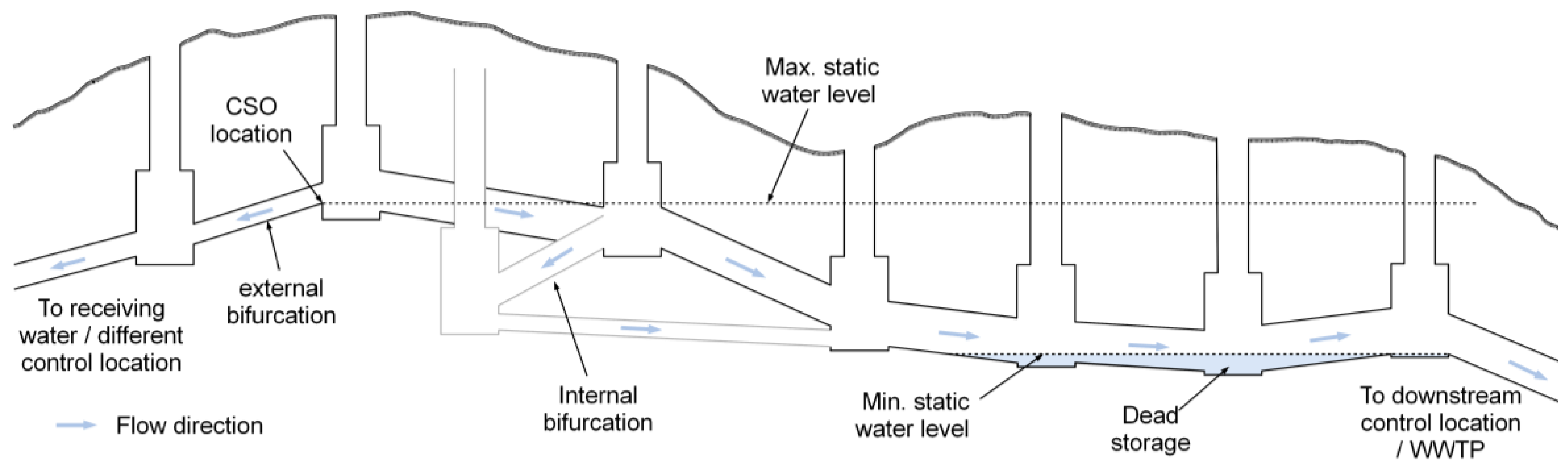
All network links are searched for overflow locations to ensure that parts of the receiving water that are included in the network can be identified, such that only the actual sewer system will be considered for the application of RTC. Overflow locations are, in this context, defined as links which separate all links with a hydraulic contribution towards the WWTP (actual sewer links) and the receiving water, i.e., any system outfall that is not defined as a treatment facility. The identification of such bifurcations is based on an algorithm originating in graph theory to allow for efficient calculation. Such algorithms analyze the network structure rather than actual simulation results, as, e.g., done by [37]. For an introduction of graph theory applied to sewer systems, see e.g., [38], who use graph theory for the identification of critical network elements with respect to system malfunctioning. The algorithm developed for the identification of overflow locations is illustrated in Figure 1.
The purpose of the algorithm is to determine the minimum water level required for each link to be drained either to the WWTP or another outfall (receiving water). This way, it is possible to assign flow directions to each link. Links with one node draining to the WWTP and another draining to the receiving water are considered external bifurcations, i.e., CSO locations. Internal bifurcations are not considered. A detailed flow chart of the algorithm is given in Figure A1. Once identified, overflow locations are considered a property of the given network that remains determined.
Control Locations
The identification of control locations allows more flexibility. Three automated options were considered in this study
- Using only existing control locations (E) such as PS or existing sluice gates. In the literature, this is frequently the case for studies investigating the control of PS [30,39,40,41,42] and other existing control locations, such as sluice gates [20]. In practical implementation, this might require the installation of new actuators, as existing gates might not be configured to handle frequent control actions.
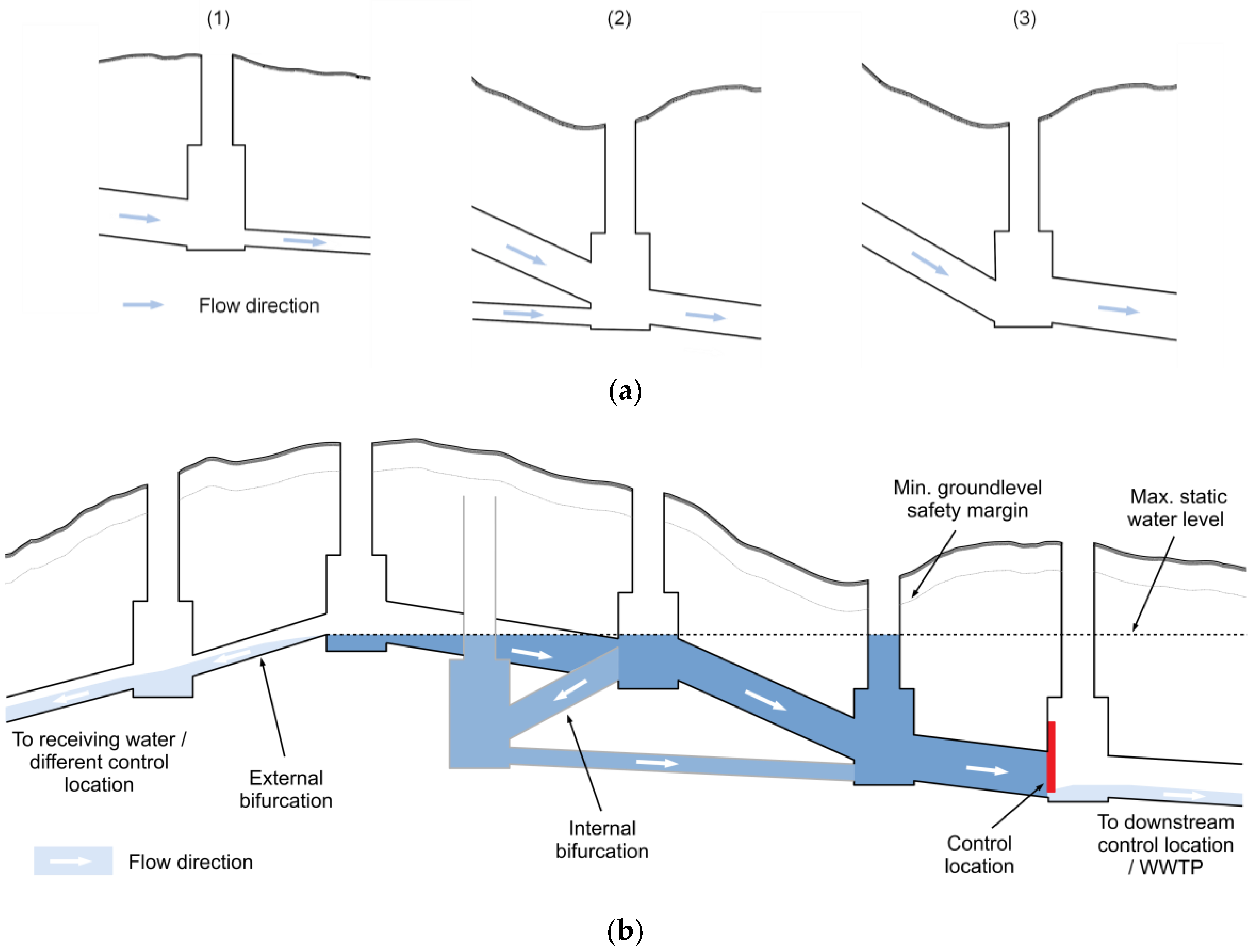
- Considering network links based on the individual flow capacity of these links (Q), assuming that links with significantly lower capacity than their upstream (US) and downstream (DS) neighbors form suitable locations for the installation of actuators [4]. Studies applying simplified models (e.g., [24,43,44,45,46]) often inherently use this approach, as they use ‘throttle devices’ as control locations, e.g., as outflow of storage basins. This approach can thus be seen as the one most frequently documented in literature. It relies on the assumption that existing flow limiters have been designed to activate a significant amount of storage volume. The control locations can be identified by comparing the flow capacities of all links US of a node vs all links DS of a node, as illustrated in Figure 2a. As control will most likely be active when the system is below its maximum capacity but water levels significantly exceed dry weather conditions, the influence of the energy gradient can be assumed to be negligible. Conduits can then be represented by their cross-section for this comparison; conduit slopes are ignored (see Figure 2a, case (3)).
- Selecting locations in a trunk sewer based on the in-sewer volume that can be activated in the collector upstream of the control location (V) [2]. This method is here extended to also take all side branches of the network into consideration. This appears to be of high relevance, as it has been shown in a case study [47] that the zone of backwater influence caused by actuators can be considerable, and indeed, may extend far into side branches. A further potential extension could include steady states for partially closed actuators, as suggested by [27]. As actuators in this study cannot be assumed to remain partially open, this extension is omitted here. As opposed to [27,28], the volume activated by a potential control location is not limited by bifurcations if these are drained towards the same potential control location as the sewer branch under consideration (see Figure 2b). This, again, is determined using the drainage levels discussed above. New locations are placed such that they are not influenced by backwater from downstream control locations.
In any of these cases, new actuators are only placed when the potentially activated control volume exceeds a threshold (chosen here: 100 m³). This effectively limits the number of control locations. The two latter approaches include the possibility of integrating existing actuators (e.g., PS) into the control strategy.
After the external bifurcations and control locations have been identified, the full delineations and all relevant properties of each subbasin (e.g., the number of people equivalents, storage characteristics, runoff surface area, etc.) are identified using the method proposed by [29].
This information can then be used to define new actuators at the downstream end of each subbasin that does not yet have an actuator, or to modify existing ones. Newly placed sluices are dimensioned according to the conduit at which they will be operating. They can be accompanied by overflow structures functioning as internal bypasses to ensure a controlled state of the system in case of malfunctioning of the actuators as e.g., implemented for existing case studies [47].
2.2.2. Control Algorithm Design
Each of the previously identified subbasins is considered as one unit to be controlled through its actuator (PS, sluice gate(s)). The actuators of the most downstream subbasin are controlled locally according to the requirements of the connected WWTP, as implemented in the base scenario. All other actuators are controlled globally in order to minimize the total CSO volume without increasing the total flood volume.
Most control algorithms applied in this study are global RBC algorithms. They can be straight-forwardly programmed into simple PLC (programmable logic controller) units, provided these can communicate amongst each other, and one of the devices can assume a coordinating function over the others. They have been reported to deliver good results (see e.g., [1,4,22]), and can thus be considered a good starting point for wastewater operators with limited experience of RTC. An overview on the control algorithms used in this study is given in Table 2.
Each control algorithm concept can be combined with any of the 3 choices for actuator positioning (existing, flow-based, volume-based), resulting in a total of 24 scenarios for each of the 5 models using RBC and 3 MPC scenarios for the network Arendonk.
All RBC algorithms rely on the concept of filling degree, the relative filling of a storage basin, or in-sewer storage with respect to a maximum level–usually the weir crest level of the lowest CSO of the subbasin or the lowest manhole ground level of the subbasin (including a safety margin) [1,2,4,7]. It strives at maximizing the storage activated in the sewer system by equally distributing storage activation over all subbasins of the sewer system. This is done by defining the setpoint for one subbasin by
- the mean of filling degrees over all subbasin (EQ glo), or
- the filling degree of the DS subbasin (DS loc), or
- the filling degree of the most DS subbasin (DS glo).
Local setpoint tracking is done either by two-point control (“on/off, “open/close”) as implemented by, e.g., [4], using a PID (proportional-integral-derivative) controller as is commonly applied in control engineering, or by mimicking the theoretical concept of the so-called central basin approach [48] by straightforward hydraulic calculations for the estimation of the flow at actuators required to empty the subbasin as quickly as possible into the DS subbasin, thereby
- aiming at filling the DS subbasin storage capacity up to a predefined maximum value (cs, see [22]) or
- using a desired discharge (qw) to the downstream basin as a means of negotiating a discharge that allows quickly emptying the upstream subbasin while considering downstream constraints and local boundaries for actuator flows and CSO activity (see [21]).
Flooding could be considered implicitly by all RBC algorithms for one location per subbasin where water level is monitored for the estimation of activated volume. As no such information is available for any other locations, no criteria for flooding have been implemented into the control algorithms.
Owing to the complexity of their application, algorithms making use of MPC using optimization rather than straightforward calculations of actuator setpoints are considered for only one of the case studies (Arendonk). Here, they serve as tests by which to evaluate whether the proposed methodology is applicable to MPC and, since MPC is frequently considered superior to RBC (see e.g., [25]), as a benchmark for the effectiveness of the applied RBC strategies. To ensure an objective comparison, it was decided to make use of existing MPC software. For this, an adapted draft version of the existing Matlab code DORA2 [6] has been used, which was made available by the authors of the software. As for the RBC algorithms, flooding is not considered explicitly by DORA2. As the hydrodynamic modelling environment Infoworks ICM does not allow for the exchange of information with the model during simulations, the model has been ported to SWMM [49] and re-calibrated based on simulation results of the Infoworks model. Communication between DORA2 and SWMM has been implemented using MatSWMM [50], available from GitHub [51].
2.3. Scenario Analyses
Global sensitivity analysis (GSA) has been applied to identify sensitive parameters of the designed control algorithms. To gain insight into the overall variability of CSO and flood volume as a result of parameter variation, and thus, the effectiveness of the applied RTC strategies, the results of this GSA are also compared to the uncontrolled scenario for each catchment for which 3 influential parameters have been varied within boundaries of reasonable uncertainty. Finally, each scenario is simulated using a long-term series of rainfall data in order to evaluate the variability of CSO and flood volume as a result of different rain event characteristics. The following sections give details on the applied evaluation criteria, GSA methodology, and used rainfall data.
2.3.1. Evaluated Criteria
When evaluating RTC, CSO volume is the most widely used criterion for emissions to receiving water in the scientific literature [25], as it combines easy determination, monitoring accuracy, and reliability. It will consequently also be used here as a means of performance evaluation.
Flooding is a criterion less frequently reported on [25]. However, as RTC might have widespread consequences on the hydraulic system behavior, flooding is considered as a secondary performance indicator in this study as recommended by [10]. It is calculated as the sum of the maximum flood volume for each flooding event recorded at all manholes. A more detailed investigation for flooding would have required a 2D surface flow modelling approach and model calibration based on reference data of real flood events, which were not available.
2.3.2. RTC Effectiveness and Parameter Sensitivity
Parameter sensitivity is here evaluated using Morris screening, a GSA method creating multiple one-at-a-time experiments. Parameter values are sampled with a uniform distribution from a predefined grid of possible values [52]. For each set of parameters, a simulation is run, and relative sensitivities with respect to the resulting total CSO and flood volume are calculated for each parameter that has been modified between 2 consecutive experiments. As proposed by [53], the mean absolute elementary effect (µabs) representing the mean of all absolute values of the relative sensitivities per parameter is here used as measure of parameter sensitivity. Convergence of the Morris screening, as defined by [54], was assumed to be reached when the variability of neither total CSO nor flood volume exceeded 5%.
For all scenarios using RTC, parameter boundaries are listed in Table 3 for the different setpoint tracking algorithms.
The results obtained from the sensitivity analysis are also used to evaluate the effectiveness of the applied RTC scenarios with regard to the reduction of total CSO volume and flooding compared to result variability of the uncontrolled scenario due to parameter uncertainty. To this end, additional scenarios have been evaluated for the uncontrolled scenario varying parameters not related to RTC within their uncertainty boundaries, as proposed by [30]. The selection of these model parameters and the chosen ranges listed in Table 4 are based on available literature [55].
2.3.3. Evaluation Period and Rainfall Data
All simulations have been carried out using data of one regional historical rainfall series with a temporal resolution of 1 min [56] (station ‘Herentals’). Spatial variability of rainfall has not been considered to ensure that all tested study areas receive the same rainfall input, and results can be compared among the catchments.
To allow for the high number of simulations required by the sensitivity analysis, a limited number of 24 rain events representative of different event return periods have been chosen. These represent 3% of the total 850 events, with a volume higher than 3 mm expected to have the potential for triggering CSO activity. They are concatenated such that each event is followed by a dry weather period long enough (here: 36 h for Arendonk and Wolfsdonk; 48 h for Beerse, Geel and Retie) to ensure that the entire sewer system reaches dry weather conditions before the beginning of the next event for any of the scenarios. Total rainfall event volumes range from 5.5 mm to 34.2 mm, and event durations from 100 min to 1268 min. Return periods depend on the aggregation (rainfall duration) used for event interpretation and vary from 0.07 years to 0.5 years for the lower bound and 0.1 years to 3 years for the upper bound.
As the performance of RTC scenarios is considered to be strongly dependent on the rain data [30], all scenarios with the parameterization leading to the best results for the short rainfall series were re-run using the full 13-year rainfall series in order to gain some insight in the actual CSO volume reduction and flooding behavior. For the MPC scenarios, perfect rainfall data prediction was assumed in order to consider the full theoretical potential of MPC.
3. Results
3.1. Storage Potential
The three different control location identification strategies (existing–E, flow-based–Q, volume-based–V) have been applied to all five networks. The resulting number of control locations and maximum total activated volumes are listed in Table 5.
The number of control devices strongly depends on the catchment and the applied strategy for the identification of control locations, with a very high correlation to total network pipe length (0.88 for existing, >0.9 for flow and volume). This is expected, as all networks have a considerable amount of in-sewer storage. For flow and volume-based identification, also contributing area (0.89, 0.99; existing: 0.42) and population count (0.75, 0.91; existing: 0.18) show a high correlation.
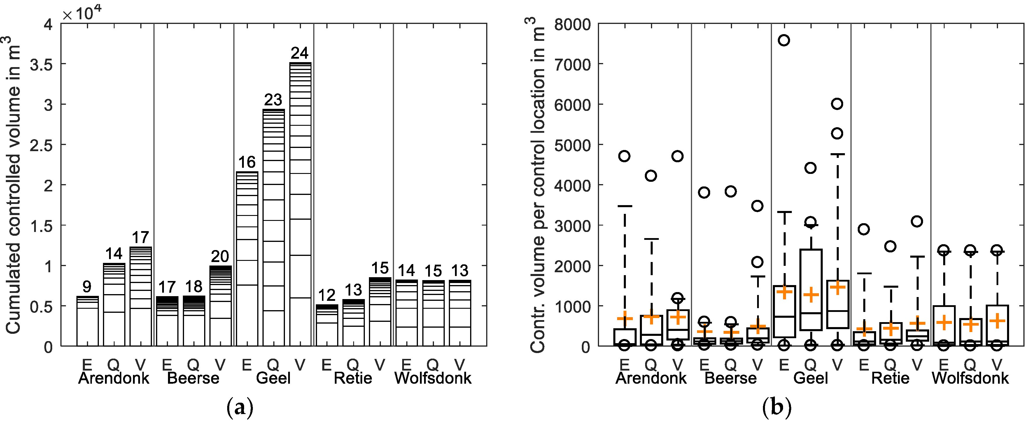
For four out of the five catchments, volume-based identification of control locations clearly shows the highest total control volume (Figure 3a). For one of the catchments (Wolfsdonk), the volume-based identification of control locations leads to the same overall control volume, but requires less control locations to do so. Arendonk shows an increase in total controlled volume by 65% and 100% for flow-based and volume-based identification, respectively. For Geel, these percentages are 30% and 60%. For Beerse and Retie, the increase by volume-based identification is around 60%. Flow-based identification shows no notable increase in controlled volume for these catchments. For Wolfsdonk, no effect is to be noted for either of the identification strategies. For all catchments, 30% to 50% of the total volume is controlled by one single control location when using only existing control locations (E). A large number of control locations is made up by existing PS with very small controlled volume. Both effects can be generally compensated for by any selection method of new control locations for the lager catchments Arendonk and Geel, but only through the application of volume-based control location selection for the smaller catchments of Beerse and Retie.
Interestingly, the identification of a higher number of control locations using the volume-based approach still leads to slightly higher average volume per control location when compared to both existing and flow-based locations (Figure 3b). This indicates a higher efficiency of the volume-based approach, while it appears that existing and flow-based choice of locations is predominant in literature (e.g., [4,24,30,39,40,41,42,43,45,46]), where the choice of control locations does not form an explicit research topic. It also means that general conclusions about the RTC potential based on the number of control locations alone should be refrained from: the positioning of the individual control locations within the network and with respect to each other is of high relevance. The highest average control volume per control location over all identification strategies is achieved for Geel, the largest of the investigated catchments featuring several long collectors with considerable storage potential. This is in line with literature stating that larger catchments show higher potential for the successful application of RTC [16,17].
3.2. RTC Effectiveness and Sensitivities
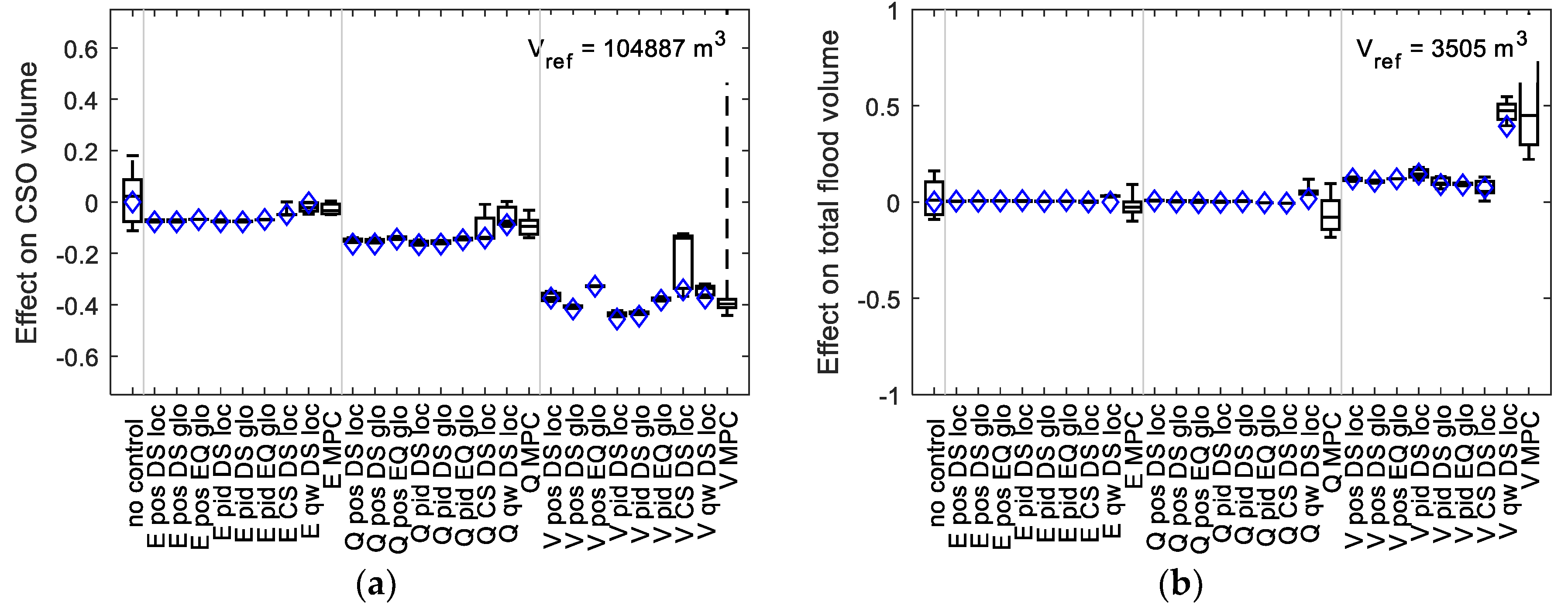
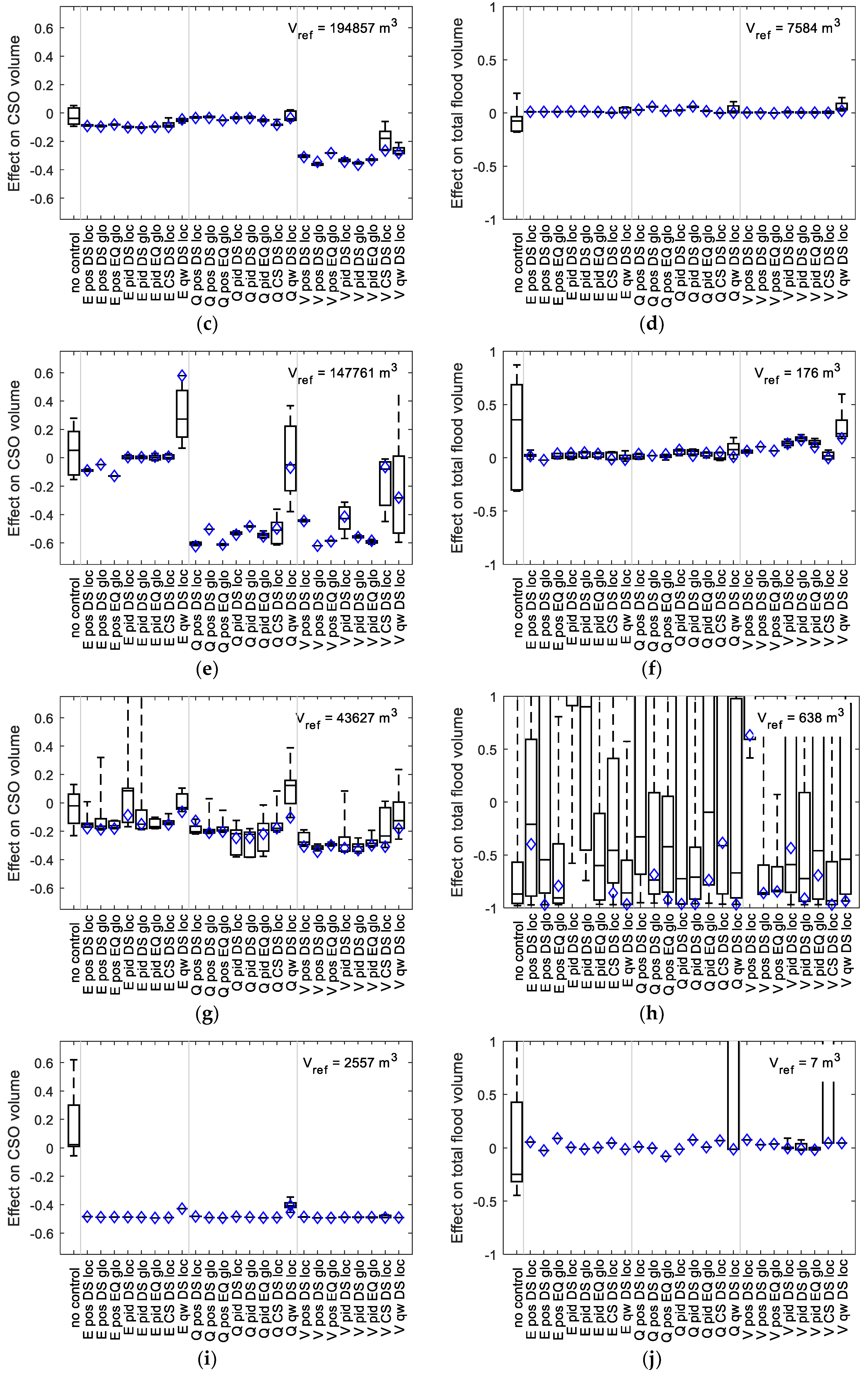
Figure 4 visualizes the results of the sensitivity analysis for the relative effect of the variation of parameters shown in Table 3 (RTC scenarios) and Table 4 (uncontrolled scenarios) on total CSO volume and total flood volume. It compares these effects for all control algorithms and catchments for the short series of selected rain events.
As can be seen, the influence of varying RTC parameters on total CSO volume is rather limited for most control algorithms using simple two-point or PID setpoint tracking. Compared to the range of results, even when using sensible default values for parameters rather than optimizing for each individual case, here leads to good results for Arendonk, Beerse, Geel and Wolfsdonk. Such default parameterization could thus form at least a sensible starting point for further analyses, as e.g., the suggested use for uncertainty analysis [30]. This, in turn, also means that control algorithms that perform worse than expected in their default parameterization (e.g., Arendonk V pos EQ glo) show very limited potential for improvement by modifying their (limited amount of) parameters. More complex algorithms (cs, qw) expectedly show a much higher sensitivity to their parameters. Surprisingly, however, they do not significantly outperform simple control, and in some cases, even show worse results for CSO volume.
Catchment Wolfsdonk shows almost no influence of any algorithm parameter on CSO and flood volume, while CSO volume is reduced by almost 50%. For Arendonk, Beerse, Geel, and Retie in combination with simple control algorithms, the choice of the control locations (E, Q, V) has a higher influence than control algorithm choice or algorithm tuning. Any control location scenario leads to improved CSO performance for well-parameterized control algorithms. The impact of using existing (E) control locations (in some cases up to 20% volume reduction), however, hardly exceeds the model uncertainty estimated for the uncontrolled network in these 4 catchments. Flow-based (Q) control location choice results in better results for Arendonk, Geel, and Retie: up to 60% CSO reduction for Geel and 15% to 30% for Arendonk and Retie. With at least 30% CSO volume reduction for all scenarios, the by far best results are achieved using the volume-based (V) choice of control locations.
Though anticipated for this research, the extent of the influence of the control location choice exceeded initial expectations for some cases. While the difference exhibited by Wolfsdonk and Geel is negligible and only small for Retie, for Arendonk and Beerse, the CSO volume reduction is doubled by moving from flow-based to volume-based selection of control locations. The large variability from catchment to catchment, even for the same control concept, highlights that the implementation of RTC to a specific case requires detailed analyses for the case in question, as advocated in literature [57].
Catchments Arendonk, Beerse, Geel, and Retie are all subject to some flooding for the short series of selected rain events. Wolfsdonk shows close to no flooding for any scenario. For Beerse, the catchment with the largest flood volume, hardly any influence is noticed for any of the control algorithms or choice of control location. Retie exhibits a very high sensitivity to control algorithm parameters. Also, the scenarios using volume-based control locations for Arendonk and Geel are susceptible to an increase in flood volume. When compared to the uncertainty estimation of the model, this is of no relevance for Geel, whereas for Retie it is possible to achieve a considerable reduction of the flood volume by control algorithm parameterization. For Arendonk, however, the modelled increase of the flood volume by several hundred m3 may require more in-depth investigations using a more accurate modelling approach (possibly 2D surface modelling) and more detailed rain data in order to ensure that a finally chosen RTC strategy will not result in an increased flood risk for this catchment. The potential for increased flooding could also indicate that there is no further potential for improvement of CSO volume performance for these scenarios.
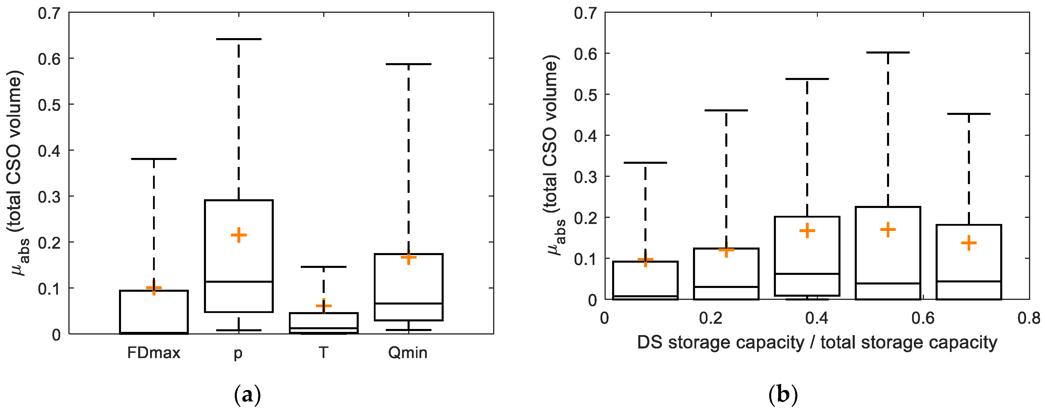
As is apparent from Figure 4, the control algorithm parameters analyzed for model sensitivity have only limited influence on the overall model results. However, a number of observations can be made based on the absolute elementary effects of parameters varied during the Morris screening (Figure 5): When averaged over all models (Figure 5a), local setpoint tracking parameterization using p and Qmin was shown to be influential, and good tuning of these values is required for optimal performance. This is unexpected, as scenarios ‘pos’ (using simple two-point-control) show equally good overall results. For qw scenarios, almost all tested cases show high sensitivity to qmin. Elementary effects for parameters FDmax and T, which have a physical meaning, are less prominent. This indicates that a sensible choice of default values for these parameters can be expected to lead to good performance for most cases. Calibration efforts should then focus on PID-controlled setpoint tracking and Qmin.
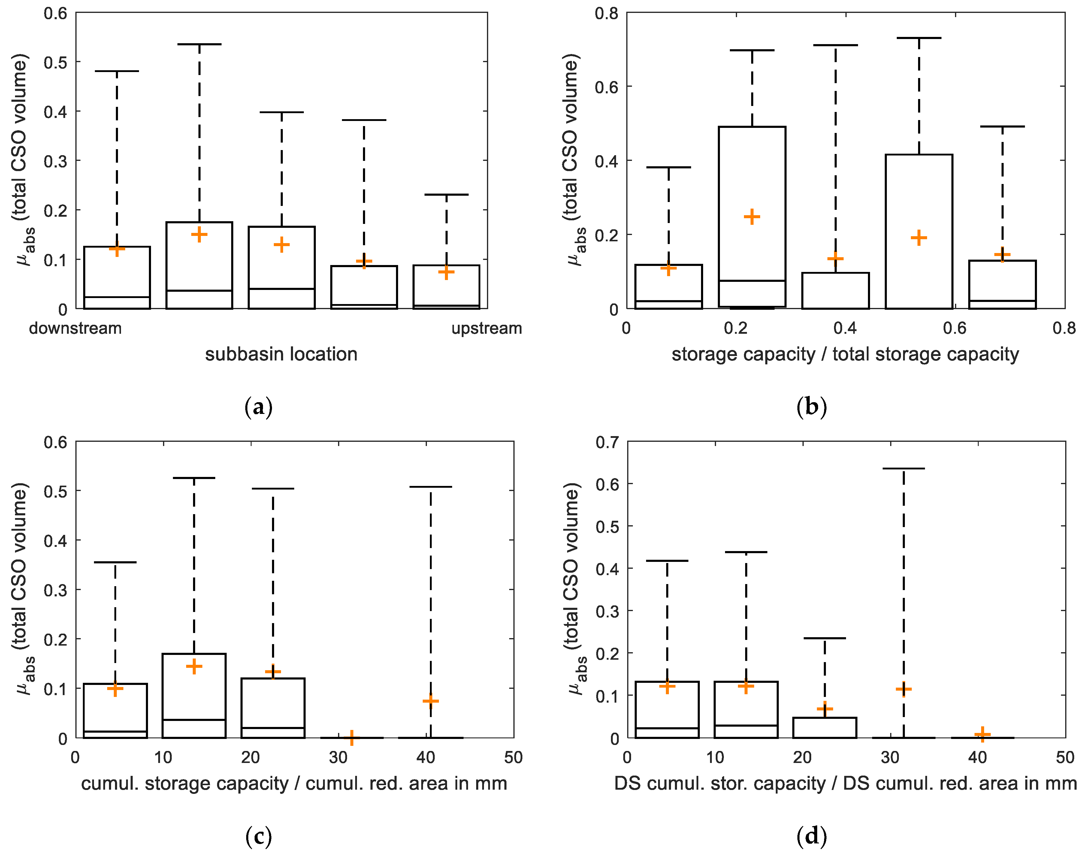
With respect to control location properties, only small correlations could be found for the resulting sensitivities. The relative storage capacity that can be activated by a control location as a fraction of the total storage capacity, for example, shows no correlation (see Figure A2) when analyzed for all control algorithms. The relative storage capacity of the subbasin downstream of the control location appears to have an influence on the sensitivity: Control locations with larger downstream catchments exhibit higher influence than others (Figure 5b), and should thus receive more attention during the fine-tuning of the algorithms.
3.3. Long-Term Simulations
The results obtained from the scenario analyses have been used to parametrize all control algorithms to run one final simulation using the full 13-year rainfall series for each network and control location choice. Results were analyzed for all 850 individual events.
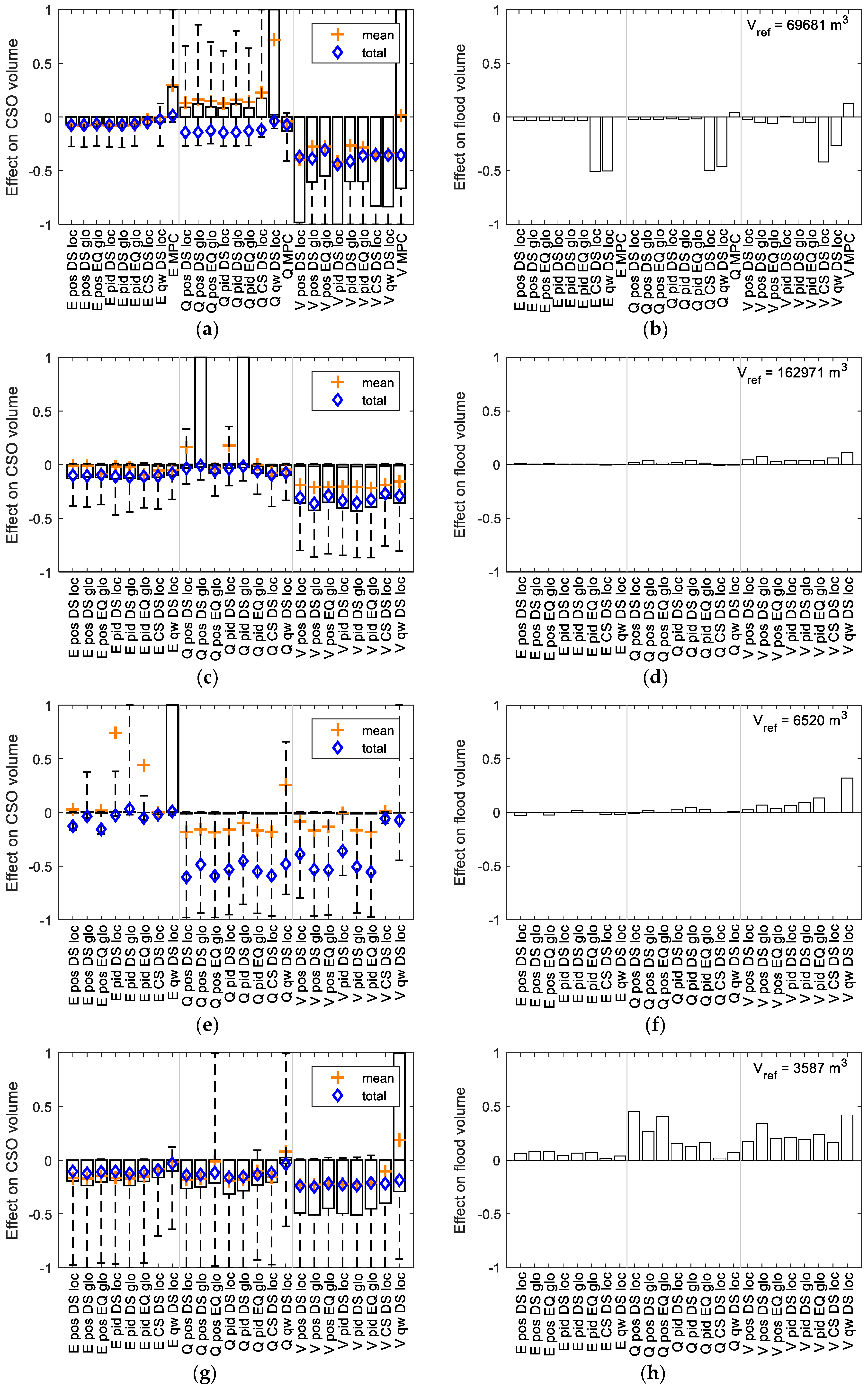
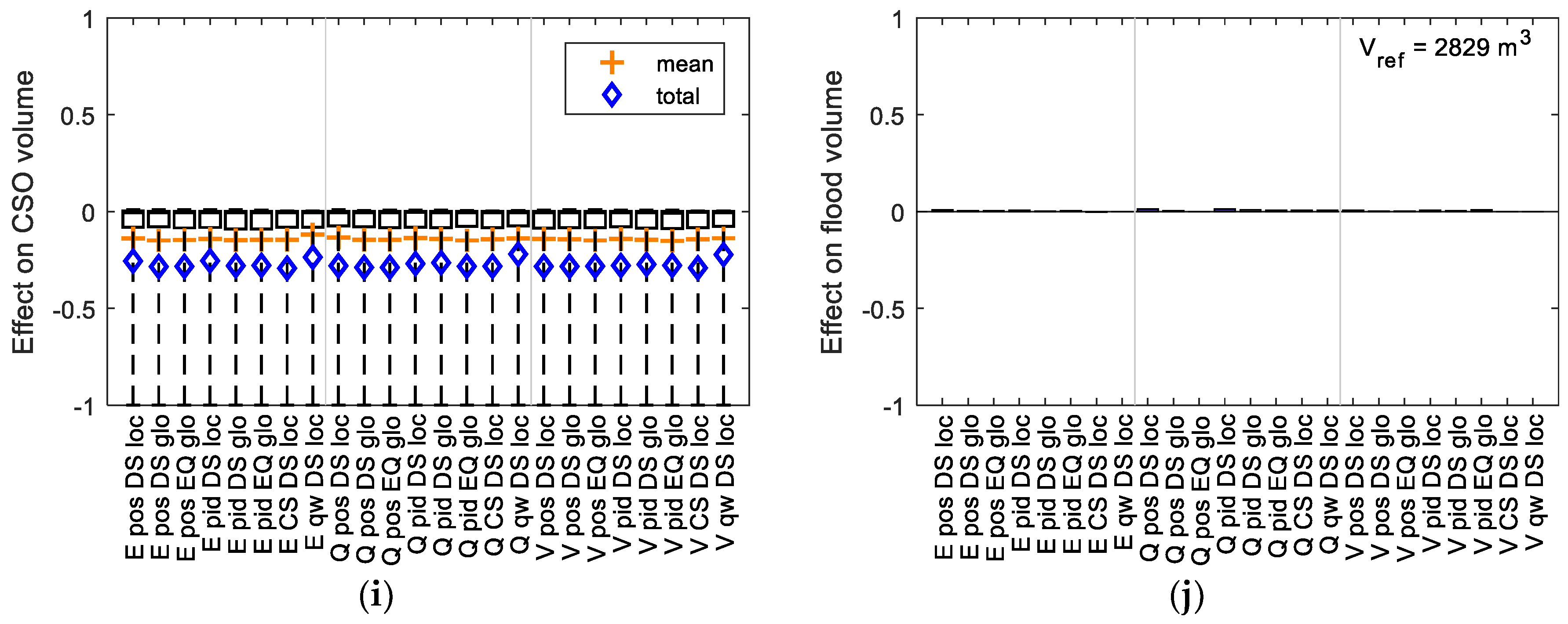
For total CSO volume, the results for these simulations, as shown in Figure 6, largely corroborate the findings of the scenario analysis: The choice of control locations has a dominant influence on CSO volume with volume-based selection outperforming flow-based and existing location choice. Also, differences resulting from control algorithm choice are small; more complex algorithms do not lead to better results for total CSO volume than simpler control. Catchment-specific behavior, such as the relatively bad performance of flow-based control location scenarios for Beerse or algorithm-specific behavior—like the difference between the use of local or global downstream setpoints for Geel—are exhibited by both results from short and long-term simulations alike.
The results for the flood volume for all control location choices for catchment Arendonk and existing and flow-based control location choices for Beerse, Geel, and Retie indicate that the more complex algorithms cs and qw can lead to a substantial reduction without having a negative effect on CSO volume. This was not evident from the results based on the short rain series, as it contained a too limited number of events causing flooding. Based on the modelled flood durations of less than 1 day for Geel, Retie, and Wolfsdonk for any scenario, flooding is of limited concern for these catchments. RTC implementations for Beerse (total flood duration: 45 days) and MPC implementations for Arendonk (3 days of flooding) should be preceded by a careful analysis of flooding for the finally chosen scenario. For Arendonk, the added algorithm complexity of cs or qw might well be worth the effort in order to reduce the likelihood of flooding.
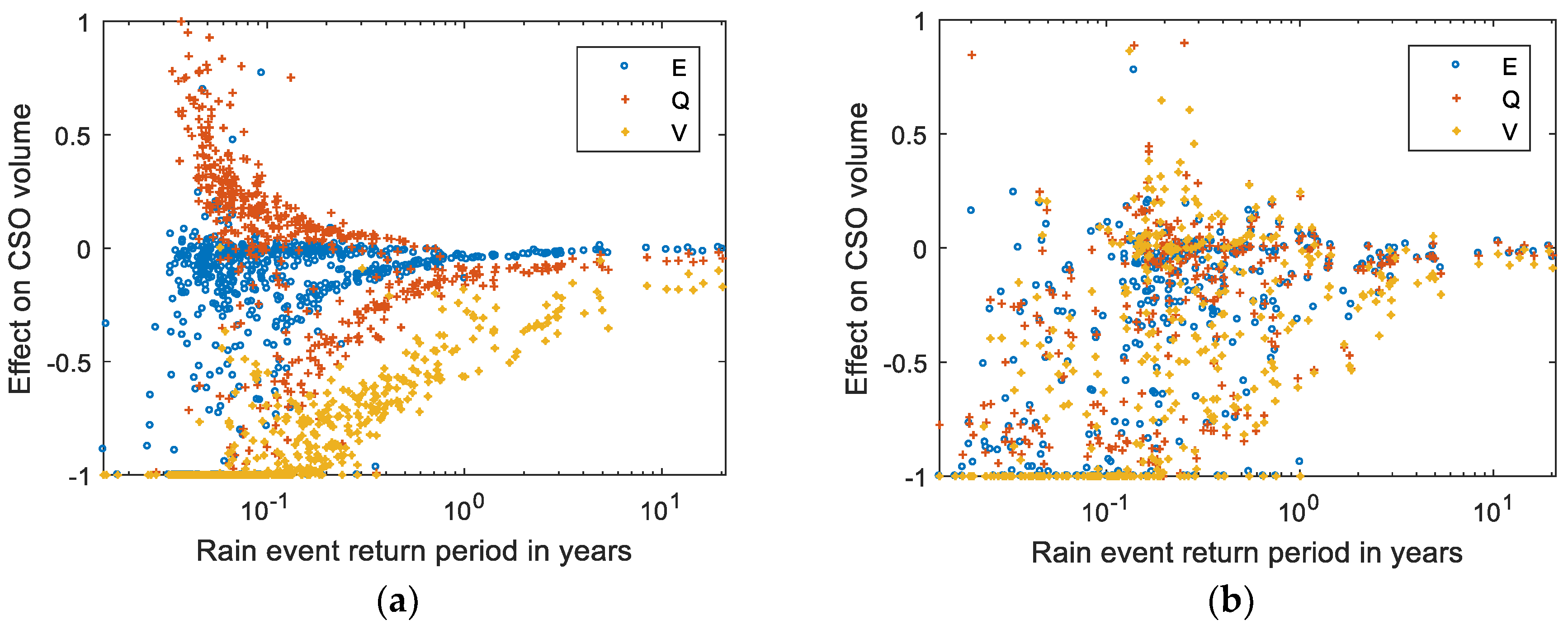
Aside from these findings, the event-based analysis of CSO volumes allows for conclusions on the variability of results, and thus, the viability of the extrapolation of outcomes from the short rain series to general conclusions. For the majority of scenarios run for catchments Beerse and Retie, and for scenarios using existing or a volume-based selection of control locations, the total CSO volume over all events are in close agreement with the mean effect on total CSO volume of single events. For Wolfsdonk and many of the scenarios for Geel, there is an offset, but correlation is high here, too. This is very different for scenarios using flow-based control location selection for catchment Arendonk: The mean effect on CSO volume over all events shows an increase of 12%, but the total effect is reduced by 14%. The reason for this is illustrated by Figure 7a for one control algorithm concept (pid EQ glo). Figure 7b shows an example of expected performance for the same control algorithm applied to catchment Retie for comparison.
For Arendonk, volume-based control location scenarios display a significant reduction of CSO volume for the vast majority of events of any return period, whereas scenarios using existing control locations consistently show little to no effect. The scenario using flow-based control locations shows good CSO volume reduction for events with a medium to high return period, but an increase for a high number of very small events. As the spilled volumes are very small, this can be alleviated by manually tuning the control parameters of the gate without any significant negative influence on the total CSO volume. This example indicates that the scenarios built by the automated routine require thorough investigation by the modeler in order to avoid unnecessary inefficiencies of the applied RTC system.
4. Discussion
The best results for performance improvement by RTC are found for the largest catchment, Geel, with about 50% CSO volume reduction, a good result when comparing to the literature [25]. This is in line with general expectations and the PASST screening [33]. Rather unexpectedly, the smallest catchment with the lowest PASST score still shows a noteworthy reduction in excess of 20%. This discrepancy between the results of the implemented RTC strategies and the PASST screening suggests that, while screening methods such as [16,17] can give a good indication whether or not the implementation of RTC can lead to performance improvements, an exact ranking based on these methods should be avoided.
Overall, both short and long-term simulation results indicate that there is no single ‘best’ control algorithm for the investigated catchments for CSO volume reduction. This is in agreement with the literature discussing one comparable catchment [24]. Results are even very similar between RBC and MPC scenarios. This is in line with previous findings in the literature [58], and indicates that simple control procedures have their place, especially for small networks, alongside more advanced options, and that RBC can be used as viable fallback strategy when implementing more complex MPC, as e.g., suggested by [23]. For larger, more complex catchments, MPC can be expected to outperform RBC [26].
In terms of performance improvement regarding flooding, the added complexity of the more advanced algorithms could be justified for one catchment (Arendonk). While the influence of the chosen algorithm appears limited, the choice of the control locations is of very high importance for system performance, varying between 0 and 50% performance improvement. In four of the five investigated cases, flooding that might be potentially influenced by RTC played an important role. This would have made the use of most conceptual models for such analyses challenging, as the estimation of flood volumes using such models will be difficult, if not unfeasible, especially when controlling in-sewer storage rather than storage basins. This problem could be overcome by the use of conceptual flood models as under recent development [59].
The results of this study show that the automated design of control strategies, i.e., the automated selection of suitable control locations and the design of RBC algorithms, is feasible. For all five tested catchments, the application of the routine leads to useful RTC concepts with considerable performance improvements. The diversity in results obtained for the different catchments showcases that concepts developed for one single case study might lead to highly different results when applied to other systems. While this is not surprising, it still indicates that the use of benchmarking systems as suggested in literature (see e.g., [60,61]), though very desirable, might be very difficult for RTC in sewer systems. Also, while demo projects like [61] and examples as listed by [15] are certainly useful for raising awareness of RTC in general, any project-specific results should be interpreted with great care. The large variety across results of the five investigated catchments suggests that results reported in literature for RTC cannot be extrapolated to other case studies (thus corroborating findings reported e.g., by [57]), and that the usefulness of a control concept for a certain case study can only be assessed by testing. Tool-based procedures for the screening for RTC potential [16,17,18] or RTC strategy implementation with a high degree of automation as the one introduced here can considerably simplify this task, and ultimately help in ‘convincing practitioners’ as requested by other authors (e.g., [32]).
As no single ‘best’ algorithm is found for the here tested catchments, future applications of the procedure will be based on the implementation and evaluation of all available control concepts. This only adds marginal computational burden, as the use of the short rain series as suggested by [62] has proven a very effective means to reduce the simulation duration while still allowing for a ranking of the usefulness of the tested control algorithms. The final performance estimation should, however, still be based on long-term simulations, as the results from short and long-term simulations for the tested cases still show some differences. This is also agreed upon by others [25]. For flooding, the used 1D hydrodynamic models can only give indications, as discrepancies between short and long-term series results show for catchment Arendonk. If flooding is shown to be of high relevance, detailed evaluations should be based on more accurate models calibrated using historical flood events.
As results have shown, automated control location choice forms an important first step when building an RTC strategy after a successful initial screening for RTC potential for operators interested in RTC. The found results suggest that next to the comparison and further improvement of existing control algorithms [23,24], the refinement of the automated selection of control locations applicable for a wide range of case studies could hold high potential for further research and application in urban drainage. Further improvement of the control location choice by including land use as a criterion for the suitability of a location as proposed by [31] could be interesting in the future. This option has not been considered in this study, as the information on land use in the hydrodynamic models used here is not fine-grained enough for such analyses. Rather, the modeler is given the option of choosing control locations manually. This way, it is possible for the modeler to iteratively improve the selection of control locations for optimal results after having run an initial screening using flow- or volume-based control location identification methods.
After all control locations are identified, the methodology designs control algorithms according to generic control concepts, such as global equal filling degree, with default parameters. Although these parameters have been shown to have only limited influence for the here described case study, the results of catchment Retie suggest that performance of other catchments can be sensitive to these parameters. The default parameters should thus always be evaluated for their sensitivity, e.g., by using Morris screening [52], as done here, or by applying other methods [40,54,63]. Influential parameters can be further modified by the modeler until a desirable outcome is reached, either by manually adjusting them in a trial-and-error manner, or based on expert knowledge or through the use of optimization routines [64]. The final parameterization is then to be modified by means of a long-term simulation, ideally using spatially-variable rainfall where available. In any case, the RTC strategies designed by the proposed procedure should always be regarded as a starting point which can be quickly created as a basis for more in-depth analysis of the system.
In order to be able to apply the described procedure for the design of RTC strategies, an existing, detailed and up-to-date hydrodynamic model is used as a starting point. If such a model does not exist, or is too inaccurate with respect to the criteria to be evaluated, application of the procedure should be refrained from. Though the procedure in its current form has been shown to be useful for cases using CSO volume and flooding as evaluated criteria (also used by the majority of RTC related literature [25]), its applicability might be limited to cases where water-quantitative evaluation criteria are used. Though water quality or impact-based control, as recently demonstrated for several case studies [64,65], might be a desirable application, this may require the implementation of a different approach for control location selection.
As all the presently investigated catchments are rather small, and hydraulic complexity is not too high for most of them, the findings of this study should not be expected to hold true for large catchments where continuous improvement of control algorithms has been documented to lead to improved system performance over the years [5,12]. Also, projects that require the formulation of more complex evaluation criteria and control models, as, e.g., for water quality or impact-based control or the explicit consideration of uncertainties in monitoring and prediction [26], complex RBC algorithms or MPC can still be expected to provide advantages over more simplistic control. While MPC allows for equally good results as RBC (this is in line with [1] who used simplified models and [23] who used a detailed model for a larger catchment) for small catchments and straight forward evaluation criteria as investigated here, it is expected that the additional complexity added by MPC will not result in further improvement. While the findings here are expected to give good insight into the potential and applicability of automated design of RTC strategies for existing Flemish urban drainage systems, an even wider scope, allowing for more generic result interpretation, could form a desirable future research topic. The results of such research could play a key role in helping reluctant operators in taking their first steps towards harnessing the potential of RTC for their systems. In Flanders, where many catchments largely resemble the ones used here, the general findings of this study are expected to hold true. The routine described in this paper has been successfully applied to ten further catchments. Detailed modelling and implementation of the resulting RTC scenarios for these catchments is currently under way. Further application of the routine for the design of RTC strategies is planned for five to ten catchments every year.
5. Conclusions
A novel methodology for the automated design of RTC strategies for combined sewer systems has been implemented and tested for five case studies. The following general conclusions can be drawn from this investigation:
- The automated implementation of RTC strategies has led to good results for all five tested case studies.
- No single best control algorithm outperforming other algorithms could be found in terms of CSO volume or flooding.
- Both RBC and MPC are able to lead to considerable CSO volume reduction compared to the uncontrolled scenario.
- In comparison to the achieved system performance, screening methods for the ‘control-worthiness’ of a system can give a good indication whether or not the implementation of RTC can lead to performance improvements for all tested cases; a detailed ranking should, however, be refrained from.
- The selection of control locations plays a major role for the success of an RTC strategy. Scenarios using volume-based control location selection clearly outperform other tested selection strategies.
- Next to control algorithm development, the identification of suitable control locations in sewer systems can constitute a promising research topic in the future.
Author Contributions
Conceptualization, Methodology & Original Draft Preparation: S.K.; Review & Editing: M.W., J.V.I., P.W. All authors have read and approved the final manuscript.
Funding
This research received no external funding.
Acknowledgments
The authors gratefully acknowledge the support from Luca Vezzaro, DTU, for providing the code and documentation of DORA2.
Conflicts of Interest
The authors declare no conflict of interest.
Appendix A
Figure A1 outlines the algorithm for the determination of minimum node drainage levels d used for the identification of overflow locations.
Figure A1.
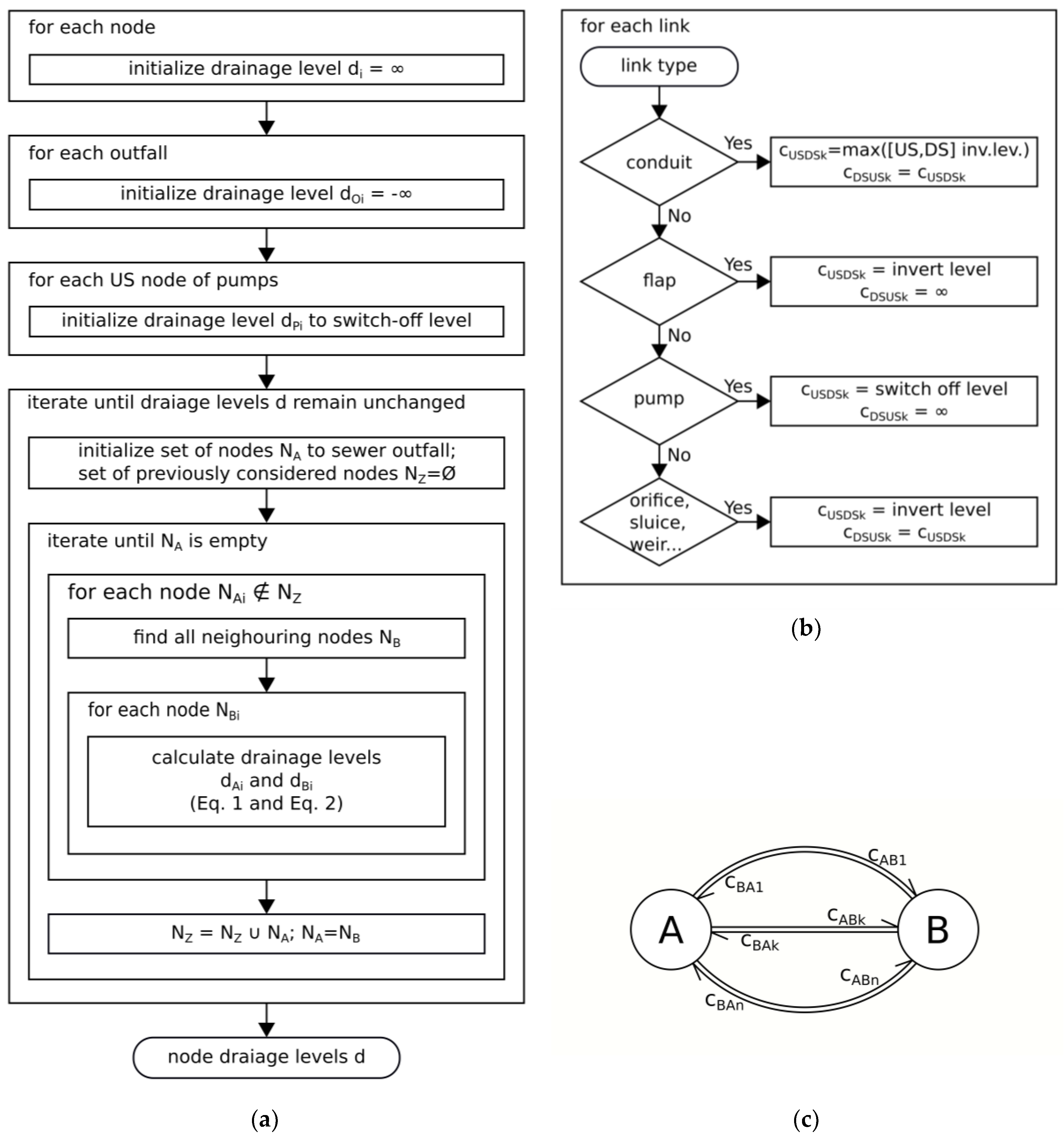
Algorithm for the identification of overflow locations. (a) main algorithm calculating minimum node drainage levels based on constant link data c. (b) determination of constant link invert data c for different link types depending on direction (USDS: from upstream to downstream, DSUS: from downstream to upstream node). (c) Example graph for n links from node A to B (cAB1 to cABn) and from B to A (cBA1 to cBAn).
Figure A1.
Algorithm for the identification of overflow locations. (a) main algorithm calculating minimum node drainage levels based on constant link data c. (b) determination of constant link invert data c for different link types depending on direction (USDS: from upstream to downstream, DSUS: from downstream to upstream node). (c) Example graph for n links from node A to B (cAB1 to cABn) and from B to A (cBA1 to cBAn).

The main algorithm (Figure A1a) iteratively calculates minimum drainage levels d (i.e., the minimum water level required for the water to leave the system via an outfall node) for neighboring nodes applying Equations (A1) and (A2)
for all n links (conduits, flap gates, pumps, orifices, sluices, weirs etc.) connecting the nodes (see Figure A1c). It makes use of the constant invert levels c, which are properties of the links. They are defined by the algorithm shown in Figure A1b. As can be seen, pumps and flap gates are treated depending on their direction, they cannot be passed from downstream (DS) to upstream (US). The node drainage levels are used to assign a hydraulically relevant direction (from US to DS) to each link. These directions can be used for a routing from any node to an outfall. Links with one node draining to the WWTP and another draining to a different outfall are external bifurcations, i.e., overflow locations.
Appendix B
Figure A2.
Morris screening results; (a): mean elementary effect µabs on CSO volume vs subbasin location; (b) mean elementary effect µabs on CSO volume vs subbasin storage capacity; (c): mean elementary effect µabs on CSO volume vs cumulated relative storage capacity; (d) mean elementary effect µabs on CSO volume vs downstream cumulated relative storage capacity.

References
- Broks, K.; Geenen, A.; Nelen, F.; Jacobsen, P. The potential of real time control to reduce combined sewer overflow. Hydrol. Res. 1995, 26, 223–236. [Google Scholar] [CrossRef]
- Campisano, A.; Schilling, W.; Modica, C. Regulators’ setup with application to the Roma–Cecchignola combined sewer system. Urban Water 2000, 2, 235–242. [Google Scholar] [CrossRef]
- Colas, H.; Pleau, M.; Lamarre, J.; Pelletier, G.; Lavallée, P. Practical Perspective on Real-Time Control. Water Qual. Res. J. Can. 2004, 39, 466–478. [Google Scholar] [CrossRef]
- Dirckx, G.; Schütze, M.; Kroll, S.; Thoeye, C.; De Gueldre, G.; Van De Steene, B. Cost-efficiency of RTC for CSO impact mitigation. Urban Water J. 2011, 8, 367–377. [Google Scholar] [CrossRef]
- Pleau, M.; Colas, H.; Lavallee, P.; Pelletier, G.; Bonin, R. Global optimal real-time control of the Quebec urban drainage system. Environ. Model. Softw. 2005, 20, 401–413. [Google Scholar] [CrossRef]
- Vezzaro, L.; Grum, M. A generalised Dynamic Overflow Risk Assessment (DORA) for Real Time Control of urban drainage systems. J. Hydrol. 2014, 515, 292–303. [Google Scholar] [CrossRef] [Green Version]
- Weyand, M. Real time control within a combined sewer system: Comparison of practical and theoretical results. Water Sci. Technol. 1993, 27, 123–132. [Google Scholar] [CrossRef]
- Schilling, W. Association internationale pour la qualité de l’eau. In Real-Time Control of Urban Drainage Systems: The State-of-The Art; IAWPRC; Pergamon Press: London, UK, 1989; ISBN 978-0-08-040145-4. [Google Scholar]
- Schütze, M.; Campisano, A.; Colas, H.; Schilling, W.; Vanrolleghem, P.A. Real-time control of urban wastewater systems–where do we stand today? J. Hydrol. 2004, 299, 335–348. [Google Scholar] [CrossRef]
- Beeneken, T.; Erbe, V.; Messmer, A.; Reder, C.; Rohlfing, R.; Scheer, M.; Schuetze, M.; Schumacher, B.; Weilandt, M.; Weyand, M. Real time control (RTC) of urban drainage systems—A discussion of the additional efforts compared to conventionally operated systems. Urban Water J. 2013, 10, 293–299. [Google Scholar] [CrossRef]
- Fuchs, L.; Beeneken, T. Development and implementation of a real-time control strategy for the sewer system of the city of Vienna. Water Sci. Technol. 2005, 52, 187–194. [Google Scholar] [CrossRef] [PubMed]
- Günther, H.; Lindenberg, M. Konzeption einer Abflusssteuerung am Beispiel Dresden. Innov. Abwasserableitung Abwassersteuerung 2002, 21, 303–324. [Google Scholar]
- Rohlfing, R.; Wiemann, M. Optimierte Dimensionierung und Bewirtschaftung von Kläranlagen- und Kanalkapazitäten bei Berücksichtigung der Echtzeitsteuerung—Beispiel Leipzig. Innov. Abwasserableitung Abwassersteuerung 2002, 21, 75–85. [Google Scholar]
- Seggelke, K.; Löwe, R.; Beeneken, T.; Fuchs, L. Implementation of an integrated real-time control system of sewer system and waste water treatment plant in the city of Wilhelmshaven. Urban Water J. 2013, 10, 330–341. [Google Scholar] [CrossRef]
- Erbe, V. Kanalnetzsteuerung-Überblick über umgesetzte Projekte und Erfahrungen aus der Praxis. Innov. Abwasserableitung Abwassersteuerung 2002, 21, 35–51. [Google Scholar]
- Schütze, M.; Erbe, V.; Haas, U.; Scheer, M.; Weyand, M. PASST—A planning aid for sewer system real time control. In Proceedings of the 6th International Conference on Urban Drainage Modelling, Dresden, Germany, 15–17 September 2004. [Google Scholar]
- Zacharof, A.I.; Butler, D.; Schütze, M.; Beck, M.B. Screening for real-time control potential of urban wastewater systems. J. Hydrol. 2004, 299, 349–362. [Google Scholar] [CrossRef]
- Framework for Planning of Real Time Control of Sewer Networks, DWA ed.; German DWA Rules and Standards Advisory Leaflet; December 2005; DWA: Hennef, Germany, 2008; ISBN 978-3-939057-28-4.
- Messmer, A.; Schütze, M.; Ogurek, M. A demonstration software tool for real time control of urban drainage systems. In Proceedings of the 11th International Conference on Urban Drainage (ICUD), Edinburgh, UK, 31 August–5 September 2008. [Google Scholar]
- Borsányi, P.; Benedetti, L.; Dirckx, G.; De Keyser, W.; Muschalla, D.; Solvi, A.-M.; Vandenberghe, V.; Weyand, M.; Vanrolleghem, P.A. Modelling real-time control options on virtual sewer systems. J. Environ. Eng. Sci. 2008, 7, 395–410. [Google Scholar] [CrossRef]
- Alex, J.; Schütze, M.; Ogurek, M.; Jumar, U. Systematic Design of Distributed Controllers for Sewer Networks. In Proceedings of the 17th World Congress the International Federation of Automatic Control, Seoul, Korea, 6–11 July 2008; pp. 556–561. [Google Scholar]
- Kroll, S.; Weemaes, M.; Van Impe, J.; Willems, P. A generic concept for storage control in sewer systems. In Proceedings of the 14th International Conference on Urban Drainage, Prague, Czech Republic, 10–15 September 2017. [Google Scholar]
- Meneses, E.J.; Gaussens, M.; Jakobsen, C.; Mikkelsen, P.S.; Grum, M.; Vezzaro, L. Coordinating Rule-Based and System-Wide Model Predictive Control Strategies to Reduce Storage Expansion of Combined Urban Drainage Systems: The Case Study of Lundtofte, Denmark. Water 2018, 10, 76. [Google Scholar] [CrossRef]
- Klepiszewski, K.; Schmitt, T.G. Comparison of conventional rule based flow control with control processes based on fuzzy logic in a combined sewer system. Water Sci. Technol. 2002, 46, 77–84. [Google Scholar] [CrossRef] [PubMed]
- Lund, N.S.V.; Falk, A.K.V.; Borup, M.; Madsen, H.; Mikkelsen, P.S. Model predictive control of urban drainage systems: A review and perspective towards smart real-time water management. Crit. Rev. Environ. Sci. Technol. 2018, 48, 279–339. [Google Scholar] [CrossRef] [Green Version]
- Löwe, R.; Vezzaro, L.; Mikkelsen, P.S.; Grum, M.; Madsen, H. Probabilistic runoff volume forecasting in risk-based optimization for RTC of urban drainage systems. Environ. Model. Softw. 2016, 80, 143–158. [Google Scholar] [CrossRef] [Green Version]
- Leitão, J.P.; Carbajal, J.P.; Rieckermann, J.; Simões, N.E.; Sá Marques, A.; de Sousa, L.M. Identifying the best locations to install flow control devices in sewer networks to enable in-sewer storage. J. Hydrol. 2018, 556, 371–383. [Google Scholar] [CrossRef]
- Philippon, V.; Riechel, M.; Stapf, M.; Sonnenberg, H.; Schütze, M.; Pawlowsky-Reusing, E.; Rouault, P. How to find suitable locations for in-sewer storage? Test on a combined sewer catchment in Berlin. In Proceedings of the 10th International Urban Drainage Modelling Conference, Beaupré, QC, Canada, 20–23 September 2015; Volume 1, pp. 295–298. [Google Scholar]
- Kroll, S.; Wambecq, T.; Weemaes, M.; Van Impe, J.; Willems, P. Semi-automated buildup and calibration of conceptual sewer models. Environ. Model. Softw. 2017, 93, 344–355. [Google Scholar] [CrossRef]
- Van Daal, P.; Gruber, G.; Langeveld, J.; Muschalla, D.; Clemens, F. Performance evaluation of real time control in urban wastewater systems in practice: Review and perspective. Environ. Model. Softw. 2017, 95, 90–101. [Google Scholar] [CrossRef]
- Van daal-Rombouts, P.; Sun, S.; Langeveld, J.; Bertrand-Krajewski, J.-L.; Clemens, F. Design and performance evaluation of a simplified dynamic model for combined sewer overflows in pumped sewer systems. J. Hydrol. 2016, 538, 609–624. [Google Scholar] [CrossRef] [Green Version]
- Cembrano, G. Keynote: Blue water, green and grey infrastructure—Why control theory matters. In Proceedings of the 14th International Conference on Urban Drainage, Prague, Czech Republic, 10–15 September 2017. [Google Scholar]
- Dirckx, G.; Thoeye, C.; De Gueldre, G.; Van De Steene, B. PASST een RTC strategie in Vlaanderen? Rioleringswetenschap 2007, 7, 38–52. [Google Scholar]
- Innovyze Ltd. InfoWorks Integrated Catchment Modeling (ICM); Innovyze Ltd.: Wallingford, UK, 2016. [Google Scholar]
- Aquafin. Hydronaut Procedure Versie 7.0; Aquafin: Aartselaar, Belgium, 2017. [Google Scholar]
- Mathworks. Matlab; The MathWorks, Inc.: Natick, MA, USA, 2017. [Google Scholar]
- Vonach, T.; Tscheikner-Gratl, F.; Rauch, W.; Kleidorfer, M. A Heuristic Method for Measurement Site Selection in Sewer Systems. Water 2018, 10, 122. [Google Scholar] [CrossRef]
- Meijer, D.; van Bijnen, M.; Langeveld, J.; Korving, H.; Post, J.; Clemens, F. Identifying Critical Elements in Sewer Networks Using Graph-Theory. Water 2018, 10, 136. [Google Scholar] [CrossRef]
- Ermolin, Y.A. Mathematical modelling for optimized control of Moscow’s sewer network. Appl. Math. Model. 1999, 23, 543–556. [Google Scholar] [CrossRef]
- Kroll, S.; Dirckx, G.; Donckels, B.M.R.; Van Dorpe, M.; Weemaes, M.; Willems, P. Modelling real-time control of WWTP influent flow under data scarcity. Water Sci. Technol. 2016, 73, 1637–1643. [Google Scholar] [CrossRef] [PubMed]
- Carstensen, J.; Nielsen, M.; Harremoes, P. Predictive control of sewer systems by means of grey-box models. Water Sci. Technol. 1996, 34, 189–194. [Google Scholar] [CrossRef]
- Ostojin, S.; Mounce, S.R.; Boxall, J.B. An artificial intelligence approach for optimizing pumping in sewer systems. J. Hydroinform. 2011, 13, 295–306. [Google Scholar] [CrossRef] [Green Version]
- Fiorelli, D.; Schutz, G.; Klepiszewski, K.; Regneri, M.; Seiffert, S. Optimised real time operation of a sewer network using a multi-goal objective function. Urban Water J. 2013, 10, 342–353. [Google Scholar] [CrossRef]
- Regneri, M. Modeling and Multi-Objective Optimal Control of integrated Wastewater Collection and Treatment Systems in Rural Areas Based on Fuzzy Decision-Making; Schriftenreihe zur Wasserwirtschaft; Technische Universität Graz: Graz, Austria, 2015; ISBN 978-3-85125-381-8. [Google Scholar]
- Erbe, V.; Risholt, L.; Schilling, W.; Londong, J. Integrated modelling for analysis and optimisation of wastewater systems–the Odenthal case. Urban Water 2002, 4, 63–71. [Google Scholar] [CrossRef]
- Cembrano, G.; Quevedo, J.; Salamero, M.; Puig, V.; Figueras, J.; Martí, J. Optimal control of urban drainage systems. A case study. Control Eng. Pract. 2004, 12, 1–9. [Google Scholar] [CrossRef] [Green Version]
- Männing, F. Abflusssteuerung des Dresdner Mischwassernetzes. Wasser Abfall 2006, 8, 10–15. [Google Scholar]
- Einfalt, T.; Stölting, B. Real-Time Control for Two Communities—Technical and Administrational Aspects. In Proceedings of the Ninth International Conference on Urban Drainage, Portland, OR, USA, 8–13 September 2002; pp. 320–331. [Google Scholar]
- Rossman, L.A. Storm Water Management Model: User’s Manual, Version 5.0; United States Environmental Protection Agency: Cincinnati, OH, USA, 2005.
- Riaño-Briceño, G.; Barreiro-Gomez, J.; Ramirez-Jaime, A.; Quijano, N.; Ocampo-Martinez, C. MatSWMM–An open-source toolbox for designing real-time control of urban drainage systems. Environ. Model. Softw. 2016, 83, 143–154. [Google Scholar] [CrossRef]
- Riaño-Briceño, G.A. MatSWMM 5.1.012. Networked Systems, 2017. Available online: https://github.com/networked-systems/MatSWMM (accessed on 4 July 2018).
- Morris, M.D. Factorial Sampling Plans for Preliminary Computational Experiments. Technometrics 1991, 33, 161–174. [Google Scholar] [CrossRef] [Green Version]
- Campolongo, F.; Cariboni, J.; Saltelli, A. An effective screening design for sensitivity analysis of large models. Environ. Model. Softw. 2007, 22, 1509–1518. [Google Scholar] [CrossRef]
- Vanrolleghem, P.A.; Mannina, G.; Cosenza, A.; Neumann, M.B. Global sensitivity analysis for urban water quality modelling: Terminology, convergence and comparison of different methods. J. Hydrol. 2015, 522, 339–352. [Google Scholar] [CrossRef] [Green Version]
- Sriwastava, A.K.; Tait, S.; Schellart, A.; Kroll, S.; Dorpe, M.V.; Assel, J.V.; Shucksmith, J. Quantifying Uncertainty in Simulation of Sewer Overflow Volume. J. Environ. Eng. 2018, 144, 04018050. [Google Scholar] [CrossRef]
- Waterinfo.be. WATERINFO.be—Download. Available online: https://www.waterinfo.be/default.aspx?path=NL/Rapporten/Downloaden (accessed on 18 February 2018).
- Schütze, M.; Erbe, V.; Haas, U.; Scheer, M.; Weyand, M. Sewer system real-time control supported by the M180 guideline document. Urban Water J. 2008, 5, 69–78. [Google Scholar] [CrossRef]
- Mollerup, A.L.; Mikkelsen, P.S.; Sin, G. A methodological approach to the design of optimising control strategies for sewer systems. Environ. Model. Softw. 2016, 83, 103–115. [Google Scholar] [CrossRef] [Green Version]
- Bermúdez, M.; Ntegeka, V.; Wolfs, V.; Willems, P. Development and Comparison of Two Fast Surrogate Models for Urban Pluvial Flood Simulations. Water Resour. Manag. 2018, 32, 2801–2815. [Google Scholar] [CrossRef]
- Saagi, R. Benchmark Simulation Model for Integrated Urban Wastewater Systems-Model Development and Control Strategy Evaluation; Lund University: Lund, Sweden, 2017. [Google Scholar]
- Schütze, M.; Lange, M.; Pabst, M.; Haas, U. Astlingen—A benchmark for real time control (RTC). Water Sci. Technol. 2018, 2017, 552–560. [Google Scholar] [CrossRef] [PubMed]
- Leimgruber, J.; Steffelbauer, D.; Kaschutnig, M.; Tscheikner-Gratl, F.; Muschalla, D. Optimized series of rainfall events for model based assessment of combined sewer systems. In Proceedings of the 9th International Conference NOVATECH 2016, Lyon, France, 28 June–1 July 2016; p. 6. [Google Scholar]
- Gamerith, V.; Neumann, M.B.; Muschalla, D. Applying global sensitivity analysis to the modelling of flow and water quality in sewers. Water Res. 2013, 47, 4600–4611. [Google Scholar] [CrossRef] [PubMed]
- Meng, F.; Fu, G.; Butler, D. Cost-Effective River Water Quality Management using Integrated Real-Time Control Technology. Environ. Sci. Technol. 2017, 51, 9876–9886. [Google Scholar] [CrossRef] [PubMed]
- Langeveld, J.G.; Benedetti, L.; de Klein, J.J.M.; Nopens, I.; Amerlinck, Y.; van Nieuwenhuijzen, A.; Flameling, T.; van Zanten, O.; Weijers, S. Impact-based integrated real-time control for improvement of the Dommel River water quality. Urban Water J. 2013, 10, 312–329. [Google Scholar] [CrossRef]
Figure 1.
Identification of overflow locations.

Figure 2.
Identification of potential control locations: (a) based on flow capacity (case 1, 2: potential control location, case 3: no control location); (b) based on activated storage volume; dark blue: potentially activated storage volume.
Figure 2.
Identification of potential control locations: (a) based on flow capacity (case 1, 2: potential control location, case 3: no control location); (b) based on activated storage volume; dark blue: potentially activated storage volume.

Figure 3.
Storage activation potential by different selection strategies for control locations (E: existing locations, Q: flow-based, V: volume-based). (a) Controlled volumes and number of control locations; (b) distribution of controlled volume per control location.
Figure 3.
Storage activation potential by different selection strategies for control locations (E: existing locations, Q: flow-based, V: volume-based). (a) Controlled volumes and number of control locations; (b) distribution of controlled volume per control location.

Figure 4.
Morris screening results: Effect of parameter variation on total CSO volume and total flood volume with respect to the uncontrolled system for 24 chosen events for all control scenarios and control location identification procedures for Arendonk (a,b), Beerse (c,d), Geel (e,f), Retie (g,h) and Wolfsdonk (i, j). ♢: initial scenario with default parameterization.


Figure 5.
Morris screening results; (a): mean absolute elementary effect µabs on CSO volume per control algorithm parameter, for all control locations of all catchments; (b) mean absolute elementary effect µabs on CSO volume vs relative downstream basin volume for all control locations of all catchments.

Figure 6.
Effect on total CSO volume and total flood volume with respect to the uncontrolled system per event for all events of the 13-year rainfall series for all control scenarios and control location identification procedures for Arendonk (a,b), Beerse (c,d), Geel (e,f), Retie (g,h), and Wolfsdonk (i,j).


Figure 7.
Comparison of the effect on CSO volume per rain event for existing (E), flow- (Q) and volume- (V) based control selection choice; catchments Arendonk (a) and Retie (b); control algorithm: proportionally controlled global equal filling degree (pid EQ glo).
Figure 7.
Comparison of the effect on CSO volume per rain event for existing (E), flow- (Q) and volume- (V) based control selection choice; catchments Arendonk (a) and Retie (b); control algorithm: proportionally controlled global equal filling degree (pid EQ glo).


Table 1.
Summary of characteristics of the selected case studies.
| Arendonk | Beerse | Geel | Retie | Wolfsdonk | |
|---|---|---|---|---|---|
| Total contributing area in ha | 479 | 650 | 1227 | 618 | 877 |
| Reduced contributing area in ha | 113 | 139 | 251 | 64 | 25 |
| Population equivalents | 15,100 | 12,780 | 20,080 | 5380 | 4210 |
| Total pipe length in km | 69.8 | 106.6 | 156.2 | 74.9 | 66.9 |
| Number of nodes | 1513 | 1386 | 1428 | 708 | 570 |
| Number of PS 1 | 7 | 12 | 13 2 | 8 | 13 |
| RTC potential based on [33] | Medium | High | Very high | Medium | Low |
1 including WWTP influent works; 2 two hydraulically independent influent works at the WWTP.
Table 2.
Evaluated control algorithm concepts.
| Short Name | Control Algorithm Description |
|---|---|
| pos DS loc | 2-point-controlled actuator based on local downstream filling degree |
| pos DS glo | 2-point-controlled actuator based on global downstream filling degree |
| pos EQ glo | 2-point-controlled actuator based on global equal filling degree [4] |
| pid DS loc | Proportionally controlled actuator based on local downstream filling degree |
| pid DS glo | Proportionally controlled actuator based on global downstream filling degree |
| pid EQ glo | Proportionally controlled actuator based on global equal filling degree |
| cs DS loc | Capacity splitting controlled actuator based on local downstream filling degree [22] |
| qw DS loc | Qwish-negotiated actuator control based on local downstream filling degree [21] |
| MPC | Model predictive control optimizing for minimization of total CSO volume using DORA2 [6]; model Arendonk only |
Table 3.
Parameter ranges for RTC parameters, depending on setpoint tracking scenario.
| Setpoint Tracking Scenario | Parameter Name | Default Value | Lower Boundary | Upper Boundary | Parameter Description |
|---|---|---|---|---|---|
| pos | FDmax | 1 | 0.90 | 1.05 | Filling degree at which 100% filling of the subbasin is assumed (CSO becomes active) |
| pid | FDmax | 1 | 0.90 | 1.05 | See above |
| p | 1 | 0.5 | 1.5 | Proportional gain of the PID controller for local setpoint tracking of sluices | |
| cs | FDmax | 0.95 | 0.90 | 1.05 | See above |
| T | 300 s | 60 s | 500 s | Period over which the downstream subbasin may be filled up to its setpoint (see [22]) | |
| qw | FDmax | 0.95 | 0.90 | 1.05 | See above |
| T | 300 s | 60 s | 500 s | See above | |
| Qmin 1 | Max. DWF | −100% | +100% | Minimum allowed flow capacity of the control location (see [21]) |
1: Boundaries relative to default value.
Table 4.
Parameter ranges relative to the default value for network parameters of the uncontrolled scenario.
Table 4.
Parameter ranges relative to the default value for network parameters of the uncontrolled scenario.
| Parameter Name | Default Value | Lower Boundary | Upper Boundary |
|---|---|---|---|
| Runoff coefficient | 0.8 | −10% | +10% |
| CSO crest level | Measured value | −10 cm | +10 cm |
| Weir discharge coefficient | 0.66 | −20% | +20% |
Table 5.
Number of control locations and resulting total volume that can be controlled by the application of different control location identification algorithms (E: existing; Q: flow-based; V: volume-based).
Table 5.
Number of control locations and resulting total volume that can be controlled by the application of different control location identification algorithms (E: existing; Q: flow-based; V: volume-based).
| Number of Control Locations | Total Controlled Volume in m³ | |||||
|---|---|---|---|---|---|---|
| Control Location Scenario | E | Q | V | E | Q | V |
| Arendonk | 9 | 14 | 17 | 6163 | 10,261 | 12,278 |
| Beerse | 17 | 18 | 20 | 6125 | 6190 | 9920 |
| Geel | 16 | 23 | 24 | 9920 | 29,362 | 35,115 |
| Retie | 12 | 13 | 15 | 5116 | 5766 | 8487 |
| Wolfsdonk | 14 | 15 | 13 | 8194 | 8122 | 8162 |
© 2018 by the authors. Licensee MDPI, Basel, Switzerland. This article is an open access article distributed under the terms and conditions of the Creative Commons Attribution (CC BY) license (http://creativecommons.org/licenses/by/4.0/).
Share and Cite
MDPI and ACS Style
Kroll, S.; Weemaes, M.; Van Impe, J.; Willems, P. A Methodology for the Design of RTC Strategies for Combined Sewer Networks. Water 2018, 10, 1675. https://doi.org/10.3390/w10111675
AMA Style
Kroll S, Weemaes M, Van Impe J, Willems P. A Methodology for the Design of RTC Strategies for Combined Sewer Networks. Water. 2018; 10(11):1675. https://doi.org/10.3390/w10111675
Chicago/Turabian StyleKroll, Stefan, Marjoleine Weemaes, Jan Van Impe, and Patrick Willems. 2018. "A Methodology for the Design of RTC Strategies for Combined Sewer Networks" Water 10, no. 11: 1675. https://doi.org/10.3390/w10111675
Note that from the first issue of 2016, this journal uses article numbers instead of page numbers. See further details here.