Automated Geospatial Models of Varying Complexities for Pine Forest Evapotranspiration Estimation with Advanced Data Mining


Abstract
:1. Introduction
- Artificial neural networks (ANN) models using Landsat based digital information with back-propagation neural network (BPNN) and radial basis function network (RBFN) algorithms to predict homogenous pine forest daily (noon–2 PM average) ET flux on pixel- or plot average- scale;
- An automated geospatial tool supported by the remotely sensed digital information and ET flux statistical correlation algorithm to help land managers to map pine spatially distributed daily (noon–2 PM average) ET rates in ArcGIS software; and
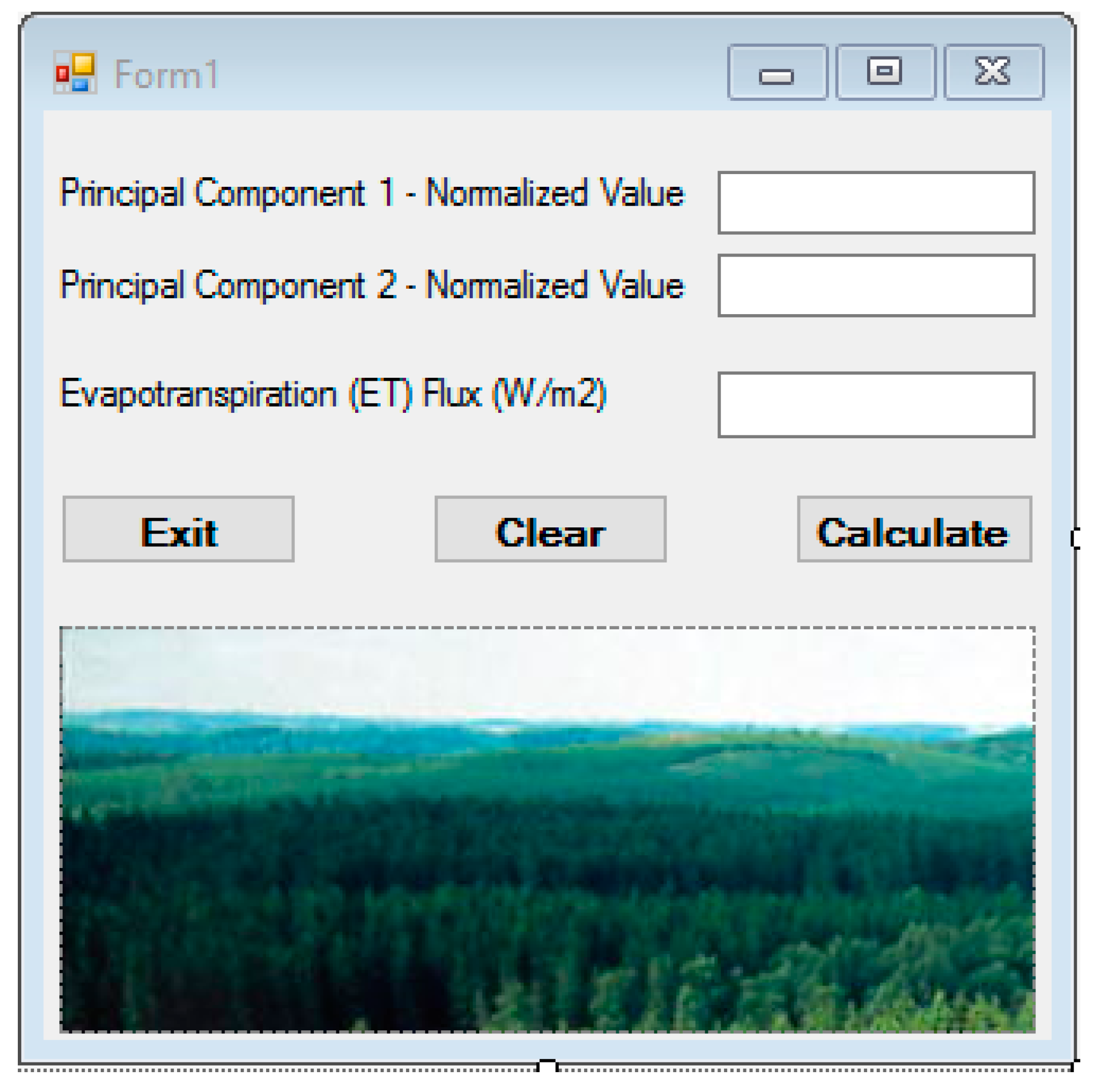
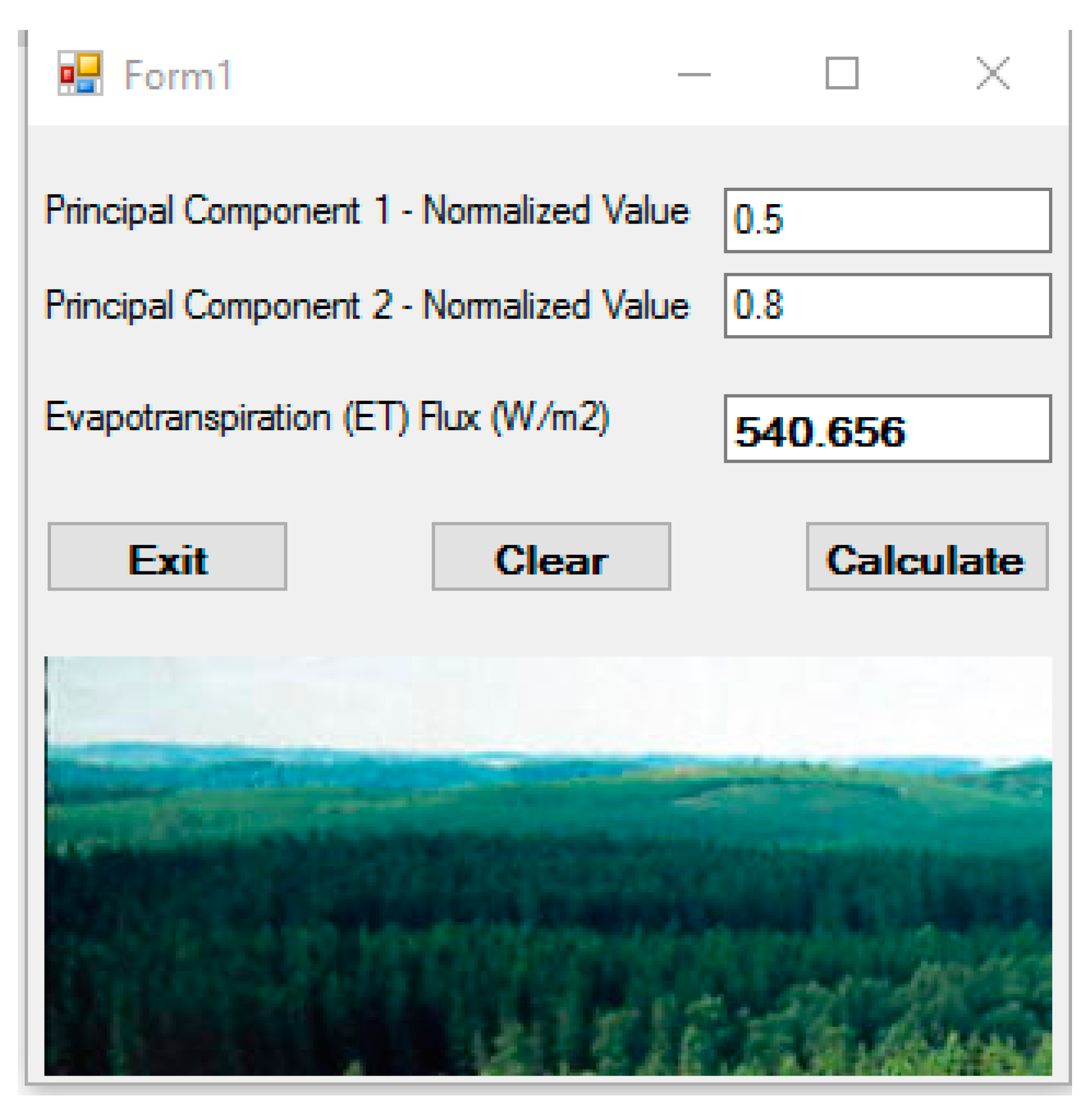
- Executable software that estimates daily (noon–2 PM average) ET rates of homogenous pine forest on pixel- or plot average- scale with the PC bands 1 and 2 information.
2. Methodology
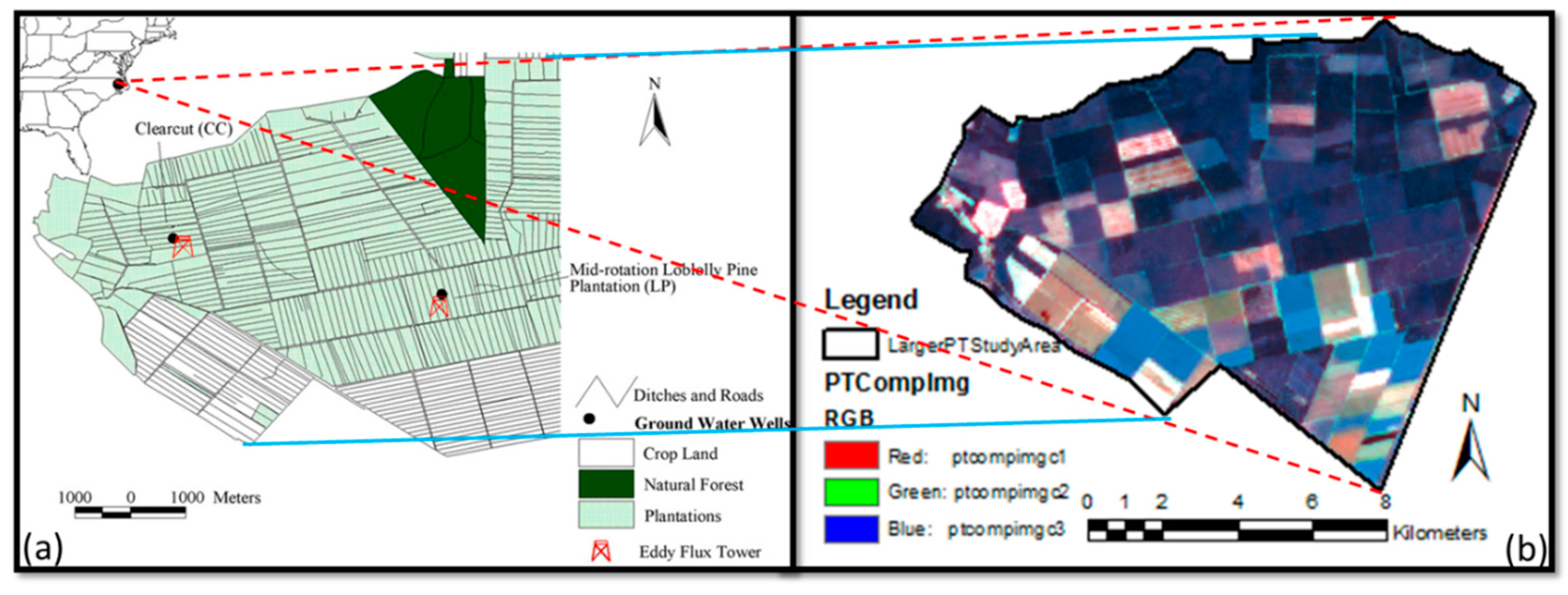
2.1. Study Site
2.2. Data Acquisition
2.2.1. Micrometeorological Data Acquisition and Preparation
2.2.2. Satellite Image Acquisition and Band Selection
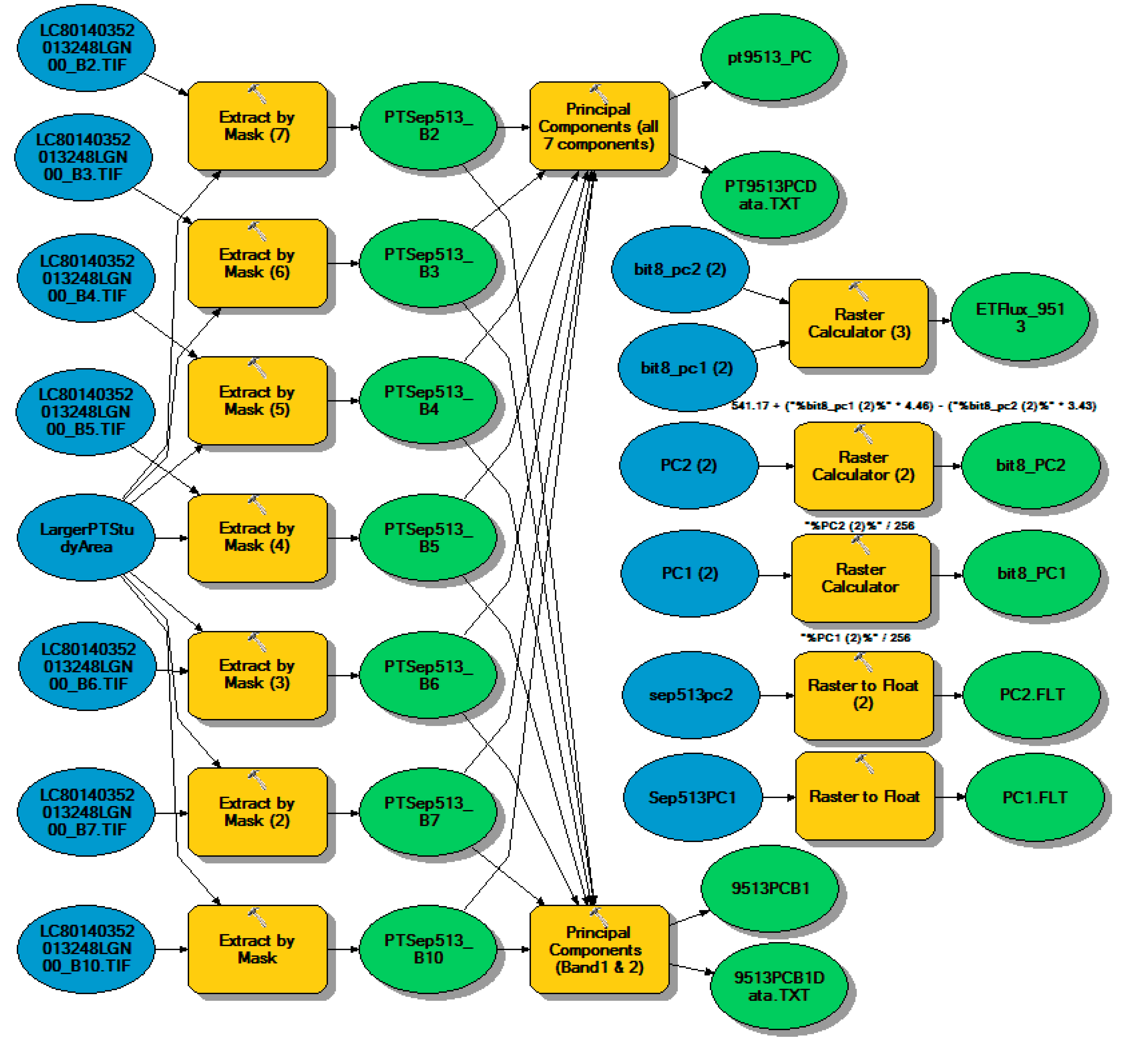
2.2.3. Reduction of Spectral Variables through Principal Components Analysis
2.3. Data Mining Approaches for Model Data Preparation
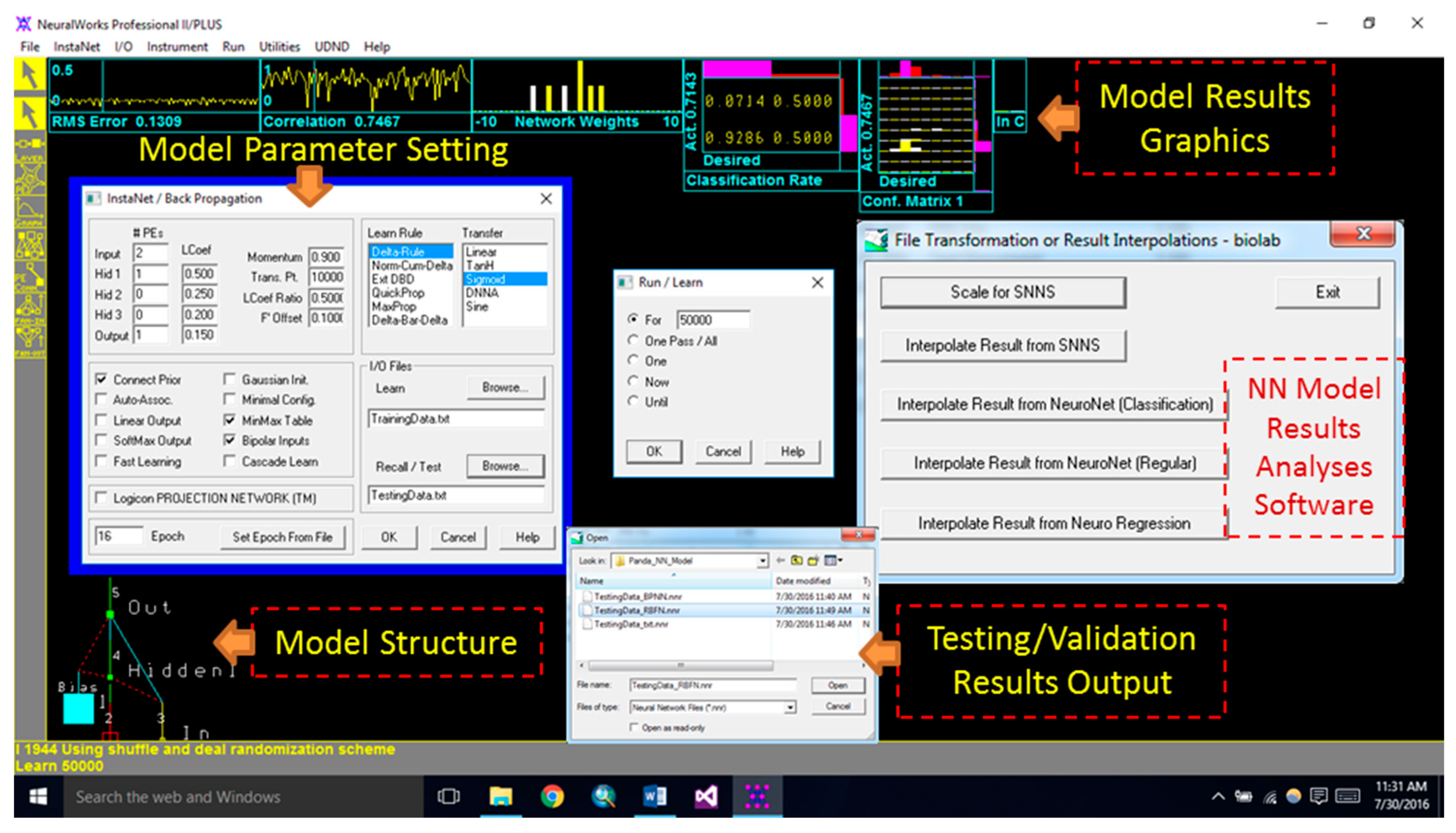
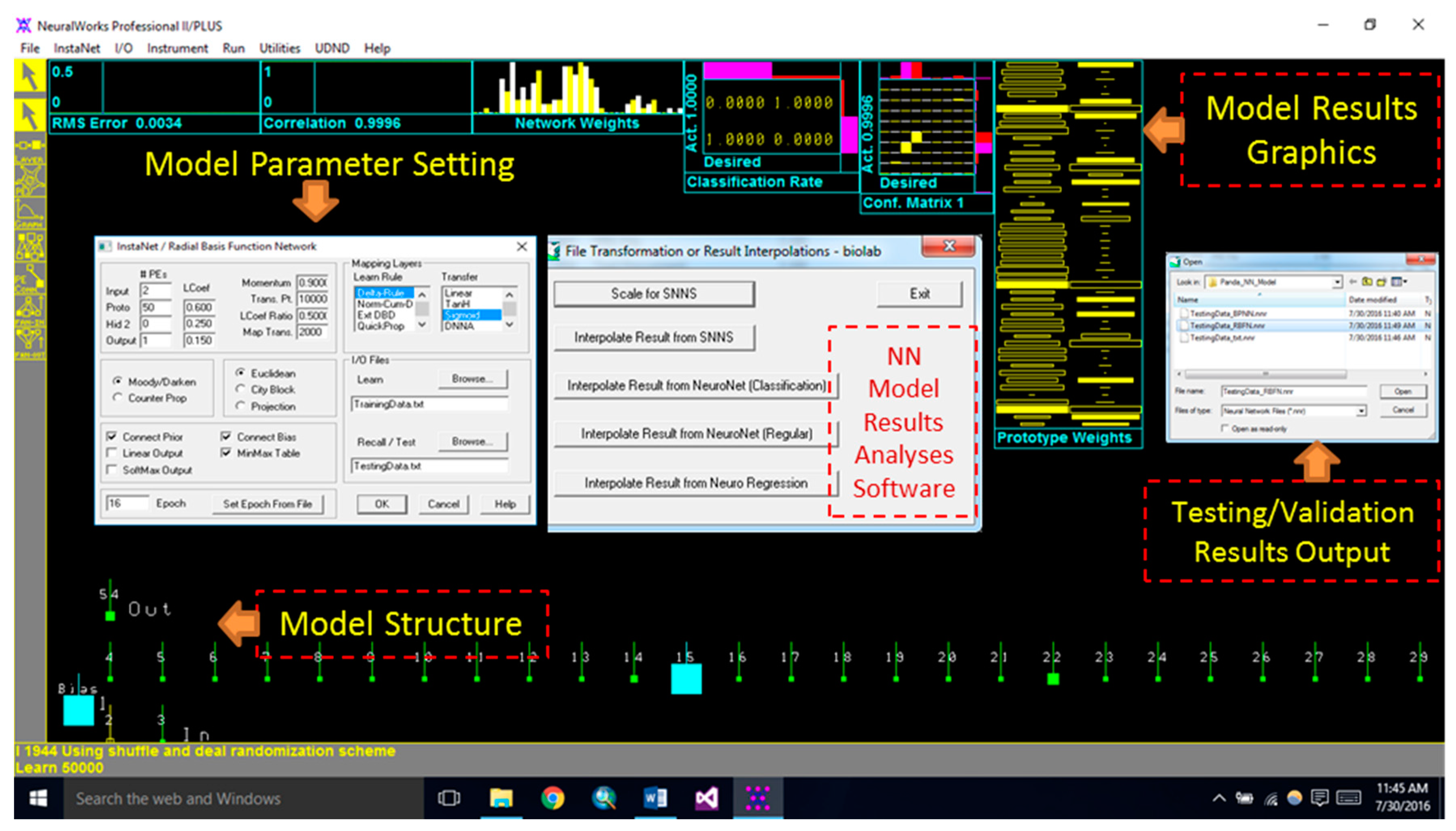
2.4. Neural Network Model Development
Neural Network Model Performance Evaluation
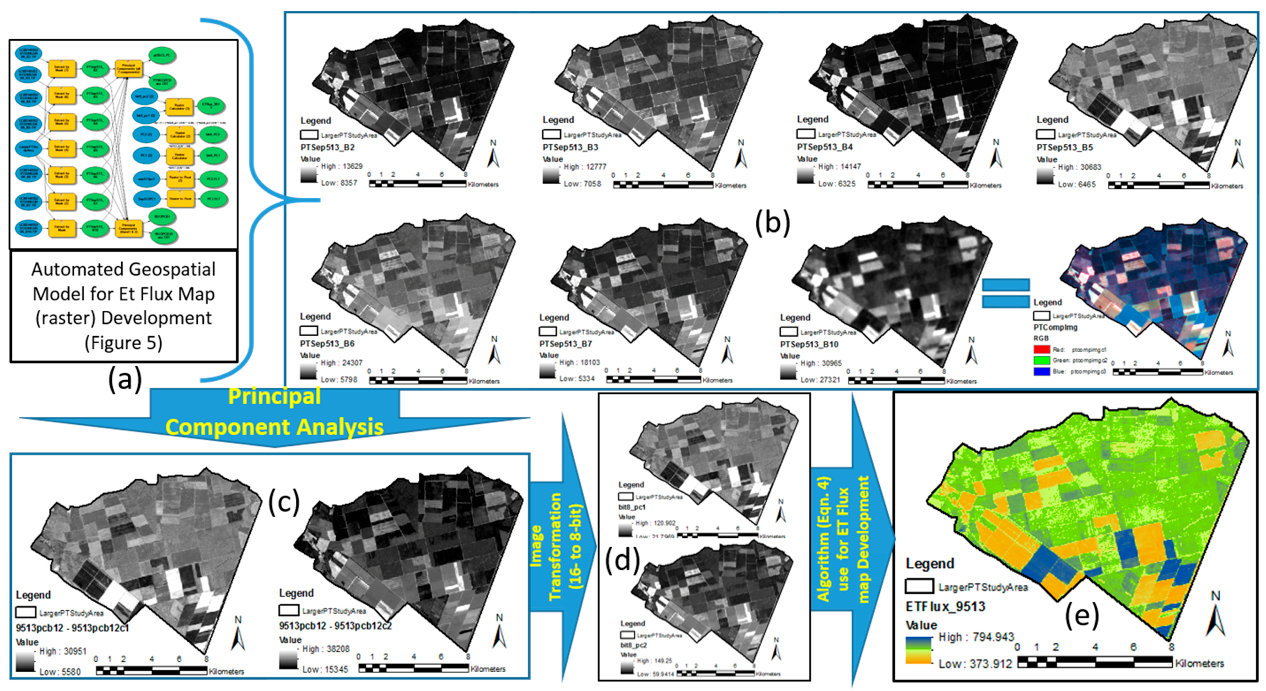
2.5. Automated Geospatial Model and Software Development for ET Estimation
2.5.1. Correlation Algorithm Development and Software Development for ET Prediction
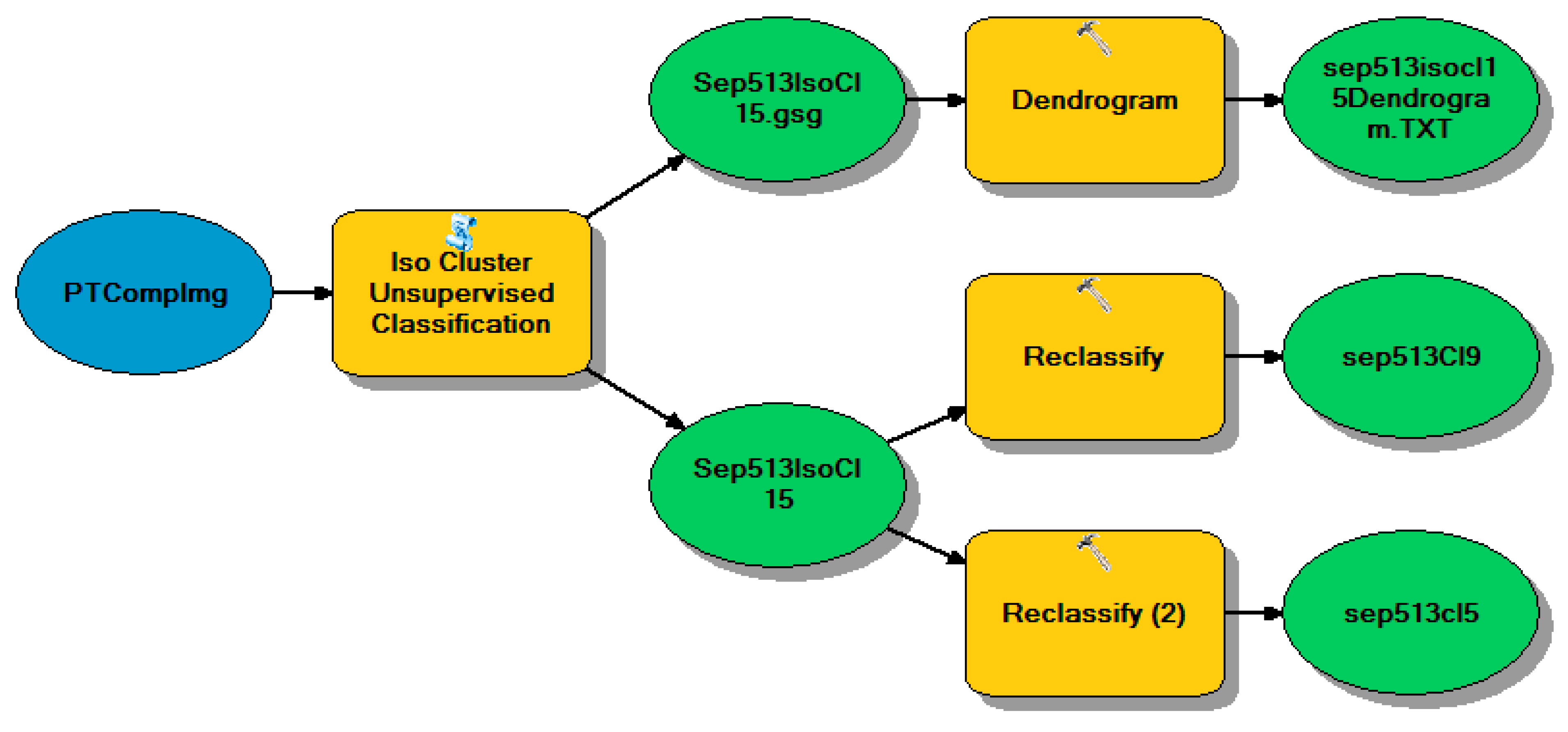
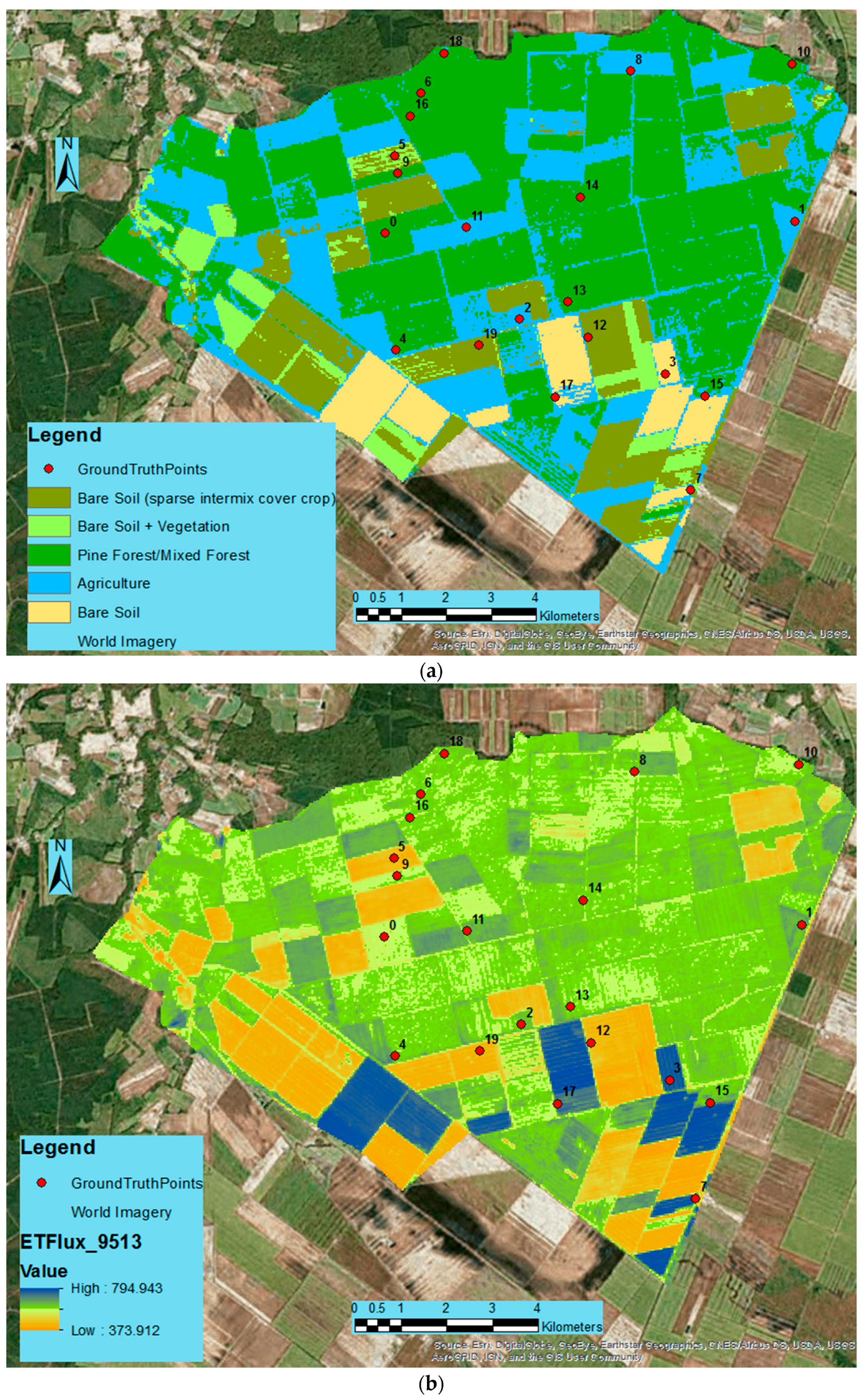
2.5.2. Automated Geospatial Model Development for ET Estimation Map Production
2.5.3. Study Result Validation
3. Results and Discussion
3.1. ET Prediction Model Results
3.1.1. BPNN Training and Validation Models
3.1.2. RBFN Training and Validation Models
3.1.3. Software Development for ET Prediction
3.1.4. ET Flux Map Comparison with Other Studies
3.1.5. Uncertainty and Limitations
4. Summary and Conclusions
Author Contributions
Funding
Acknowledgments
Conflicts of Interest
Appendix A
Appendix A.1. Python Script for PCA Batch Scripting (Partially Shown in Figure Above)

Appendix A.2. Principal Component Analysis Model Development to Automate the Process in Model Input Parameters Creation

Appendix B. ET Flux Estimation Software Developed in Visual Basics Studio


Codes:

Public Class Form1

Private Sub Button3_Click(sender As Object, e As EventArgs) Handles Button3.Click
Me.Close()
End Sub

Private Sub Button2_Click(sender As Object, e As EventArgs) Handles Button2.Click
decPC1.Text = String.Empty
decPC2.Text = String.Empty
txtETFlux.Text = String.Empty
End Sub

Private Sub Button1_Click(sender As Object, e As EventArgs) Handles Button1.Click
Dim decimalPC1 As Decimal ‘Landsat imagery Principal Component Band 1 value
Dim decimalPC2 As Decimal ‘Landsat imagery Principal Component Band 2 value
Dim decimalETFlux As Decimal ‘ET Flux (w/m2) value as result

decimalPC1 = CDec(decPC1.Text)
decimalPC2 = CDec(decPC2.Text)

‘Calculate the ET Flux (W/m2) using the following algorithm
decimalETFlux = 541.17 + (decimalPC1 * 4.46) - (decimalPC2 * 3.43)
txtETFlux.Text = decimalETFlux.ToString
End Sub
        End Class
Appendix C. BPNN Testing Model Prediction Result

| Actual0 | Predicted0 | Absolute Error0 | Accuracy0 |
|---|---|---|---|
| 0.875407 | 0.582837 | 0.29257 | 66.579 |
| 0.520206 | 0.462012 | 0.058194 | 88.8133 |
| 0.676164 | 0.585652 | 0.090512 | 86.6139 |
| 0.943428 | 0.712031 | 0.231397 | 75.4727 |
| 0.668164 | 0.579851 | 0.088313 | 86.6345 |
| 1.42101 | 1.54351 | 0.12250 | 91.3323 |
| 1.12945 | 0.945626 | 0.18382 | 83.7248 |
| 1.41502 | 1.53342 | 0.118395 | 91.633 |
| 1.32868 | 1.64654 | 0.317865 | 76.0766 |
Appendix D. RBFN Testing Model Prediction Result
| Actual0 | Predicted0 | Absolute Error0 | Accuracy0 |
|---|---|---|---|
| 0.875407 | 0.806028 | 0.069379 | 92.0747 |
| 0.520206 | 0.605002 | 0.084796 | 83.6995 |
| 0.771994 | 0.638304 | 0.13369 | 82.6825 |
| 0.676164 | 0.581602 | 0.094562 | 86.0149 |
| 0.943428 | 0.807281 | 0.136147 | 85.5689 |
| 1.12945 | 0.683315 | 0.446131 | 60.5 |
| 1.61502 | 1.75015 | 0.135132 | 91.6328 |
| 1.4444 | 1.35203 | 0.092362 | 93.6055 |
| 1.32868 | 1.50054 | 0.171864 | 87.0651 |
References
- Amatya, D.M.; Irmak, S.; Gowda, P.; Sun, G.; Nettles, J.E.; Douglas-Mankin, K.R. Ecosystem Evapotranspiration: Challenges in Measurements, Estimates, and Modeling. Trans. ASABE 2016, 59, 555–560. [Google Scholar] [Green Version]
- Sun, G.; Caldwell, P.; Noormets, A.; Cohen, E.; McNulty, S.G.; Treasure, E.; Chen, J. Upscaling key ecosystem functions across the conterminous United States by a water-centric ecosystem model. Rev. Geophys. 2011, 116. [Google Scholar] [CrossRef] [Green Version]
- Sun, G.; Alstad, K.; Chen, J.; Chen, S.; Ford, C.R.; Lin, G.; Lu, N.; McNulty, S.G.; Noormets, A.; Vose, J.M.; et al. A general predictive model for estimating monthly ecosystem evapotranspiration. Ecohydrology 2011, 4, 245–255. [Google Scholar] [CrossRef]
- Amatya, D.M.; Skaggs, R.W. Hydrologic modeling of pine plantations on poorly drained soils. For. Sci. 2001, 47, 103–114. [Google Scholar]
- Fisher, J.B.; DeBiase, T.A.; Qi, Y.; Xu, M.; Goldstein, A.H. Evapotranspiration models compared on a Sierrea Nevada forest ecosystem. Environ. Model. Softw. 2005, 20, 783–796. [Google Scholar] [CrossRef]
- Panda, S.S.; Amatya, D.M.; Hoogenboom, G. Stomatal conductance, canopy temperature, and leaf area index estimation using remote sensing and OBIA techniques. J. Spat. Hydrol. 2014, 12, 1–25. [Google Scholar]
- Tian, S.; Youssef, M.A.; Skaggs, R.W.; Amatya, D.M.; Chescheir, G.M. DRAINMOD-FOREST: Integrated modeling of hydrology, soil carbon and nitrogen dynamics, and plant growth for drained forests. J. Environ. Qual. 2012, 41, 764–782. [Google Scholar] [CrossRef] [PubMed]
- Pereira, L.S.; Oweis, T.; Zairi, A. Irrigation management under water scarcity. Agric. Water Manag. 2002, 57, 175–206. [Google Scholar] [CrossRef]
- Jaramillo, F.; Cory, N.; Arheimer, B.; Laudon, H.; Van Der Velde, Y.; Hasper, T.B.; Teutschbein, C.; Uddling, J. Dominant effect of increasing forest biomass on evapotranspiration: Interpretations of movement in Budyko space. Hydrol. Earth Syst. Sci. 2018, 22, 567–580. [Google Scholar] [CrossRef]
- Panda, S.S.; Amatya, D.M.; Sun, G.; Bowman, A. Remote Estimation of a Managed Pine Forest Evapotranspiration with Geospatial Technology. Trans. ASABE 2016, 59, 1695–1705. [Google Scholar] [Green Version]
- Wang, K.; Dickinson, R.E. A review of global terrestrial evapotranspiration: Observation, modeling, climatology, and climatic variability. Rev. Geophys. 2012, 50, 2011RG000373. [Google Scholar] [CrossRef]
- Canny, M.J. Transporting water in plants. Am. Sci. 1998, 86, 152–159. [Google Scholar] [CrossRef]
- Sun, G.; Domec, J.-C.; Amatya, D.M. Forest Evapotranspiration: Measurement and Modelling at Multiple Scales. In Forest Hydrology—Processes, Management, and Assessments; Chapter 3; Amatya, D.M., Williams, T.M., Bren, L., de Jong, C., Eds.; CABI Publisher: Wallingford, UK, 2016. [Google Scholar]
- Wullschleger, S.D.; Meinzer, F.C.; Vertessy, R.A. A review of whole-plant water use studies in tree. Tree Physiol. 1998, 18, 499–512. [Google Scholar] [CrossRef] [PubMed]
- Ford, C.R.; Hubbard, R.M.; Kloeppel, B.D.; Vose, J.M. A comparison of sap flux-based evapotranspiration estimates with catchment-scale water balance. Agric. For. Meteorol. 2007, 145, 176–185. [Google Scholar] [CrossRef]
- Cienciala, E.; Lindroth, A. Gas-exchange and sap flow measurements of Salix viminalis trees in short rotation forest. Trees 1995, 9, 289–294. [Google Scholar] [CrossRef]
- Baldocchi, D.; Falge, E.; Gu, L.; Olson, R.; Hollinger, D.; Running, S.; Anthoni, P.; Bernhofer, C.; Davis, K.; Evans, R. FLUXNET: A new tool to study the temporal and spatial variability of ecosystem-scale carbon dioxide, water vapor, and energy flux densities. Bull. Am. Meteorol. Soc. 2001, 82, 2415–2434. [Google Scholar] [CrossRef]
- Shuttleworth, W.J. Evapotranspiration measurement methods. Southwest Hydrol. 2008, 7, 22–23. [Google Scholar]
- Sun, G.; Noormets, A.; Gavazzi, M.J.; McNulty, S.G.; Chen, J.; Domec, J.C.; King, J.S.; Amatya, D.M.; Skaggs, R.W. Energy and water balance of two contrasting loblolly pine plantations on the lower coastal plain of North Carolina, USA. For. Ecol. Manag. 2010, 259, 1299–1310. [Google Scholar] [CrossRef]
- Verstraeten, W.W.; Veroustraete, F.; Feyen, J. Assessment of evapotranspiration and soil moisture content across different scales of observation. Sensors 2008, 8, 70–117. [Google Scholar] [CrossRef] [PubMed]
- Wilson, K.B.; Hanson, P.J.; Mulholland, P.J.; Baldocchi, D.D.; Wullschleger, S.D. A comparison of methods for determining forest evapotranspiration and its components: Sap-flow, soil water budget, eddy covariance and catchment water balance. Agric. For. Meteorol. 2001, 106, 153–168. [Google Scholar] [CrossRef]
- Yang, Y.; Anderson, M.C.; Gao, F.; Hain, C.R.; Semmens, K.A.; Kustas, W.P.; Noormets, A.; Wynne, R.H.; Thomas, V.A.; Sun, G. Daily Landsat-scale evapotranspiration estimation over a forested landscape in North Carolina, USA using multi-satellite data fusion. Hydrol. Earth Syst. Sci. Discuss. 2016. [Google Scholar] [CrossRef]
- Cuenca, R.H.; Stangel, D.E.; Kelly, S.F. Soil water balance in a boreal forest. J. Geophys. Res. Atmos. 1997, 102, 29355–29365. [Google Scholar] [CrossRef] [Green Version]
- Amatya, D.M.; Skaggs, R.; Gregory, J. Effects of controlled drainage on the hydrology of drained pine plantations in the North Carolina coastal plain. J. Hydrol. 1996, 181, 211–232. [Google Scholar] [CrossRef]
- Domec, J.-C.; Sun, G.; Noormets, A.; Gavazzi, M.J.; Treasure, E.A.; Cohen, E.; King, J.S. A comparison of three methods to estimate evapotranspiration in two contrasting loblolly pine plantations: Age-related changes in water use and drought sensitivity of evapotranspiration components. For. Sci. 2012, 58, 497–512. [Google Scholar] [CrossRef]
- Klein, T.; Rotenberg, E.; Cohen Hilaleh, E.; Raz Yaseef, N.; Tatarinov, F.; Preisler, Y.; Ogée, J.; Cohen, S.; Yakir, D. Quantifying transpirable soil water and its relations to tree water use dynamics in a water limited pine forest. Ecohydrology 2014, 7, 409–419. [Google Scholar] [CrossRef]
- Smith, D.M.; Allen, S.J. Measurement of sap flow in plant stems. J. Exp. Bot. 1996, 47, 1833–1844. [Google Scholar] [CrossRef] [Green Version]
- Ceron, C.N.; Melesse, A.M.; Price, R.; Dessu, S.B.; Kandel, H.P. Operational actual wetland evapotranspiration estimation for South Florida using MODIS imagery. Remote Sens. 2015, 7, 3613–3632. [Google Scholar] [CrossRef]
- Jaramillo, F.; Destouni, G. Comment on “Planetary boundaries: Guiding human development on a changing planet”. Science 2015, 348, 1217. [Google Scholar] [CrossRef] [PubMed]
- Monteith, J.; Unsworth, M. Principles of Environmental Physics; Academic Press: New York, NY, USA, 2007. [Google Scholar]
- Hendrickx, J.M.H.; Allen, R.G.; Brower, A.; Byrd, A.R.; Hong, S.B.; Ogden, F.L.; Pradhan, N.R.; Robison, C.W.; Toll, D.; Trezza, R.; et al. Benchmarking Optical/Thermal Satellite Imagery for Estimating Evapotarnspiration and Soil Moisture in Decision Support Tools. J. Am. Water Resour. Assoc. (JAWRA) 2016, 52, 89–119. [Google Scholar] [CrossRef]
- Li, F.; Lyons, T.J. Remote estimation of regional evapotranspiration. Environ. Model. Softw. 2002, 17, 61–75. [Google Scholar] [CrossRef]
- Cristobal, J.; Poystos, R. Combining remote sensing and GIS climate modeling to estimate daily forest evapotranspiration in a Mediterranean mountain area. Hydrol. Earth Syst. Sci. 2011, 15, 1563–1575. [Google Scholar] [CrossRef]
- Hwang, K.; Choi, M. Seasonal trends of satellite based evapotranspiration algorthims over a complex ecosystem in East Asia. Remote Sens. Environ. 2013, 137, 244–263. [Google Scholar] [CrossRef]
- Batra, N.; Islam, S.; Venturini, V.; Bisht, G.; Jiang, L. Estimation and comparison of evapotranspiration from MODIS and AVHRR sensors for clear sky days over the Southern Great Plains. Remote Sens. Environ. 2006, 103, 1–15. [Google Scholar] [CrossRef]
- Jiang, L.; Islam, S. Estimation of surface evaporation map over southern Great Plains using remote sensing data. Water Resour. Res. 2001, 37, 329–340. [Google Scholar] [CrossRef]
- Wang, K.; Li, Z.; Cribb, M. Estimation of evaporative fraction from a combination of day and night land surface temperatures and NDVI: A new method to determine the Priestley–Taylor parameter. Remote Sens. Environ. 2006, 102, 293–305. [Google Scholar] [CrossRef]
- Mu, Q.; Heinsch, F.A.; Zhao, M.; Running, S.W. Development of a global evapotranspiration algorithm based on MODIS and global meteorology data. Remote Sens. Environ. 2007, 111, 519–536. [Google Scholar] [CrossRef]
- Byun, K.; Liaqt, U.W.; Choi, M. Dual-model approaches for evapotranspiration analyses over homo & heterogeneous land surface conditions. Agric. For. Meteorol. 2014, 197, 169–187. [Google Scholar]
- Su, Z. The Surface Energy Balance System (SEBS) for estimation of turbulent heat fluxes. Hydrol. Earth Syst. Sci. 2002, 6, 85–99. [Google Scholar] [CrossRef]
- Lu, H.; Liu, T.; Yang, Y.; Yao, D. A hybrid dual-source model of estimating evapotranspiration over different ecosystems and implications for satellite-based approaches. Remote Sens. 2014, 6, 8359–8386. [Google Scholar] [CrossRef]
- Senay, G.B.; Bohms, S.; Singh, R.K.; Gowda, P.H.; Velpuri, N.M.; Alemu, H.; Verdin, J.P. Operational evapotranspiration mapping using remote sensing and weather datasets: A new parameterization for the SSEB approach. JAWRA J. Am. Water Resour. Assoc. 2013, 49, 577–591. [Google Scholar] [CrossRef]
- Ha, W.; Kolb, T.E.; Springer, A.E.; Dore, S.; O’Donnell, F.C.; Martinez Morales, R.; Lopez, S.M.; Koch, G.W. Evapotranspiration comparisons between eddy covariance measurements and meteorological and remote-sensing-based models in disturbed ponderosa pine forests. Ecohydrology 2015, 8, 1335–1350. [Google Scholar] [CrossRef]
- Panda, S.S.; Ames, D.P.; Panigrahi, S. Application of vegetation indices for agricultural crop yield prediction using neural network. Remote Sens. 2010, 2, 673–696. [Google Scholar] [CrossRef]
- Panda, S.S.; Steele, D.D.; Panigrahi, S.; Ames, D.P. Precision water management in corn using automated crop yield modeling and remotely sensed data. Int. J. Remote Sens. Appl. 2011, 1, 11–21. [Google Scholar]
- Ranaweera, D.K.; Hubele, N.F.; Papalexopoulos, A.D. Application of radial basis function a neural network model for short-term load forecasting. IEEE Proc. Gener. Transm. Distrib. 1995, 142, 45–50. [Google Scholar] [CrossRef]
- Sahoo, K.; Hawkins, G.L.; Yao, X.A.; Samples, K.; Mani, S. GIS-based biomass assessment and supply logistics system for a sustainable biorefinery: A case study with cotton stalks in the Southeastern US. Appl. Energy 2016, 182, 260–273. [Google Scholar] [CrossRef]
- Sahoo, K.; Mani, S.; Das, L.; Bettinger, P. GIS-based assessment of sustainable crop residues for optimal siting of biogas plants. Biomass Bioenergy 2018, 110, 63–74. [Google Scholar] [CrossRef]
- Zhuang, X.; Engel, B. Classification of Multi-Spectral Remote Sensing Data Using a Neural Network vs. Statistical Methods; ASABE Paper No. 90-7552; American Society of Agricultural and Biological Engineers (ASABE): St. Joseph, MI, USA, 1990. [Google Scholar]
- Adeloye, A.J.; Rustum, R.; Kariyama, I.D. Neural computing modeling of the reference crop evapotranspiration. Environ. Model. Softw. 2012, 29, 61–73. [Google Scholar] [CrossRef]
- United States Department of Agriculture (USDA) Forest Service. Database for Landscape-scale Carbon Monitoring Sites. 2014. Available online: http://www.nrs.fs.fed.us/data/lcms/tpt/ (accessed on 20 November 2014).
- Noormets, A.; McNulty, S.G.; DeForest, J.L.; Sun, G.; Li, Q.; Chen, J. Drought during canopy development has lasting effect on annual carbon balance in a deciduous temperate forest. New Phytol. 2008, 179, 818–828. [Google Scholar] [CrossRef] [PubMed] [Green Version]
- Byrne, G.F.; Crapper, P.F.; Mayo, K.K. Monitoring land-cover change by principal component analysis of multitemporal Landsat data. Remote Sens. Environ. 1980, 10, 175–184. [Google Scholar] [CrossRef]
- Wold, S.; Esbensen, K.; Geladi, P. Principal component analysis. Chemom. Intell. Lab. Syst. 1987, 2, 37–52. [Google Scholar] [CrossRef]
- Wood, C.C.; McCarthy, G. Principal component analysis of event-related potentials: Simulation studies demonstrate misallocation of variance across components. Electroencephalogr. Clin. Neurophysiol. 1984, 59, 249–260. [Google Scholar] [CrossRef]
- Han, J.; Kamber, M. Data Mining: Concepts and Techniques; Morgan Kaufmann Publishers: San Francisco, CA, USA, 2001. [Google Scholar]
- Stein, R. Preprocessing data for neural networks. AI Expert 1993, 7, 31–37. [Google Scholar]
- Haykin, S. Neural Networks: A Comprehensive Foundation, 2nd ed.; Prentice Hall, Inc.: Upper Saddle River, NJ, USA, 1999. [Google Scholar]
- Moody, J.; Darken, C.J. Fast learning in networks of locally-tuned processing units. Neural Comput. 1989, 1, 281–294. [Google Scholar] [CrossRef]
- Liu, W.; Hong, Y.; Khan, S.I.; Huang, M.; Vieux, B.; Caliskan, S.; Grout, T. Actual evapotranspiration estimation for different land use and land cover in urban regions using Landsat 5 data. J. Appl. Remote Sens. 2010, 4, 041873. [Google Scholar]
- Wang, S.; Fu, B.J.; Gao, G.Y.; Yao, X.L.; Zhou, J. Soil moisture and evapotranspiration of different land cover types in the Loess Plateau, China. Hydrol. Earth Syst. Sci. 2012, 16, 2883–2892. [Google Scholar] [CrossRef] [Green Version]


| Band # & Name | Band Width | Environmental Monitoring Application Ability |
|---|---|---|
| Band 1 (Blue) | 0.45–0.52 | Bathymetric mapping, distinguishing soil from vegetation and deciduous from coniferous vegetation |
| Band 2 (Green) | 0.52–0.60 | Emphasizes peak vegetation, i.e., plant vigor; iron content in rocks and soil differentiation |
| Band 3 (Red) | 0.63–0.69 | Vegetation slopes and plant chlorophyll content differentiation |
| Band 4 (Near Infrared) | 0.76–0.90 | Biomass content estimation and shorelines delineation/differentiation |
| Band 5 (Middle Infrared (MIR)) | 1.55–1.75 | Moisture content of soil and vegetation discrimination: cloud and snow differentiation |
| Band 6 (Thermal Infrared) | 10.4–12.5 | Thermal mapping and soil moisture estimation |
| Band 7 (MIR) | 2.08–2.35 | Soil analysis |
| Band 8 (Panchromatic) | 0.52–0.90 | Higher image resolution (15 m)—sharper image definition |
| Band # & Name | Band Width | Environmental Monitoring Application Ability |
|---|---|---|
| Band 1 (Coastal Aerosol) | 0.43–0.45 | Coastal and aerosol studies |
| Band 2 (Blue) | 0.45–0.51 | Bathymetric mapping, distinguishing soil from vegetation and deciduous from coniferous vegetation |
| Band 3 (Green) | 0.53–0.59 | Emphasizes peak vegetation, i.e., plant vigor assessment |
| Band 4 (Red) | 0.64–0.67 | Vegetation slopes and plant chlorophyll content differentiation |
| Band 5 (Near Infrared) | 0.85–0.88 | Biomass content estimation and shorelines delineation/differentiation |
| Band 6 (Shortwave Infrared 1) | 1.57–1.65 | Moisture content of soil and vegetation discrimination: cloud and snow differentiation |
| Band 7 (Shortwave Infrared 2) | 2.11–2.29 | Improved moisture content of soil and vegetation discrimination: improved cloud and snow differentiation |
| Band 8 (Panchromatic) | 0.50–0.68 | Higher image resolution (15 m)—sharper image definition |
| Band 9 (Cirrus) | 1.36–1.38 | Improved detection of cirrus cloud contamination |
| Band 10 (Thermal Infrared 1) | 10.60–11.19 | Lower resolution (100 m)—thermal mapping and soil moisture estimation |
| Band 11 (Thermal Infrared 2) | 11.5–12.51 | Lower resolution (100 m)—improved thermal mapping and soil moisture estimation |
| The Number of Components = 7 Output Raster(s) PERCENT AND ACCUMULATIVE EIGENVALUES | |||
|---|---|---|---|
| # PC Layer | Eigen Value | Percent of Eigen Values | Accumulative of Eigen Values |
| 1 | 395.29 | 94.73 * | 94.73 |
| 2 | 14.64 | 3.51 | 98.24 |
| 3 | 3.12 | 0.75 | 98.99 |
| 4 | 2.16 | 0.52 | 99.51 |
| 5 | 1.00 | 0.24 | 99.75 |
| 6 | 0.78 | 0.19 | 99.94 |
| 7 | 0.26 | 0.06 | 100.00 |
| Distances between Pairs of Combined Classes (In the Sequence of Merging) | Dendrogram of e:envmod~1nn_pca~1imagec~1sep513~1.gsg | ||
|---|---|---|---|
| Remaining Class | Merged Class | Between-Class Distance |  |
| 4 | 5 | 2.9 | |
| 6 | 7 | 3.0 | |
| 8 | 10 | 4.0 | |
| 1 | 3 | 4.2 | |
| 9 | 11 | 4.2 | |
| 4 | 6 | 5.4 | |
| 8 | 9 | 6.2 | |
| 8 | 12 | 6.2 | |
| 1 | 2 | 7.1 | |
| 4 | 8 | 11.6 | |
| 1 | 4 | 13.8 | |
| 1 | 3 | 16.7 | |
| # ID | Ground Truth Points # | Latitude | Longitude | Landuse Code | Class Names | ET Flux Values (Wm−2) |
|---|---|---|---|---|---|---|
| 17 | 3 | 895073.224 | 3969010.052 | 5 | Bare Soil (non-forested wetland) | 753.6 |
| 19 | 17 | 893109.853 | 3968512.898 | 5 | Bare Soil (non-forested wetland) | 716.8 |
| 10 | 11 | 891361.022 | 3971487.833 | 4 | Agriculture | 633.7 |
| 20 | 7 | 895632.953 | 3966936.526 | 4 | Agriculture | 632.9 |
| 13 | 2 | 892399.327 | 3969877.053 | 4 | Agriculture | 621.5 |
| 3 | 8 | 894212.281 | 3974438.179 | 4 | Agriculture | 620.9 |
| 9 | 1 | 897289.221 | 3971866.671 | 4 | Agriculture | 609.5 |
| 18 | 15 | 895808.303 | 3968642.686 | 3 | Pine Forest/Mixed Forest | 608.1 |
| 8 | 14 | 893402.825 | 3972129.405 | 3 | Pine Forest/Mixed Forest | 603.7 |
| 16 | 4 | 890178.624 | 3969222.054 | 3 | Pine Forest/Mixed Forest | 598.9 |
| 7 | 9 | 890084.101 | 3972406.477 | 3 | Pine Forest/Mixed Forest | 591.2 |
| 2 | 18 | 890819.792 | 3974615.016 | 3 | Pine Forest/Mixed Forest | 590.6 |
| 12 | 13 | 893250.508 | 3970230.524 | 3 | Pine Forest/Mixed Forest | 585.9 |
| 4 | 6 | 890432.435 | 3973870.562 | 3 | Pine Forest/Mixed Forest | 581.7 |
| 1 | 10 | 897114.404 | 3974702.01 | 3 | Pine Forest/Mixed Forest | 566.7 |
| 11 | 0 | 889903.614 | 3971319.138 | 3 | Pine Forest/Mixed Forest | 566.5 |
| 5 | 16 | 890263.664 | 3973450.483 | 3 | Pine Forest/Mixed Forest | 565.4 |
| 14 | 12 | 893648.877 | 3969616.451 | 1 | Bare Soil sparse intermix cover crop) | 433.9 |
| 6 | 5 | 890008.174 | 3972719.761 | 2 | Bare Soil + Vegetation | 431.8 |
| 15 | 19 | 891683.419 | 3969375.281 | 1 | Bare Soil sparse intermix cover crop) | 427.3 |
© 2018 by the authors. Licensee MDPI, Basel, Switzerland. This article is an open access article distributed under the terms and conditions of the Creative Commons Attribution (CC BY) license (http://creativecommons.org/licenses/by/4.0/).
Share and Cite
Panda, S.; Amatya, D.M.; Jackson, R.; Sun, G.; Noormets, A. Automated Geospatial Models of Varying Complexities for Pine Forest Evapotranspiration Estimation with Advanced Data Mining. Water 2018, 10, 1687. https://doi.org/10.3390/w10111687
Panda S, Amatya DM, Jackson R, Sun G, Noormets A. Automated Geospatial Models of Varying Complexities for Pine Forest Evapotranspiration Estimation with Advanced Data Mining. Water. 2018; 10(11):1687. https://doi.org/10.3390/w10111687
Chicago/Turabian StylePanda, Sudhanshu, Devendra M. Amatya, Rhett Jackson, Ge Sun, and Asko Noormets. 2018. "Automated Geospatial Models of Varying Complexities for Pine Forest Evapotranspiration Estimation with Advanced Data Mining" Water 10, no. 11: 1687. https://doi.org/10.3390/w10111687