Modeling Summer Hypoxia Spatial Distribution and Fish Habitat Volume in Artificial Estuarine Waterway


1
K-water Convergence Institute, Korea Water Resources Corporation (K-water), Daejeon 34045, Korea
2
Department of Biological Science, College of Biological Sciences and Biotechnology, Chungnam National University, Daejeon 34134, Korea
3
Incheon & Gimpo Office, Korea Water Resources Corporation (K-water), Incheon 22850, Korea
*
Author to whom correspondence should be addressed.
Water 2018, 10(11), 1695; https://doi.org/10.3390/w10111695
Submission received: 27 September 2018
/
Revised: 4 November 2018
/
Accepted: 16 November 2018
/
Published: 20 November 2018
(This article belongs to the Special Issue GIS-Based Hydrology and Water Quality Modeling)
Abstract
:This study analyzes the dissolved oxygen (DO) depletion or hypoxia formation affecting the ecological vulnerability of Gyeongin-Ara Waterway (GAW), an artificial estuarine waterway. The physical, chemical, and biochemical factors affecting the summer hypoxia dynamics and distribution are simulated and the habitat volumes of major fish species are calculated. CE-QUAL-W2, a two-dimensional hydrodynamic and water quality model, is applied for the simulation. Comparison with observation reveals that the salinity stratification, vertical DO gradient, and summer hypoxia characteristics are realistically reproduced by the model. Comprehensive analysis of the spatial distributions of the residence time, salinity, and DO concentration reveal that the residence time is longest at the bottom of a freshwater inflow zone. Accordingly, residence time is identified as the physical factor having the greatest influence on hypoxia. It is also clear that a hypoxic water mass diffuses towards the entire waterway during neap tides and summer, when the seawater inflow decreases. Based on the modeling results, the DO depletion drivers are identified and the hypoxic zone formation and distribution are sufficiently explained. Finally, fish habitat volumes are calculated. In particular, the survival habitat volume of Mugil cephalus is found to decrease by 32–34% as a result of hypoxia from July to August. The model employed in this study could be utilized to establish an operational plan for the waterway, which would increase fish habitat volumes.
1. Introduction
The number of artificial waterways constructed in estuarine areas is increasing significantly worldwide. However, many of those artificial waterways are eutrophic, because of high-concentration nutrients from nearby cities, and are affected by water pollution due to long retention times and poor water circulation [1]. Hypoxia, i.e., dissolved oxygen (DO) depletion, is a representative water quality problem that has been drastically increasing in shallow coastal and estuarine areas, as well as in estuarine waterways worldwide [2,3,4,5]. Hypoxia, which is defined as a DO level of less than 62.5 μmol/L (2.0 mg/L), develops wherever the consumption of oxygen by organisms or chemical processes exceeds the oxygen supply from adjacent water, the atmosphere, and photosynthesizing organisms [2,3,4,5].
Oxygen depletion may have various causes. Specific hydrodynamic conditions (e.g., the limited water exchange and long water retention times observed in enclosed and semi-enclosed water bodies, insufficient oxygen supply due to density stratification, and presence of wind-shielded freshwater lenses in coastal seas near river mouths) may render aquatic systems naturally prone to oxygen depletion. In addition, oxygen depletion is often caused by the oxidation of organic matter and reduced substances as well as by the advective intrusion of oxygen-poor waters from deeper layers or adjacent water bodies. As noted above, the hypoxia threshold is defined as a DO level below 2 mg/L in many studies [2,3,4,5]; however, the actual threshold for hypoxia and its associated effects can vary over time and space, depending on water temperature and salinity [6,7]. Hypoxia also has diverse effects on aquatic ecosystems. Generally, a DO level of less than 5 mg/L is potentially hazardous to a marine ecosystem. At a level exceeding 3 mg/L but below 5 mg/L, bottom fish may begin to leave the area, and the growth of sensitive species will be reduced. For a DO level of less than 2 mg/L, some juvenile fish and crustaceans that cannot leave the area may die. Finally, at a DO level of less 1 mg/L, fish will totally avoid the area or begin to die in large numbers [6,7,8,9].
As DO depletion of an estuary area is the product of an intricate combination of physical, chemical, and biochemical processes, various methods have been adopted to model this phenomenon. For example, Nielsen et al. [10] used a simple model in a study of the shallow artificial estuary known as Ringkøbing Fjord in Denmark, revealing that DO depletion in deep parts of the estuary is caused by the long retention of intermittently inflowing seawater and the rapid consumption of oxygen under eutrophic conditions. Furthermore, when a three-dimensional model was applied to St. Lucie Estuary, a shallow subtropical estuary in the USA [11], excessive nutrients and algae from upstream freshwater were found to be responsible for algal bloom and DO depletion in the estuary. Bottom hypoxia due to stratification and deteriorated circulation was also noted. In addition, Chen et al. [12] assessed the physical factors (river discharge, wind speed, and direction) of hypoxia using a three dimensional circulation model in the Yangtze estuary in China. They showed that the area exhibiting hypoxia was greatly affected by wind speed and direction, but was insensitive to river discharge. Lajaunie-Salla et al. [13] also applied a modeling method to assess the impact of urban wastewater treatment plants (WWTPs) and sewage overflows (SOs) on hypoxia in the Gironde Estuary, France. The modeling results revealed that particulate organic carbon (POC) from urban waste was resuspended during the spring tide, thereby expanding the hypoxia area. Those researchers also found that hypoxic events could be mitigated by blocking the POC from the WWTPs and SOs. Overall, the findings to date can be summarized as follows: DO depletion of an estuarine area is mainly caused by excessive nutrients and organic matter, and the formation of a hypoxia zone is closely related to deteriorated circulation due to stratification and upstream freshwater inflow [10,11,12,13,14,15,16,17,18]. In addition, the spatial distribution of hypoxia in a small estuarine area is affected by river inflow [10,11,13], while that in a large estuarine area is influenced by wind [12,14,15,16,17,18]. However, although diverse modeling studies have considered hypoxia in estuaries [10,11,12,13,14,15,16,17,18], and the impact of hypoxia on fish has been investigated in various ways [19,20,21,22,23,24], few studies have attempted to assess the spatial distribution of hypoxia in connection with fish habitats.
The present study has the following aims: (1) to analyze the impact of hydraulic factors and water quality on the spatiotemporal formation of summer hypoxia in an artificial waterway using CE-QUAL-W2, a two dimensional hydrodynamic and water quality model; and (2) to calculate the habitat volumes of major fish species in relation to temperature and oxygen to analyze seasonal vulnerability. The study area is Gyeongin-Ara Waterway (GAW) in South Korea, in which stagnant zones are hydraulically formed, salinity stratification occurs, and organic matter and nutrients are abundant. As a result, GAW has many water quality problems. The results of this study are expected to contribute to establishment of reasonable operational measures for an artificial waterway, which could mitigate existing water pollution problems.
2. Materials and Methods
2.1. Study Area
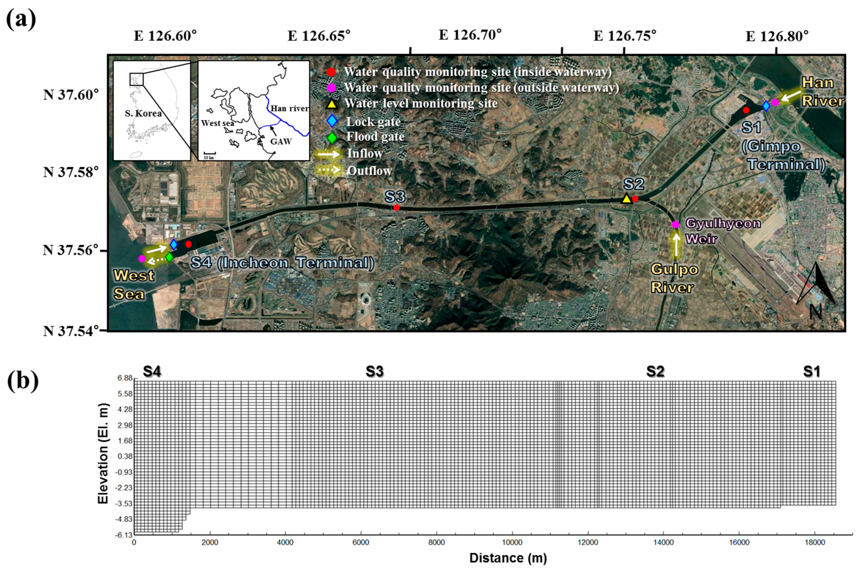
GAW is South Korea’s first navigational waterway artificially constructed to connect the West Sea and Han River. It is located in the northern part of South Korea between the cities of Incheon and Seoul (the South Korean capital). GAW was originally designed to prevent chronic flooding around the Gulpo River region, but was redesigned to serve as both a transport route and a flood prevention facility. The main components of the waterway include an 18-km-long navigation channel (width: 80 m, operating depth: 6.3 m) connecting terminals (T/Ms) at Incheon (area: 2.84 km2) and Gimpo (area: 1.91 km2), and lock gates at each end (Figure 1a). Additional structures include a diversion culvert and weir where the Gulpo River joins GAW. GAW transports seawater from the West Sea and freshwater from the Han River (through lock gates at the ends of the two terminals), and discharges water through the flood gate of the Incheon T/M. The Gulpo River is normally diverted to the Han River, and flows into the waterway only when the Gyulhyeon Weir is overflowing because of rainfall. The quantity of the saltwater from the West Sea is approximately twice that of the freshwater from the Han River. Therefore, a brackish water zone is artificially formed in the waterway. The tidal cycle range in the West Sea area, which is adjacent to the Incheon T/M, is between sea level +5.30 and −4.45 EL. m, and the waterway operation level is EL. 2.7 m. Accordingly, there are periods during the tidal cycle when water flows both into and out of the waterway. As a result of these large water level fluctuations and changes in flow direction, the waterway exhibits spatially complex hydraulic characteristics.
Although the basin area of GAW (including the Gulpo River area) does not exceed 134 km2, the Han River flowing in from the Gimpo T/M has a very large basin area of 25,953 km2. Further, as the Han River flows through Seoul, the country’s capital with a population exceeding 10 million, its pollution levels are usually high. The Gulpo River flows into the waterway in the case of flooding only. However, the majority of the inflow is from urban WWTPs. Therefore, the Gulpo River has the poorest water quality among the three inflow sources (the Han River, West Sea, and Gulpo River). Consequently, GAW is eutrophic year-round, which causes water quality problems such as algal bloom and DO depletion. Furthermore, as fish enter the waterway when the rock gates are opened, the waterway has a very peculiar environment in which freshwater, brackish, and saltwater fish species are observed simultaneously.
2.2. Survey of Water Quality and Fish
2.2.1. Water Quality
The GAW water quality was surveyed on a weekly basis from January to December 2014. The inflow water outside the waterway was monitored once a week at three sites, namely the Han River (outside the Gimpo T/M lock gate), Gulpo River (the upper region of Gyulhyeon Weir), and the West Sea (outside the Incheon T/M lock gate). Similarly to the case of the outside waterway, the water quality of the navigational channel was monitored weekly at four main sites, namely Gimpo T/M (S1), Gyeyang Bridge (S2), Sicheon Bridge (S3), and Incheon T/M (S4) (Figure 1a). Inflow water samples were collected from the surface layer using a Van Dorn water sampler. In the channel, samples were collected at 1, 3, and 5 m depth, corresponding to the surface, middle, and bottom layers, respectively. A water quality measurement instrument (YSI EXO1, Yellow Spring Instrument Inc.) was used to measure the water temperature, DO, salinity, pH, conductivity, and turbidity during the sampling. The chlorophyll-a (Chl-a), phosphate (PO4-P), nitrate (NO3-N), ammomium (NH4-N), total phosphorus (TP), and total nitrogen (TN) levels were analyzed using the standard method [25].
2.2.2. Fish
The fish abundance data for GAW used in this study were based on an environmental impact assessment survey by K-water [26]. The investigation was conducted in each season of 2014 at the four water quality monitoring sites of the waterway and in the Han and Gulpo Rivers. Details of sampling methods are provided in Appendix A.
2.3. Model Selection and Description
The CE-QUAL-W2 model is a two-dimensional laterally averaged hydrodynamic and water quality model co-developed by the U.S. Army Corps of Engineers Waterways Experiment Station and Portland State University [27]. Because the model assumes lateral homogeneity, it is best suited for relatively long and narrow waterbodies exhibiting longitudinal and vertical water quality gradients. This model has been applied to various stratified lakes and reservoirs worldwide [28,29,30,31,32]. In particular, Park et al. [33] and Brown et al. [34] have shown successful application of this model to estuaries. The CE-QUAL-W2 version 4.0 model was selected in this study because it is appropriate for GAW, for which the lateral variations in water quality are unimportant but the vertical variations in velocity, salinity, and DO are significant. CE-QUAL-W2 is based on finite difference solution of the laterally averaged equations of fluid motion, including the continuity equation, x-momentum equation, z-momentum equation, free surface equation, equation of state, and advective–diffusion equation. Details of these equations are provided in Appendix B.
2.4. Configuration and Application of Model
The geographical model of GAW constructed by CE-QUAL-W2 is illustrated in Figure 1b. The model grid consisted of 173 segments and 52 layers in the water depth direction. The average segment length was 103 m and the layers were finely distinguished at a vertical spacing of 0.25 m. For the inflow/outflow data, the GAW water management system (ARAWMS) constructed and input datasets representing inflow from the West Sea, Han River, and Gulpo River and datasets representing outflow through the West Sea flood gate at hourly intervals. The water quality of the inflow from the three sources was monitored every week, and the survey results were input to establish the water quality boundary conditions. The 12 constituents taken as the boundary conditions of CE-QUAL-W2 were the chemical oxygen demand (CODMn), salinity, suspended solid (SS), PO4-P, NH4-N, NO3-N, labile dissolved organic matter (LDOM), refractory dissolved organic matter (RDOM), labile particulate organic matter (LPOM), refractory particulate organic matter (RPOM), algae, and DO. Observational data recorded at the Incheon meteorological station of the Korean Meteorological Administration were used to calculate water temperatures [35]. The hourly temperature, wind direction, velocity, dew-point temperature, and cloudiness data were configured as input files. The simulation was conducted from January to December 2014 so that seasonal variation could be reflected. The minimum and maximum computational time steps were set to 1 and 3600 s, respectively. Within the assigned value, the average time step equaled 61 s in the range of 2–98 s. Table 1 presents the hydraulic and water quality parameters used for calibrating the CE-QUAL-W2 model.
2.5. Model Performance Assessment
The model performance was assessed using the root mean square error (RMSE) and absolute mean error (AME). These statistics are frequently used to examine the goodness of fit between modeling results and observed values. They were calculated using the following equations:
where n is the number of measured and predicted pairs, O is an observed value, and P is a predicted value.
3. Results and Discussion
3.1. Field Survey
3.1.1. Comparison of Inflow Rate and Water Quality
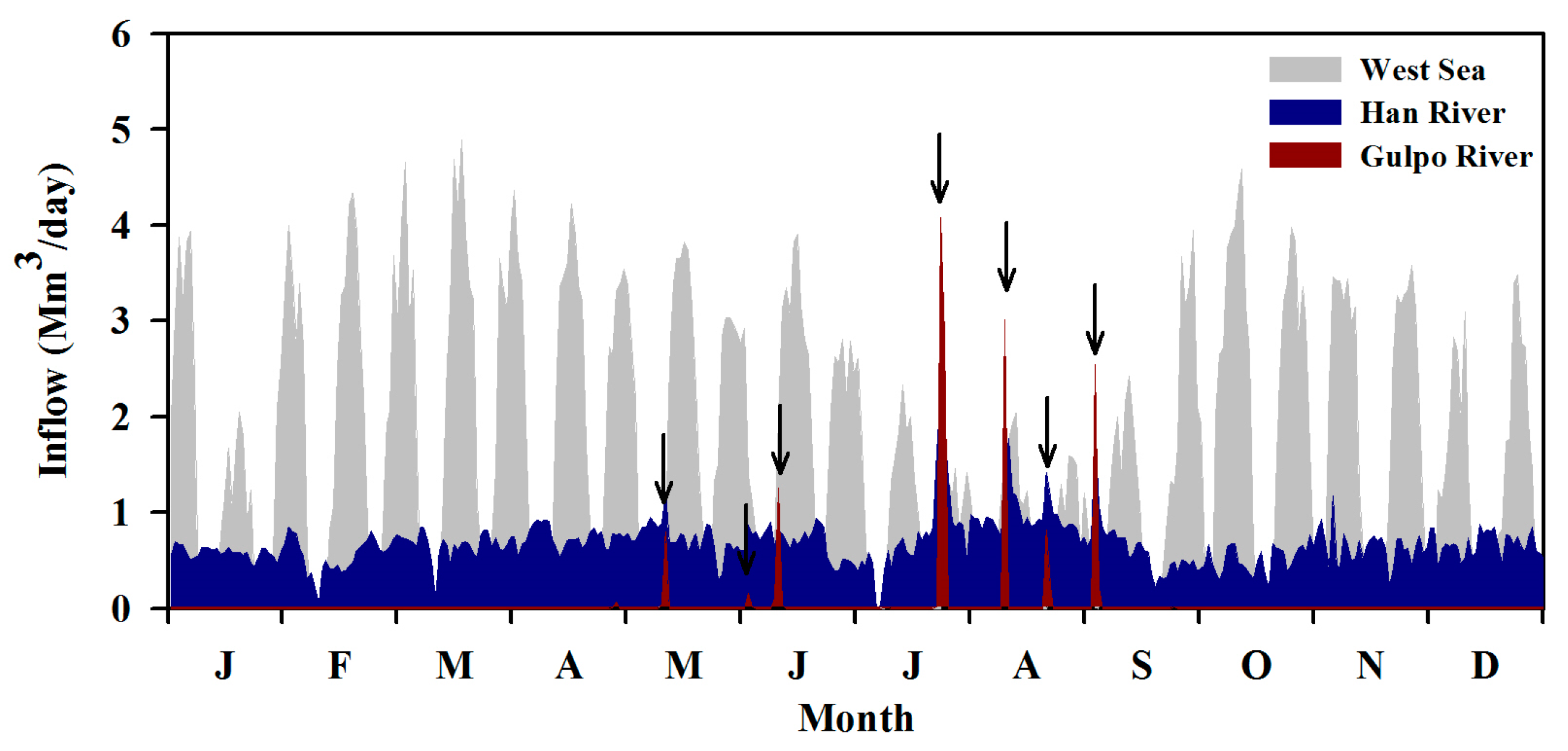
Figure 2 shows the total inflow of GAW in 2014. The West Sea provided the largest annual inflow of 597.8 × 10⁶ m3, followed by 247.2 and 16.3 × 10⁶ m3 from the Han River and Gulpo River, respectively. As for the relative proportions of annual inflow, the Han River, Gulpo River and West Sea accounted for 28.7%, 1.9%, and 69.4%, respectively. The Gulpo River is only diverted to the GAW navigational channel when Gyulhyeon Weir overflows because of heavy rainfall; this occurred seven times during the study period. The inflow from the West Sea showed a remarkable tidal fluctuation during the spring and neap tides. During the neap tides, inflow did not occur for 2 to 5 consecutive days twice a month. In addition, the inflow decreased from July to August due to flood control. In contrast, the Han River exhibited a relatively constant inflow rate throughout the year.
Table 2 presents the water quality parameters of the inflow water during the study period. As regards the annual average concentration of organic matter, the Gulpo River had a CODMn of 12.4 mg/L, which far exceeded the 5.8 and 2.8 mg/L values for the Han River and West Sea. As regards the nutrient concentrations, the Gulpo River exhibited a TN of 12.196 mg/L and TP of 2.553 mg/L, indicating a strongly eutrophic state. The standard deviations were also large. Accordingly, because of the influence of these high concentrations of organic matter and nutrients, the DO in the Gulpo River was as low as 5.2 mg/L. The highest salinity level of 25.7 psu was recorded in the West Sea, while low salinity was observed for other rivers. The highest Chl-a level of 21.7 μg/L was recorded in the Han River. The Gulpo River, which had the poorest water quality, featured a lower level of Chl-a than the Han River because of dilution with water discharged from WWTPs. With the exception of the flood season, WWTP discharge accounted for almost 70% of the Gulpo River flow.
3.1.2. Salinity Stratification and DO Depletion
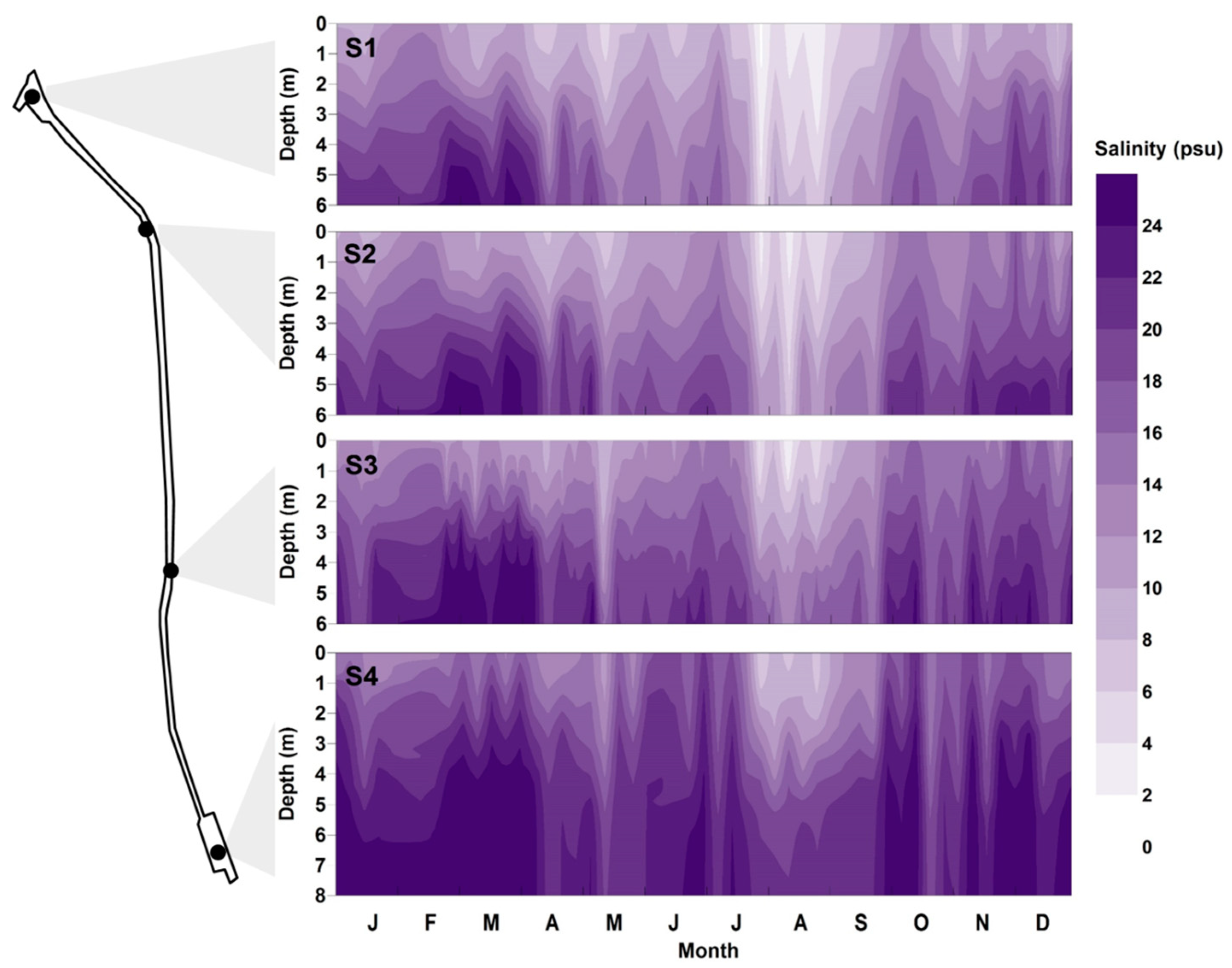
The salinity and DO were monitored in the vertical direction at each monitoring site. Various spatial distributions appeared to depend on the inflow and distance from each source. When there was considerable inflow from the West Sea, the salinity was high in the bottom layer and the strong salinity stratification was created (Figure 3). The highest salinity was measured at S4, which was adjacent to the West Sea, while the lowest salinity was recorded at S1, which was at the entrance of the Han River. When inflow from the Gulpo River occurred, the salinity decreased dramatically. This phenomenon was observed in May, July, and August. The lowest salinity values of the year were obtained from July to early September, because of the inflow from the Gulpo River and the decrease in the inflow from the West Sea. From the middle of September, the inflow from the West Sea increased, such that the previous salinity and stratification levels were reestablished.
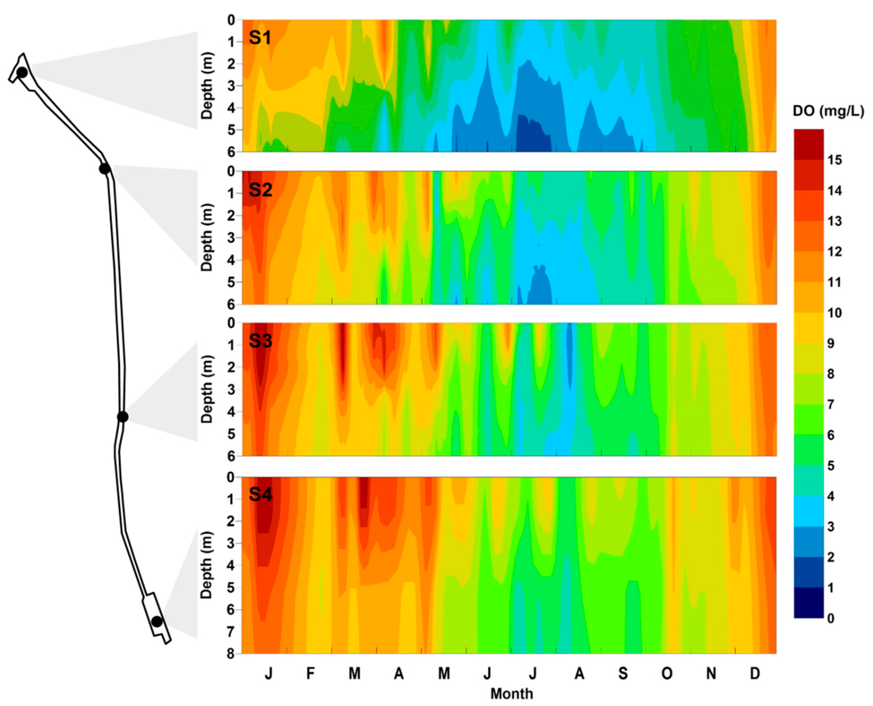
The spatial and seasonal variations of the DO concentration were more drastic than those of the salinity (Figure 4). DO was more abundant during seasons with lower water temperature (from January to April and from October to December). On the other hand, the DO concentration decreased dramatically from May to September. In May, the DO concentration began to decrease in the bottom layer rather than the surface layer. During summer, the vertical gradient of the DO concentration among the water layers was clear; it began to decrease in October. The most serious DO depletion was recorded at S1. However, greater proximity to the West Sea corresponded to higher DO concentration. At S1, a DO of 3 mg/L or lower persisted for approximately five consecutive months (from May to September) and hypoxia (<2 mg/L), occurred during the month of July. Hypoxia was also observed at S2, which was closest to S1. Lower frequencies of DO depletion were observed at S3 and S4. However, from July to August and in September, during which the inflow from the West Sea decreased, the DO concentration decreased dramatically because of the impact of the S1 hypoxia. In other words, the hypoxia occurring in the upper regions from Gimpo T/M spread towards the Incheon T/M area when the current from the West Sea was less influential. The formation time of the hypoxic zone of GAW was similar to other esturine systems (e.g., Chesapeake Bay, Gulf of Mexico, and Tokyo Bay) owing to the increase in temperature and reduction of oxygen saturation in the summer [14,15,16,17,36,37,38]. In particular, there was a similarity in the spatial distribution of the hypoxic zone in the St. Lucie Estuary (USA) and Gironde Estuary (France), which are both affected by river discharge and have narrow width and low water depth. These estuaries were affected by a high concentration of nutrients entering the river, and thus, severe oxygen depletion occurred near the water zone adjacent to the river [11,13].
3.2. Model Validation
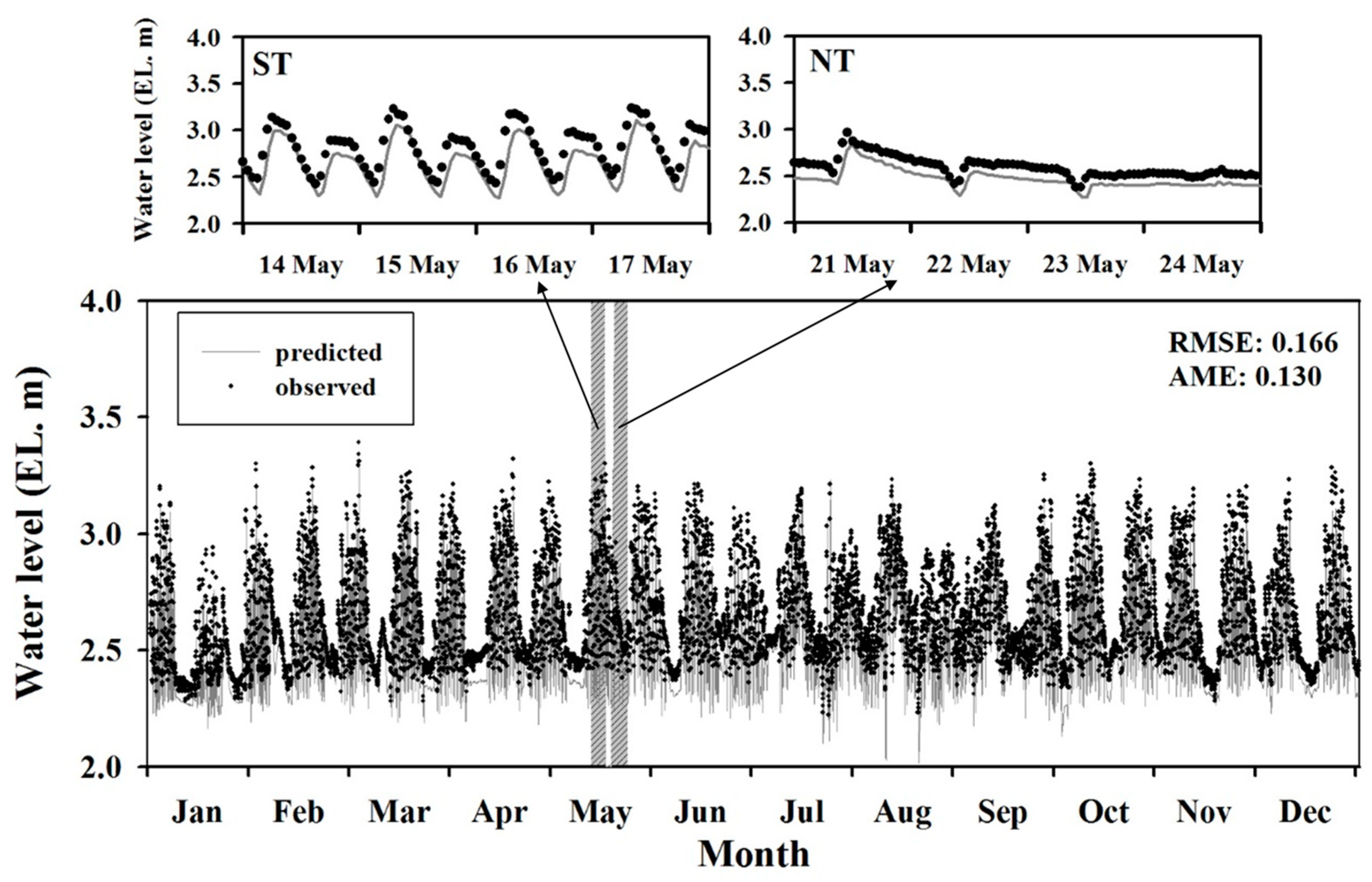
The spatiotemporal variations of the salinity stratification, DO depletion, and other water quality parameters were simulated using CE-QUAL-W2. The observed water levels were compared with predicted values to determine whether the model could accurately represent the water level variation in the navigational channel under the tidal influence (Figure 5). Although the predicted water levels were in relatively good agreement with those observed in practice, the model tended to overestimate the water level of GAW, particularly in the cases of low and neap tides, and RMSE/AME were determined as 0.166/0.130 m, respectively. Since the boundary conditions of the model were implemented at the external/internal flow rather than at the water level, the error of the observed flow affected water level calculations.
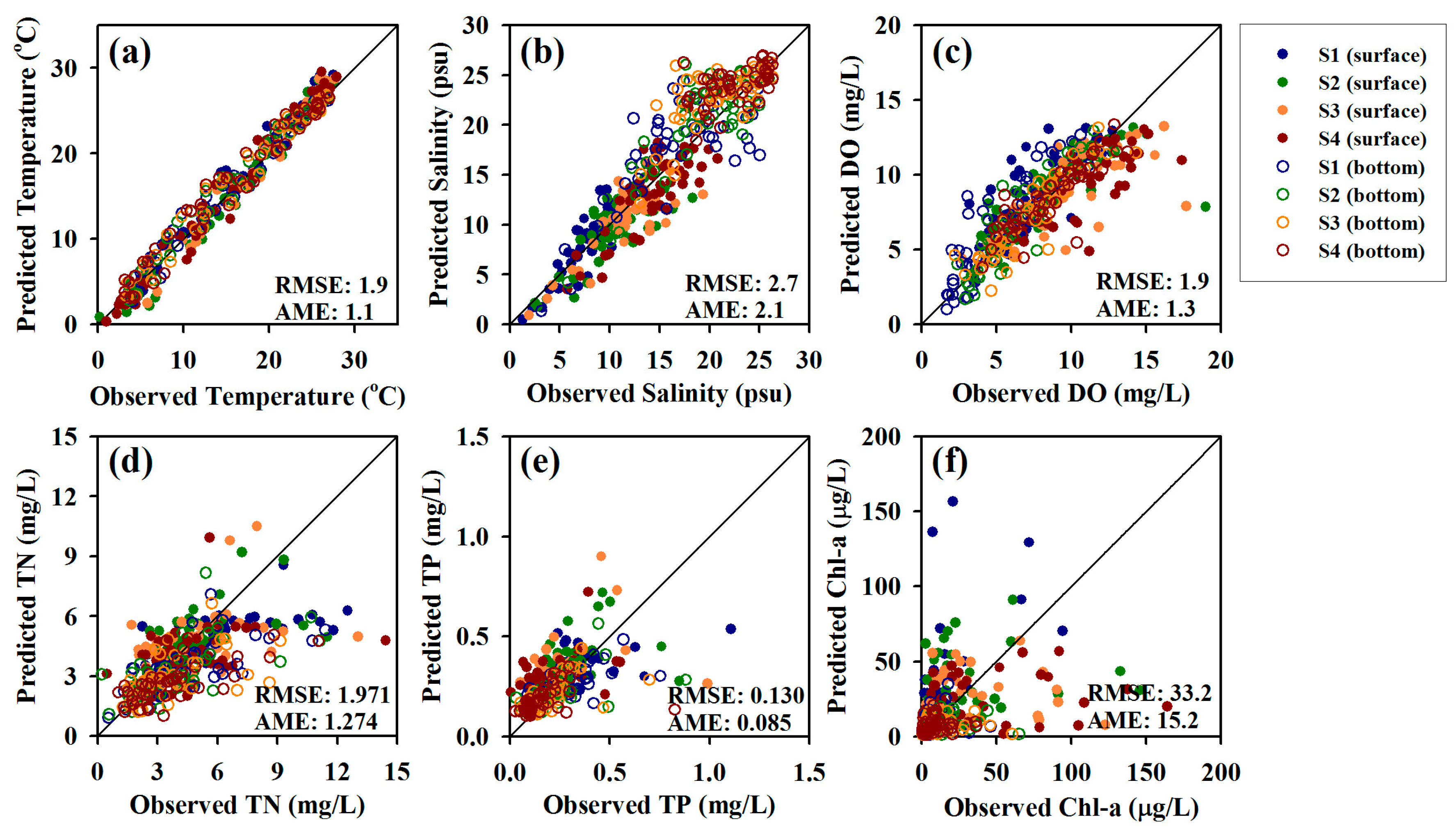
Figure 6 illustrates the validation results for water quality constituents in the surface and bottom layers. The RMSEs of temperature, salinity, and DO were relatively low (1.9 °C, 2.7 psu, and 1.9 mg/L, respectively), i.e., the developed model realistically reproduced the water quality levels of the waterway. As for nutrient concentration, the RMSE and AME of TN levels were determined as 1.971 and 1.274 mg/L, respectively, while the corresponding values for TP were obtained as 0.130 and 0.085 mg/L, respectively. High concentrations were mainly underestimated by the model, but the overall variation was reproduced relatively well. Chl-a simulation results yielded an RMSE of 33.2 μg/L and an AME of 15.2 μg/L. Overestimation occurred at S1 and S2, while underestimation was detected at S3 and S4, which indicated an increase of the error range. The low accuracy of Chl-a level prediction was ascribed to model limitations. In particular, the model cannot distinguish between marine and freshwater algae species during Chl-a simulation. In GAW, freshwater and marine algae are affected by high and low salinity, respectively, but the used model does not consider salinity as a limiting factor for algal growth. These limitations affected the accuracy of the Chl-a prediction as well as the prediction accuracy of the DO concentration in the surface layer. Figures S1 and S2, as supplementary documents, provide time-series comparisons of observed and predicted values at the surface and in the bottom layer.
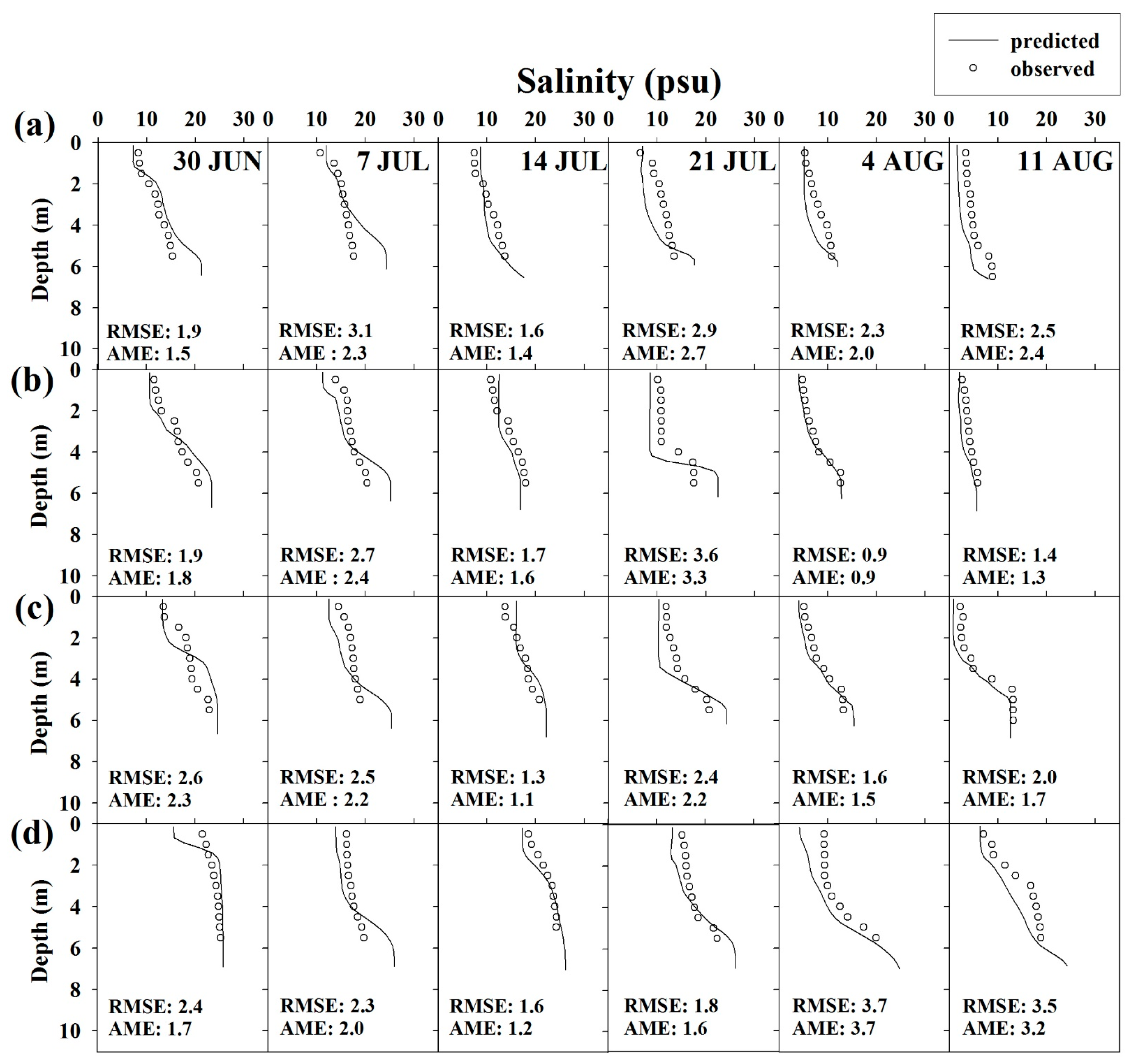
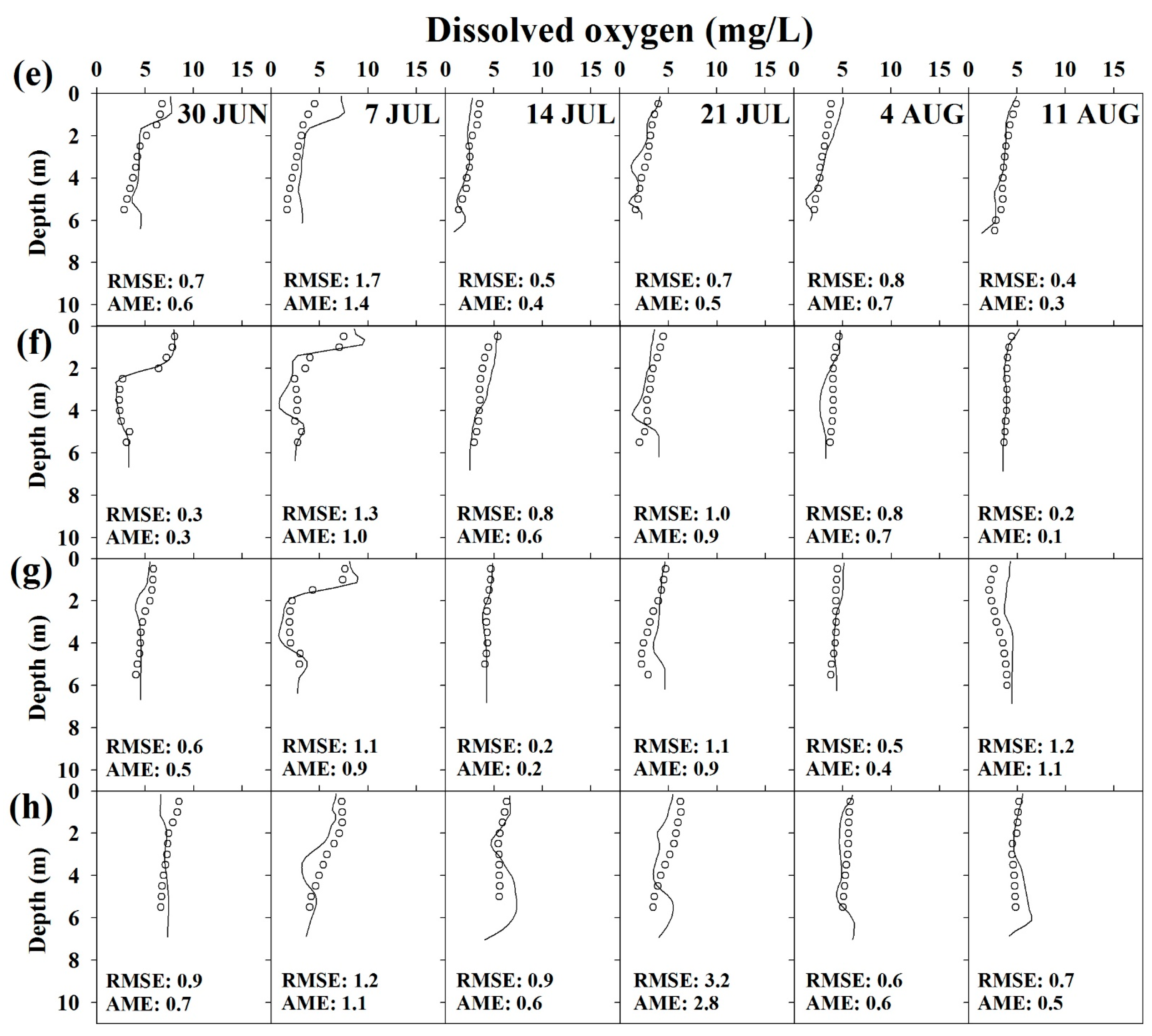
The simulation results for the vertical salinity and DO concentration are discussed with a focus on summer, when the DO depletion was serious (Figure 7). Validation results reveal that the vertical distributions of salinity and DO concentration were relatively well reproduced by the model. In particular, an RMSE of 0.9–3.7 psu and an AME of 0.9–3.7 psu were obtained for salinity modeling, i.e., the corresponding error range was small. The model also suitably simulated salinity stratification caused by density differences and the spatial distribution of concentration (differences in concentrations at S1, S2, S3, and S4 on the same day). For DO modeling, error ranges were determined as 0.2–3.2 mg/L (RMSE) and 0.1–2.8 mg/L (AME). Thus, the model was appropriately validated. In particular, summer hypoxia at S1 (Figure 7e) and DO depletion due to the spread of hypoxia to S4 (Figure 7h) were relatively well reproduced.
3.3. Physical Factors Affecting Hypoxia Formation
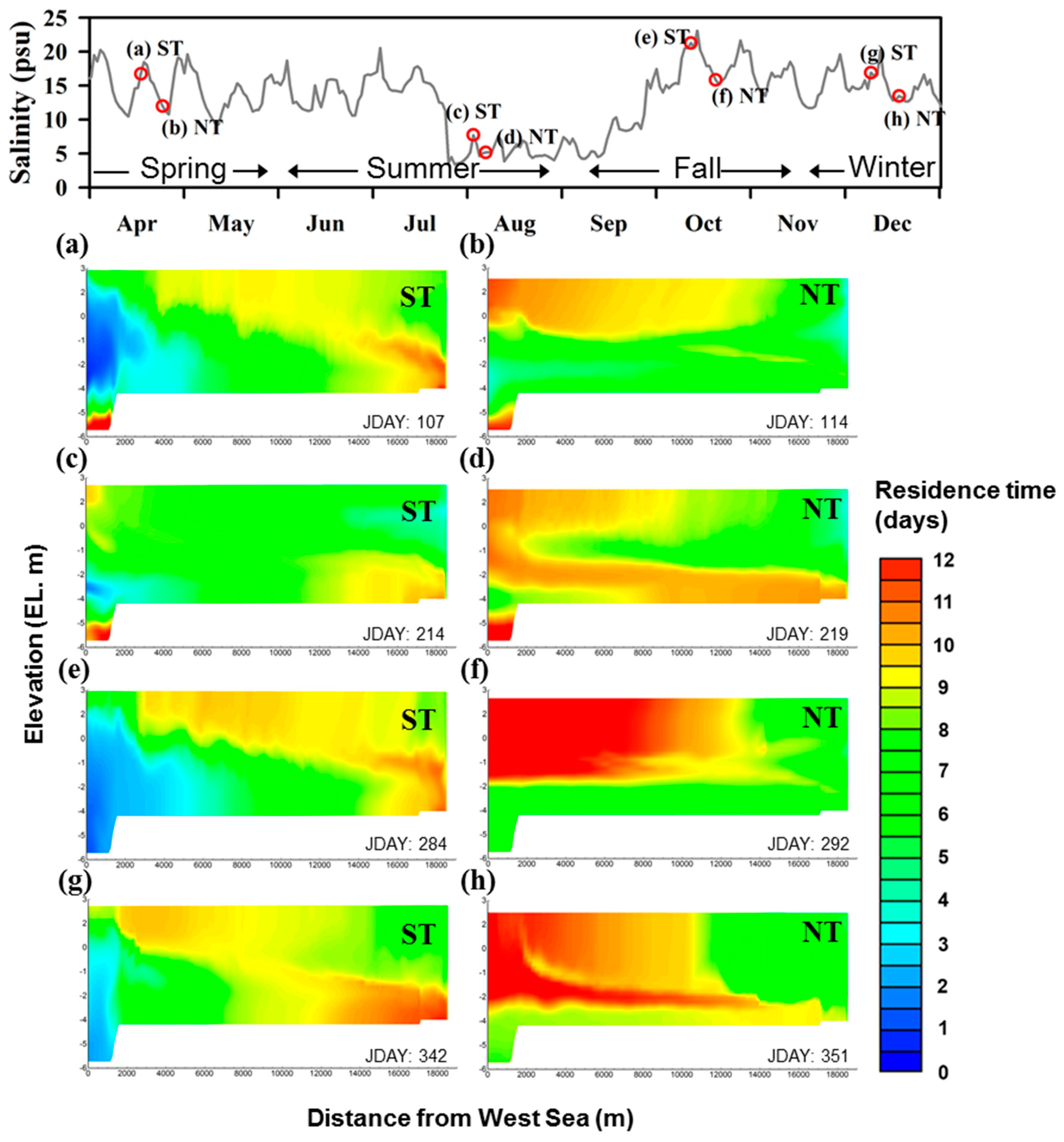
To analyze the physical factors affecting the hypoxia formation, the residence time and salinity distributions during the spring and neap tides were examined. In this study, the residence time was defined as the period during which water coming from the boundary remains in the waterbody and was calculated by setting the zero-order decay rate to −1 day−1 and zeroing out all other generic constituent kinetic parameters [27]. In each season, the time difference between a spring tide and a neap tide was between 5 and 9 days. However, there was a stark difference in the spatial distribution of the residence time (Figure 8). During the spring tide, when the inflow from the West Sea peaked, the residence time was shortest at S4 and longest at S1 (Figure 8a,c,e,g). In particular, the bottom layer of S1 exhibited the most stagnant characteristics. This waterbody with the longest residence time was mixed with the inflow from the Han River and spread to the upper layers of S2 and S3. On the other hand, during the neap tide, the West Sea provided no saltwater and the current from the Han River became stronger. Accordingly, the stagnant water mass in the bottom layer of S1 spread to the upper layer of S4 through S2 and S3 (Figure 8b,d,f,h). However, during summer, the bottom layer of S1 continuously exhibited a long residence time. This behavior seems to have occurred because the velocity of the stagnant water mass decreased as the discharge was reduced in accordance with the decreased inflow from the West Sea. Analysis revealed that this residence time spatial distribution created a physical environment in which the strongest hypoxia occurred at S1. Therefore, this simulation result indicates that the physical environment of the waterway undergoes a very drastic change in both time and space, and this feature greatly affects the water quality and ecosystem.
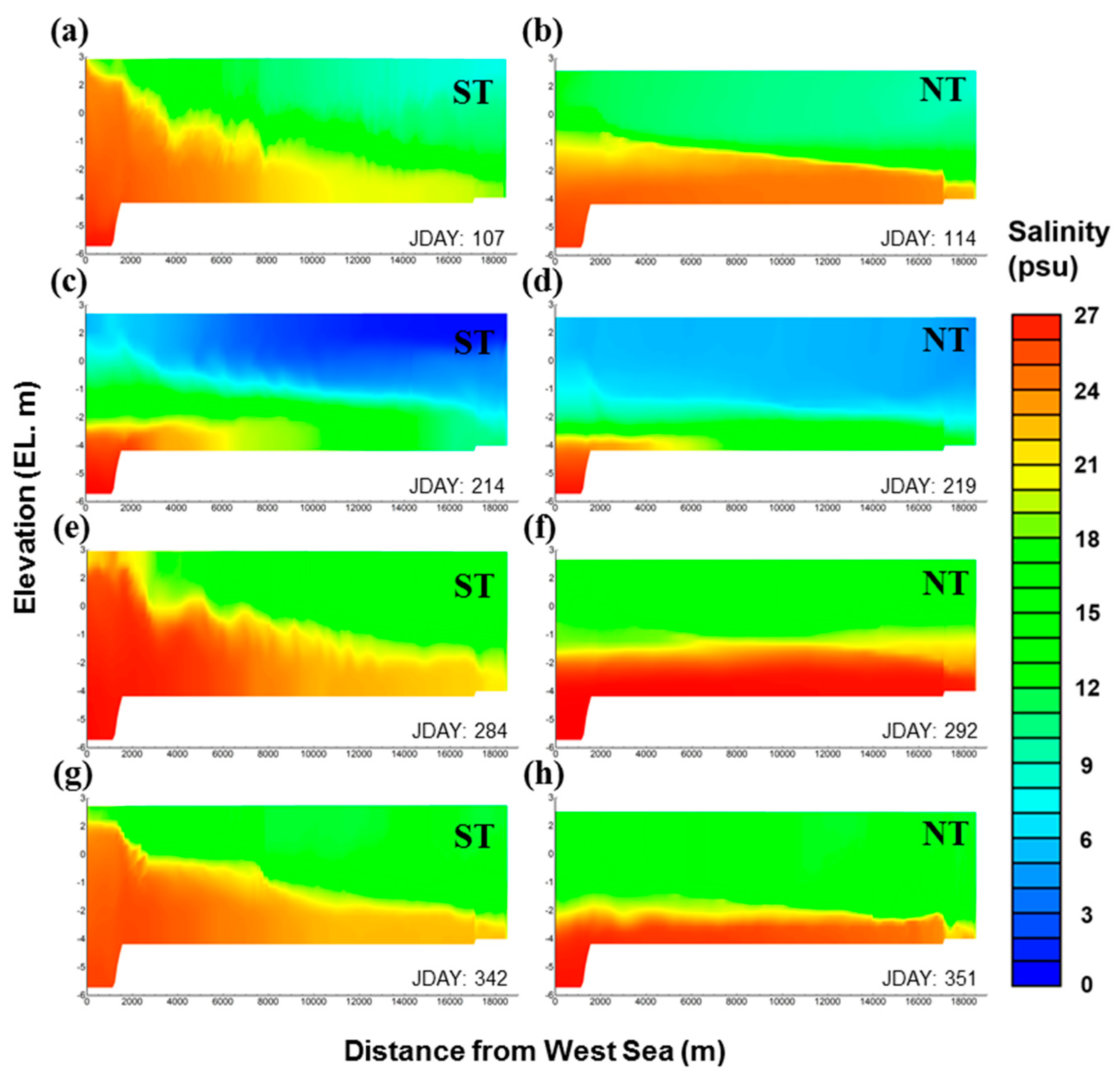
The variation in the salinity distribution was more strongly affected by the change of inflow during the spring and neap tides than by seasonal change (Figure 9). During the spring tide, the inflow from the West Sea increased and, thus, the salinity increased dramatically. For this reason, a saltwater wedge typical for an estuary occurred in the navigational channel. During the neap tide, saltwater tended to concentrate in the bottom layer, exhibiting slow movement. In general, the spring and neap tides in spring, autumn, and winter yielded similar salinity spatial distributions. On the other hand, during summer, as the inflow from the West Sea decreased, the salinity of the upper layer decreased to 10 psu or below, thereby causing freshwater dominance.
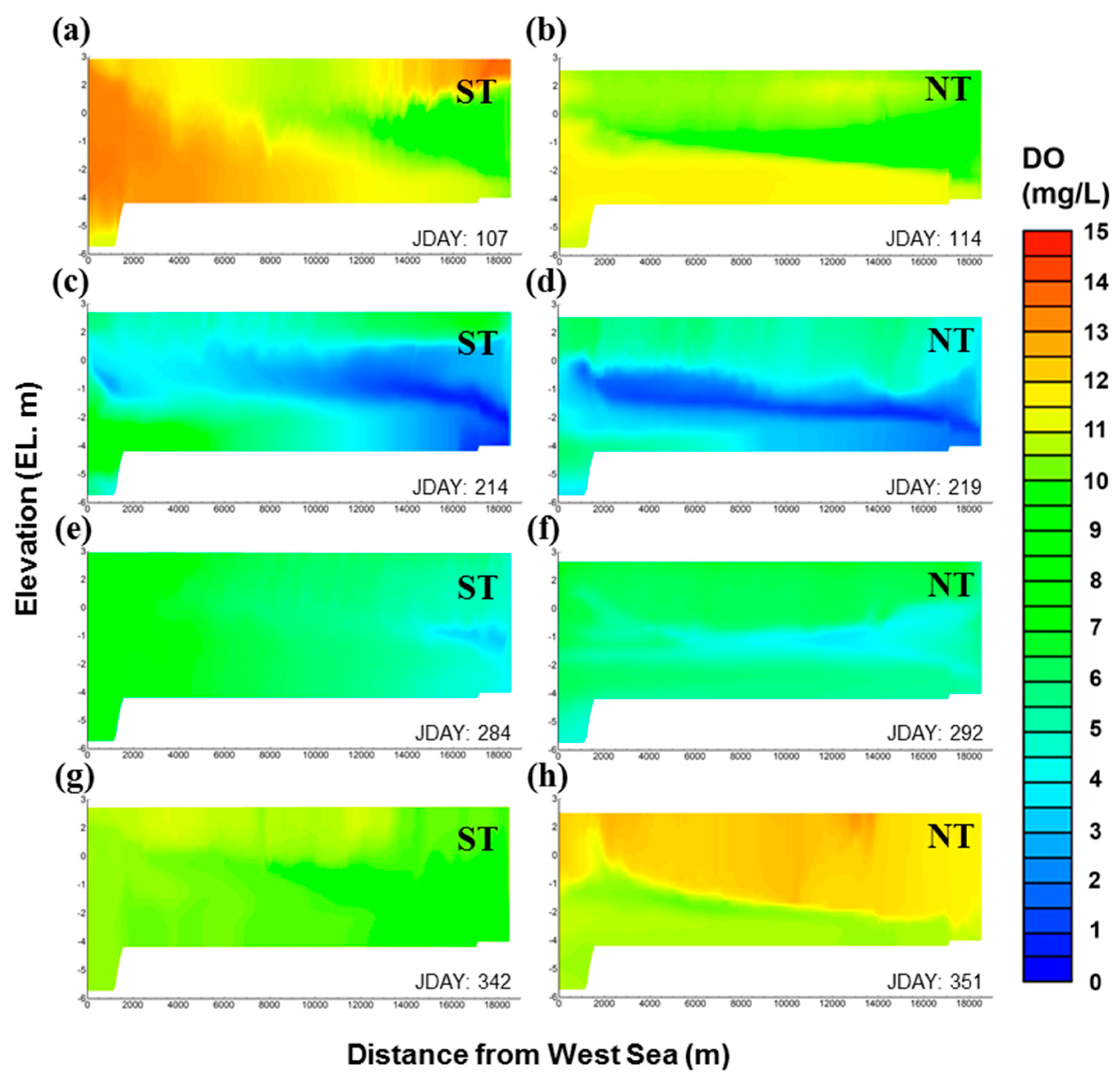
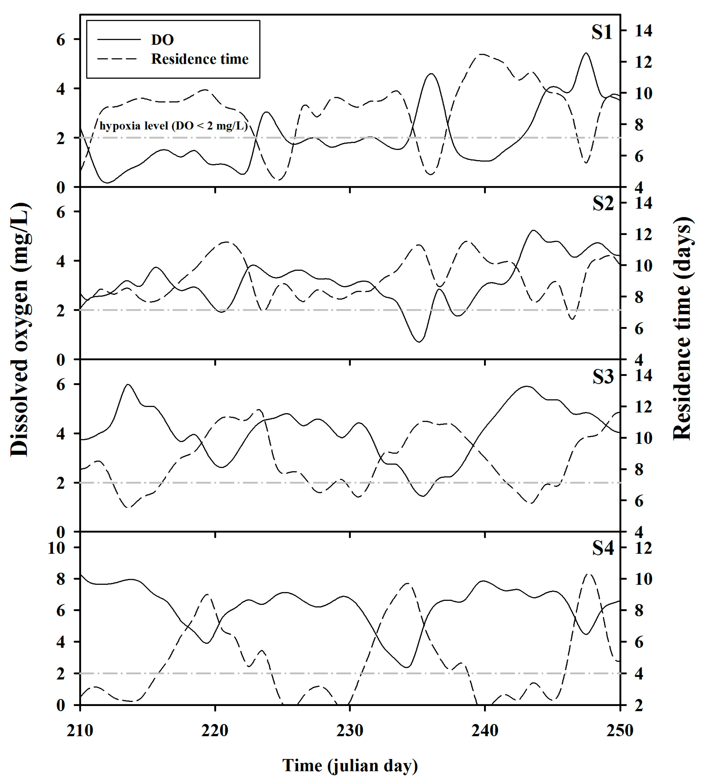
Figure 10 presents the simulation result for the DO spatial distribution. It seems that the DO concentration distribution was affected by not only the above-mentioned physical factors such as residence time and salinity stratification, but also other complex factors such as water temperature and organic matter decomposition. The model accurately simulated the frequent DO depletion in the bottom layer of S1 and also revealed the spread of the hypoxia generated at S1 towards S4 during the neap tide. In particular, as shown in Figure 10c,d, the hypoxic waterbody in the bottom layer migrated to the middle layer, and the so-called metalimnetic oxygen minima were predicted. This behavior was ascribed to the fact that the operation of the Gimpo terminal only allows freshwater inflow into the Han River while blocking discharge into the Han River, which results in the migration of the hypoxic waterbody mixed with fresh water to the middle layer. As a result, stagnant zones are generated in the waterbody, which yield hypoxic zones exhibiting DO depletion. This behavior is well illustrated by the time-series comparison of residence time and DO values at the bottom of each site (Figure 11). Temporal changes in DO concentration and residence time clearly showed opposite trends in the bottom layer. Notably, these trends were significant at S1, S3, and S4 but relatively insignificant at S2, which was ascribed to the fact that at S2, the influence of the inflow of the Han River and the West Sea was offset by two-way flow. Consequently, the simulation results showed that GAW has the anthropogenic characteristics of estuarine water and, thus, a unique aquatic environment in which the physical conditions and water quality change dramatically during spring and neap tides. The inflow is artificially controlled, but is also affected by tides. In addition, there are two or three inflow sources, but discharge occurs in one direction only.
Studies on hypoxia formation in the Chesapeake Bay, the Gulf of Mexico, and the Tokyo Bay have examined the influence of wind on hypoxia in various ways [14,15,16,17,36,37,38,39,40]. The intensity and direction of the wind were evaluated as the main factors influencing the formation and duration of the hypoxic layer. In this study, however, the effect of wind on the stratification and depletion of DO in GAW could not be evaluated, and further study is needed. Further, many studies on the hypoxia formation in Lake Erie have quantitatively evaluated the effect of nutrient loading. Scavia et al. [39] and Rucinski et al. [40] suggested that the reduction of phosphorus may reduce the hypoxia area of the Lake Erie. Considering these prior studies, the reduction of nutrients from the Han River and the Gulpo River may have the potential to reduce hypoxia in GAW, and therefore, additional research is needed.
3.4. Assessment of Fish Habitat Volume
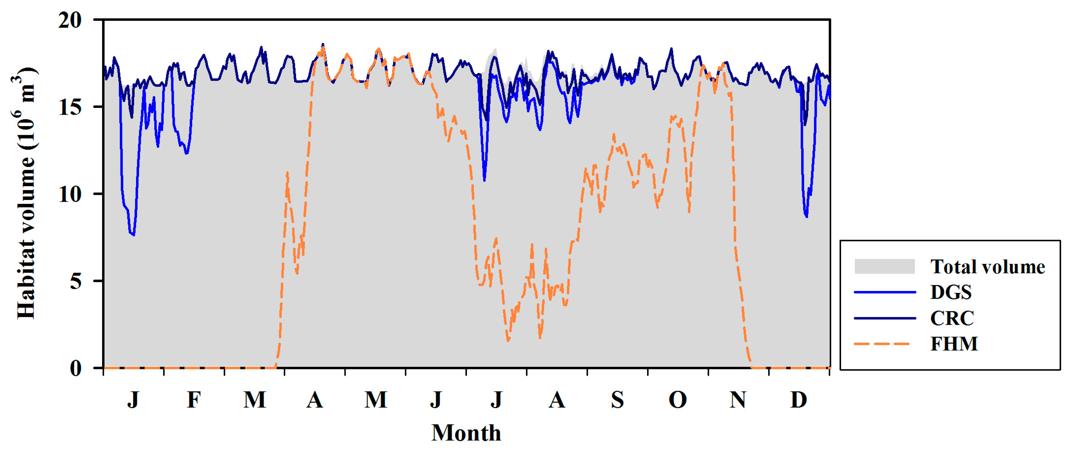
The fish numbers surveyed in each season of the study period are presented in Appendix A [26]. In this study, three main fish species were selected, and their habitat environments were investigated in order to determine habitat volumes in relation to temperature and DO (Table 3). As the habitat volumes, the minimum habitat conditions for survival were considered instead of the optimal conditions. Except for the crucian carp (CRC), the other three species were selected because they were frequently observed at every site (S1–S4). In contrast, CRC appeared at S1 only. However, many CRCs live in the Han and Gulpo Rivers and are likely to enter the waterway with freshwater flows. Therefore, CRC was included in the main fish species, since its habitat encompasses regions with broadly variable temperature. Their habitats also have very low DO limit concentrations. Accordingly, these species can endure hypoxia well. The dotted gizzard shad (DGS) also has a wide habitat range, while the flathead mullet (FHM) was observed to have a narrow habitat range and has a low tolerance for DO depletion.
Figure 12 presents the fish habitat volumes for each fish species calculated using the model, revealing that CRC could survive in every volume irrespective of season. However, the DGS habitat volume decreased between January and February and in December, when the water temperature decreased dramatically, and between July and August, when strong hypoxia occurred. FHM was most sensitive to environmental change. This species had few habitat volumes for survival between January and March and in December, when the water temperature was low. In late June, its habitat volume was reduced to 77% of the total water volume as a result of hypoxia. Furthermore, the average habitat volumes for survival were restricted to 34% and 32% in July and between August and September, respectively.
Analysis of the fish habitat volumes yielded by the simulation revealed the following: if a fish species sensitive to hypoxia enters the waterway, a poor habitat environment could be maintained for a long period of time. Recall also that the habitat volumes calculated in this study correspond to the minimum habitats for survival, and the optimal habitat volumes are considerably more limited. Besides, as the calculations did not distinguish between life stages, the survival behavior for the larvae and juvenile stages would be more limited.
The modeling results of this study revealed that GAW with its artificial estuarine environment produces hypoxia due to continuous eutrophic inflow and slow physical circulation. Moreover, as the waterway exhibits very complex waterbody behaviors, simulation-based prediction of spatiotemporal production and the spread of hypoxia seems essential. In order to maintain a sound aquatic environment, fish habitats must be assessed continuously. It is expected that the model employed in this study will be effectively utilized to derive operational measures for GAW, which could increase habitat volumes.
4. Conclusions
This study analyzed the effect of hydraulic and water quality factors on the spatiotemporal formation of summer hypoxia in GAW, an artificial estuarine waterway, by applying the two-dimensional CE-QAUL-W2 hydrodynamic and water quality model. In addition, the ecological vulnerability of major fish species to hypoxia was determined, by calculating habitat volumes in relation to temperature and DO.
The salinity and DO of GAW were monitored throughout the year 2014, in both the horizontal and vertical directions. Various spatial distributions were obtained according to inflow and distance from each inflow source. The salinity level was highest at the Gimpo connecting terminal (S4) and lowest at the Incheon connecting terminal (S1). When the inflow from the West Sea increased, the salinity stratification increased. DO was more abundant when the water temperature was low. However, during summer, the concentration gradient among the water layers became clearer and hypoxia was observed. The longest period of hypoxia was observed at S1. When the inflow from the West Sea decreased, the hypoxia at S1 seemed to be spread towards S4.
The simulation results showed that the CE-QAUL-W2 model realistically reproduced the water quality characteristics of GAW. Both the salinity and DO were relatively well simulated with error rates of RMSE 2.7 psu and 1.9 mg/L, respectively. The simulation results for the vertical salinity and DO also indicated that the salinity stratification, vertical DO gradient, and summer hypoxia were very accurately reproduced.
To analyze the physical factors affecting the hypoxia generation, the residence time, salinity, and DO concentration distributions during the spring and neap tides were comprehensively analyzed for each season. The bottom layer of S1 exhibited the longest residence time, which seemed to be the greatest physical factor influencing hypoxia. This waterbody with limited circulation spread towards S4 during summer and the neap tide, when the inflow from the West Sea decreased. These simulation results provided a basis for identifying the drivers of the observed DO depletion and enabled satisfactory explanation of the generation and distribution of hypoxic zones. The simulation results also clarified that GAW has a unique aquatic environment, with physical conditions and water quality levels that change dramatically according to the tidal flow (inflow and outflow) regulation.
Finally, the fish habitat volumes for survival were calculated. The flathead mullet was found to be most sensitive to environmental change. In summer, the habitat volume of this species was limited to 32–34% of the total volume as a result of hypoxia. Note that, if life stages were considered, the survival habitat volume of this species would be further reduced; therefore, hypoxia countermeasures are required. In order to maintain a sound aquatic environment, fish habitats must be continuously assessed in further studies. The model employed in this study can be effectively utilized to derive operational measures for GAW, with the potential to increase habitat volumes.
Supplementary Materials
The following are available online at https://www.mdpi.com/2073-4441/10/11/1695/s1, Figure S1: Comparisons of predicted and observed water quality constituents in the surface layer, Figure S2: Comparisons of predicted and observed water quality constituents in the bottom layer.
Author Contributions
Conceptualization, S.C. and K.-G.A.; Methodology, S.C. and C.P.; Software, S.C.; Validation, S.C.; Formal Analysis, S.C. and K.R.L.; Investigation, K.R.L. and C.P.; Resources, K.R.L. and C.P.; Data Curation, K.R.L.; Writing-Original Draft Preparation, S.C.; Writing-Review & Editing, K.-G.A.; Visualization, S.C.; Supervision, K.-G.A.; Project Administration, S.C.
Funding
This research was supported by K-water.
Acknowledgments
The authors would like to thank the reviewers for their detailed comments and suggestions for the manuscript.
Conflicts of Interest
The authors declare no conflict of interest.
Appendix A

Table A1.
Results of freshwater, brackish, and saltwater fish survey in 2014. Fish were caught using both catching nets (mesh size: 5 mm × 5 mm) and kick nets (mesh size: 4 mm × 4 mm), and the catch per unit effort (CPUE) method was adopted for quantitative collection. Gill nets (mesh size: 25 mm × 25 mm, length: 25 m) were also installed for the investigation. (M: March, J: June, S: September, N: logNovember).
| Monitoring Sites | S1 | S2 | S3 | |||||||||
| Family/Species | M | J | S | N | M | J | S | N | M | J | S | N |
| Family Anguillidae | ||||||||||||
| Anguilla japonica | ||||||||||||
| Family Engraulidae | ||||||||||||
| Coilia nasus | 2 | |||||||||||
| Engraulis japonicus | 4 | |||||||||||
| Thryssa kammalensis | 31 | 15 | 19 | 22 | ||||||||
| Family Clupeidae | ||||||||||||
| Konosirus punctatus | 46 | 37 | 16 | 9 | 117 | 43 | 17 | 168 | 74 | |||
| Family Cyprinidae | ||||||||||||
| Acanthorhodeus macropterus | ||||||||||||
| Acheilognathus lanceolata intermedia | ||||||||||||
| Carassius auratus | 2 | 1 | ||||||||||
| Cyprinus carpio | ||||||||||||
| Erythroculter erythropterus | ||||||||||||
| Hemibarbus labeo | 1 | |||||||||||
| Hemiculter leucisculus | ||||||||||||
| Saurogobio dabryi | 1 | |||||||||||
| Family Bagridae | ||||||||||||
| Leiocassis nitidus | 1 | |||||||||||
| Neosalanx anderssoni | 42 | 58 | ||||||||||
| Family Mugilidae | ||||||||||||
| Mugil cephalus | 12 | 22 | 45 | 11 | 18 | 25 | 21 | 38 | 11 | 41 | 38 | 29 |
| Family Cottidae | ||||||||||||
| Trachidermus fasciatus | 2 | 1 | 2 | |||||||||
| Family Moronidae | ||||||||||||
| Lateolabrax maculatus | 17 | 192 | 92 | 62 | 15 | 12 | 16 | 21 | 127 | 29 | 148 | 58 |
| Family Sciaenidae | ||||||||||||
| Argyrosomus argentatus | 2 | |||||||||||
| Family Gobiidae | ||||||||||||
| Acanthogobius lactipes | ||||||||||||
| Gymnogobius urotaenia | 4 | 2 | 3 | 2 | 6 | 4 | ||||||
| Odontamblyopus lacepedii | ||||||||||||
| Synechogobius hasta | 37 | 46 | 34 | 49 | 22 | 57 | 36 | 31 | 44 | 61 | 55 | 41 |
| Tridentiger brevispinis | ||||||||||||
| Tridentiger obscurus | 5 | 21 | 9 | 7 | 2 | 3 | 12 | 9 | 18 | |||
| Tridentiger trigonocephalus | 2 | 16 | 16 | 11 | 3 | 6 | 9 | 9 | 10 | 8 | 13 | |
| Total number of individuals | 115 | 351 | 236 | 160 | 55 | 106 | 229 | 157 | 254 | 178 | 454 | 261 |
| Monitoring Sites | S4 | Han River | Gulpo River | |||||||||
| Family/Species | M | J | S | N | M | J | S | N | M | J | S | N |
| Family Anguillidae | ||||||||||||
| Anguilla japonica | 1 | 1 | ||||||||||
| Family Engraulidae | ||||||||||||
| Coilia nasus | 5 | 4 | 2 | 6 | ||||||||
| Engraulis japonicus | ||||||||||||
| Thryssa kammalensis | 16 | 73 | 33 | |||||||||
| Family Clupeidae | ||||||||||||
| Konosirus punctatus | 14 | 9 | 54 | |||||||||
| Family Cyprinidae | ||||||||||||
| Acanthorhodeus macropterus | 2 | 3 | 2 | |||||||||
| Acheilognathus lanceolata intermedia | 2 | |||||||||||
| Carassius auratus | 4 | 3 | 7 | 5 | 4 | 3 | 5 | 3 | ||||
| Cyprinus carpio | 1 | 2 | 1 | 1 | 1 | 1 | ||||||
| Erythroculter erythropterus | 3 | 2 | 8 | |||||||||
| Hemibarbus labeo | 36 | 11 | 16 | 9 | ||||||||
| Hemiculter leucisculus | 48 | 36 | 71 | 59 | ||||||||
| Saurogobio dabryi | 17 | 77 | 52 | 36 | ||||||||
| Family Bagridae | ||||||||||||
| Leiocassis nitidus | 2 | |||||||||||
| Neosalanx anderssoni | 47 | |||||||||||
| Family Mugilidae | ||||||||||||
| Mugil cephalus | 26 | 46 | 32 | 224 | 11 | 18 | 16 | 11 | ||||
| Family Cottidae | ||||||||||||
| Trachidermus fasciatus | 4 | 2 | ||||||||||
| Family Moronidae | ||||||||||||
| Lateolabrax maculatus | 272 | 182 | 92 | 46 | 2 | 15 | 9 | 7 | ||||
| Family Sciaenidae | ||||||||||||
| Argyrosomus argentatus | 11 | 15 | 192 | |||||||||
| Family Gobiidae | ||||||||||||
| Acanthogobius lactipes | 7 | 9 | 5 | |||||||||
| Gymnogobius urotaenia | 2 | 13 | 16 | 7 | ||||||||
| Odontamblyopus lacepedii | 2 | 1 | ||||||||||
| Synechogobius hasta | 38 | 52 | 32 | 43 | 9 | 32 | 22 | 26 | ||||
| Tridentiger brevispinis | 8 | 21 | 16 | 19 | ||||||||
| Tridentiger obscurus | 19 | 7 | 9 | |||||||||
| Tridentiger trigonocephalus | 9 | 26 | 12 | 9 | ||||||||
| Total number of fish | 395 | 391 | 304 | 626 | 140 | 229 | 226 | 182 | 5 | 4 | 5 | 4 |
Appendix B
Continuity equation
x-Momentum equation
z-Momentum equation
Free surface equation
Equation of state
Advective-diffusion equation
Turbulent kinetic energy (TKE) model
where U and W are the laterally averaged velocity components (m/s) in the x and z directions, respectively; B is the width of the water body (m); t is time (s); g is the gravitational acceleration (m/s2); α is an angle and tan α is defined as the channel slope; ρ is density (kg/m3); P is pressure (N/m2); τxx and τxz are the turbulent shear stresses acting in the x direction on the x and z faces of the control volume (N/m2), respectively; Ax and Az are the longitudinal and turbulent eddy viscosities (m2/s); η is the free water surface location (m); q is the lateral boundary inflow or outflow per cell volume (1/s); Bη is the time and spatially varying surface width (m); h is the total depth (m); f (Tw, ФTDS, ФSS) is the density function dependent on water temperature, total dissolved solids or salinity, and suspended solids; Ф is the laterally averaged constituent concentration (g/m3); Dx and Dz are the temperature and constituent dispersion coefficients in the x and z directions, respectively; qФ is the lateral boundary inflow or outflow mass flow rate of the constituent (g/m3s); SФ is the source/sink rate term for the constituent concentrations (g/m3s); Cμ is an empirical constant; k is the turbulent kinetic energy (in the TKE model); ε is the turbulent energy dissipation rate; P2 is the turbulent energy production from boundary friction; G is a buoyancy term; Pk, Pε are production terms from boundary friction; C is a Chezy friction factor; n is a Manning friction factor; Rh is the hydraulic radius; N is the Brunt–Vaisala frequency; σ is the turbulent Prandtl number; and Cμ and Cε are constants in the TKE model. Typical values of the empirical constants in the above model are σk = 1.0, σε = 1.3, σt = 1.0, Cμ = 0.09, C1ε = 1.44, and C2ε = 1.92.
References
- Waltham, N.J.; Connolly, R.M. Global extent and distribution of artificial, residential waterways in estuaries. Estuar. Coast. Shelf Sci. 2011, 94, 192–197. [Google Scholar] [CrossRef]
- Friedrich, J.; Janssen, F.; Aleynik, D.; Bange, H.W.; Boltacheva, N.; Cagatay, M.N.; Dale, A.W.; Etiope, G.; Erdem, Z.; Geraga, M.; et al. Investigating hypoxia in aquatic environments: Diverse approaches to addressing a complex phenomenon. Biogeosciences 2014, 11, 1215–1259. [Google Scholar] [CrossRef] [Green Version]
- Muller, A.C.; Muller, D.L.; Muller, A. Resolving spatiotemporal characteristics of the seasonal hypoxia cycle in shallow estuarine environments of the Severn River and South River, MD, Chesapeake Bay, USA. Heylion 2016, 2. [Google Scholar] [CrossRef] [PubMed]
- Diaz, R.J. Overview of hypoxia around the world. J. Environ. Qual. 2001, 30, 275–281. [Google Scholar] [CrossRef] [PubMed]
- Diaz, R.J.; Rosenberg, R. Spreading dead zones and consequences for marine ecosystems. Science 2008, 321, 926–929. [Google Scholar] [CrossRef] [PubMed]
- Vaquer-Sunyer, R.; Duarte, C.M. Thresholds of hypoxia for marine biodiversity. Proc. Natl. Acad. Sci. USA 2008, 105, 15452–15457. [Google Scholar] [CrossRef] [PubMed] [Green Version]
- Vaquer-Sunyer, R.; Duarte, C.M. Temperature effects on oxygen thresholds for hypoxia in marine benthic. Glob. Chang. Biol. 2011, 17, 1788–1797. [Google Scholar] [CrossRef]
- U.S. EPA. Ambient Aquatic Life Water Quality Criteria for Dissolved Oxygen (Saltwater): Cape Cod to Cape Hatteras; EPA/822/R.-00/12; U.S. Environmental Protection Agency: Washington, DC, USA, 2000; pp. 6–38.
- Steckbauer, A.; Duarte, C.M.; Carstensen, J.; Vaquer-Sunyer, R.; Conley, D.J. Ecosystem impacts of hypoxia: Thresholds of hypoxia and pathways to recovery. Environ. Res. Lett. 2011, 6, 025003. [Google Scholar] [CrossRef]
- Nielsen, M.H.; Rasmussen, B.; Gertz, F. A simple model for water level and stratification in Ringkøbing Fjord, a shallow, artificial estuary. Estua. Coast. Shelf Sci. 2005, 63, 235–248. [Google Scholar] [CrossRef]
- Wan, Y.; Ji, Z.; Shen, J.; Hua, G.; Sun, D. Three dimensional water quality modeling of a shallow subtropical estuary. Mar. Environ. Res. 2012, 82, 76–86. [Google Scholar] [CrossRef] [PubMed]
- Chen, X.; Shen, Z.; Li, Y.; Yang, Y. Physical controls of hypoxia in waters adjacent to the Yangtze Estuary: A numerical modeling study. Mar. Pollut. Bull. 2015, 113, 414–427. [Google Scholar] [CrossRef] [PubMed]
- Lajaunie-Salla, K.; Wild-Allen, K.; Sottolichio, A.; Thouvenin, B.; Litrico, X.; Abril, G. Impact of urban effluents on summer hypoxia in the highly turbid Gironde Estuary, applying a 3D model coupling hydrodynamics, sediment transport and biogeochemical processes. J. Mar. Syst. 2017, 174, 89–105. [Google Scholar] [CrossRef]
- Scully, M.E. Wind modulation of dissolved oxygen in Chesapeake Bay. Estuar. Coast 2010, 33, 1164–1175. [Google Scholar] [CrossRef]
- Scully, M.E. Physical controls on hypoxia in Chesapeake Bay: A numerical modeling study. J. Geophys. Res. Oceans 2013, 118, 1239–1256. [Google Scholar] [CrossRef] [Green Version]
- Du, J.; Shen, J. Decoupling the influence of biological and physical processes on the dissolved oxygen in the Chesapeake Bay. J. Geophys. Res. Oceans 2015, 120, 78–93. [Google Scholar] [CrossRef] [Green Version]
- Du, J.; Shen, J.; Park, K.; Wang, Y.P.; Yu, X. Worsened physical condition due to climate change contributes to the increasing hypoxia in Chesapeake Bay. Sci. Total Environ. 2018, 630, 707–717. [Google Scholar] [CrossRef] [PubMed]
- Park, K.; Kim, C.-K.; Schroeder, W.M. Temporal variability in summertime bottom hypoxia in shallow areas of Mobile Bay, Alabama. Estuar. Coast 2007, 30, 54–65. [Google Scholar] [CrossRef]
- Wannamaker, C.M.; Rice, J.A. Effects of hypoxia on movements and behavior of selected estuarine organisms from the southeastern United States. J. Exp. Mar. Biol. Ecol. 2000, 249, 145–163. [Google Scholar] [CrossRef]
- Breitburg, D. Effects of hypoxia, and the balance between hypoxia and enrichment, on coastal fishes and fisheries. Estuaries 2002, 25, 767–781. [Google Scholar] [CrossRef]
- Eby, R.A.; Crowder, L.B.; McClellan, C.M.; Peterson, C.H.; Powers, M.J. Habitat degradation from intermittent hypoxia: Impacts on demersal fishes. Mar. Ecol. Prog. Ser. 2005, 291, 249–261. [Google Scholar] [CrossRef]
- Arend, K.K.; Beletsky, D.; Depinto, J.V.; Ludsin, S.A.; Roberts, J.J.; Rucinski, D.K.; Scavia, D.; Schwab, D.J.; Höök, T.O. Seasonal and interannual effects of hypoxia on fish habitat quality in central Lake Erie. Freshw. Biol. 2011, 56, 366–383. [Google Scholar] [CrossRef]
- Schlenger, A.J.; North, E.W.; Schlag, Z.; Li, Y.; Secor, D.H.; Smith, K.A.; Niklitschek, E.J. Modeling the influence of hypoxia on the potential habitat of Atlantic sturgeon Acipenser oxyrinchus: A comparison of two methods. Mar. Ecol. Prog. Ser. 2013, 483, 257–272. [Google Scholar] [CrossRef]
- De Mutsert, K.; Steenbeekb, J.; Lewisa, K.; Buszowskib, J.; Cowan, J.H.; Christensen, V. Exploring effects of hypoxia on fish and fisheries in the northern Gulf of Mexico using a dynamic spatially explicit ecosystem model. Ecol. Model. 2016, 331, 142–150. [Google Scholar] [CrossRef]
- APHA. Standard Methods for the Examination of Water and Wastewater, 20th ed.; American Public Health Association: Washington, DC, USA, 1998. [Google Scholar]
- K-water. Report of Integrated Post-Environmental Impact Assessment Survey: Construction of Gyeongin–Ara Waterway; K-water: Daejeon, Korea, 2015; pp. 615–638. [Google Scholar]
- Cole, T.M.; Wells, S.A. CE-QUAL-W2: A Two-Dimensional, Laterally Averaged, Hydrodynamic and Water Quality Model, Version 4.0.; Department of Civil and Environmental Engineering, Portland State University: Portland, OR, USA, 2016. [Google Scholar]
- Choi, J.H.; Jeong, S.A.; Park, S.S. Longitudinal-vertical hydrodynamic and turbidity simulations for prediction of dam reconstruction effects in Asian monsoon area. J. Am. Water Resour. Assoc. 2007, 43, 1444–1454. [Google Scholar] [CrossRef]
- Jeznach, L.C.; Jones, C.; Matthews, T.; Tobiason, J.E.; Ahlfeld, D.P. A framework for modeling contaminant impacts on reservoir water. J. Hydrol. 2016, 537, 322–333. [Google Scholar] [CrossRef]
- Xie, Q.; Liu, Z.; Fang, X.; Chen, Y.; Li, C.; MacIntyre, S. Understanding the temperature variations and thermal structure of a subtropical deep river-run reservoir before and after impoundment. Water 2017, 9, 603. [Google Scholar] [CrossRef]
- Jofre-Meléndez, R.; Torres, E.; Ramos-Arroyo, Y.R.; Galván, L.; Ruiz-Cánovas, C.; Ayora, C. Reconstruction of an acid water spill in a mountain reservoir. Water 2017, 9, 613. [Google Scholar] [CrossRef]
- Terrya, J.A.; Sadeghiana, A.; Baulcha, H.M.; Chapra, S.C.; Lindenschmidta, K.E. Challenges of modelling water quality in a shallow prairie lake with seasonal ice cover. Ecol. Model. 2018, 384, 43–52. [Google Scholar] [CrossRef]
- Park, Y.; Cho, K.H.; Kang, J.-H.; Lee, S.W.; Kim, J.H. Developing a flow control strategy to reduce nutrient load in a reclaimed multi-reservoir system using a 2D hydrodynamic and water quality model. Sci. Total Environ. 2014, 466–467, 871–880. [Google Scholar] [CrossRef] [PubMed]
- Brown, C.A.; Sharp, D.; Collura, T.C.M. Effect of climate change on water temperature and attainment of water temperature criteria in the Yaquina Estuary, Oregon (USA). Estuar. Coast. Shelf Sci. 2016, 169, 136–146. [Google Scholar] [CrossRef]
- Korea Meteorological Administration (KMA). Available online: http://www.weather.go.kr/weather/index.jsp (accessed on 15 December 2017).
- Bianchi, T.S.; DiMarco, S.F.; Cowan, J.H.; Hetland, R.D.; Chapman, P.; Day, J.W.; Allison, M.A. The science of hypoxia in the Northern Gulf of Mexico: A review. Sci. Total Environ. 2010, 408, 1471–1484. [Google Scholar] [CrossRef] [PubMed]
- Feng, Y.; Fennel, K.; Jackson, G.A.; DiMarco, S.F.; Hetland, R.D. A model study of the response of hypoxia to upwelling-favorable wind on the northern Gulf of Mexico shelf. J. Mar. Syst. 2014, 131, 63–73. [Google Scholar] [CrossRef]
- Sato, C.; Nakayama, K.; Furukawa, K. Contributions of wind and river effects on DO concentration in Tokyo Bay. Estuar. Coast. Shelf Sci. 2012, 109, 91–97. [Google Scholar] [CrossRef]
- Scavia, D.; Allan, J.D.; Arend, K.K.; Bartell, S.; Beletsky, D.; Bosch, N.S.; Brandt, S.B.; Briland, R.D.; Daloğlu, I.; DePinto, J.V.; et al. Assessing and addressing the re-eutrophication of Lake Erie: Central basin hypoxia. J. Great Lakes Res. 2014, 40, 226–246. [Google Scholar] [CrossRef] [Green Version]
- Rucinski, D.K.; DePinto, J.V.; Beletsky, D.; Scavia, D. Modeling hypoxia in the central basin of Lake Erie under potential phosphorus load reduction scenarios. J. Great Lakes Res. 2016, 42, 1206–1211. [Google Scholar] [CrossRef]
- Van De Heya, J.A.; Willisa, D.W.; Blackwell, B.G. Survival, reproduction, and recruitment of gizzard shad (Dorosoma cepedianum) at the northwestern edge of its native range. J. Freshw. Ecol. 2012, 27, 41–53. [Google Scholar]
- Williamson, K.L.; Nelson, P.C. Habitat Suitability Index Models and Instream Flow Suitability Curves: Gizzard Shade; Biological report 82(10.112); U.S. Department of the Interior: Washington, DC, USA, 1985.
- Edwards, E.A.; Twomey, K.A. Habitat Suitability Index Models: Common Carp; FWS/OBS-82/10.12.; U.S. Department of the Interior: Washington, DC, USA, 1982.
- Marais, J.F.K. Routine oxygen consumption of Mugil cephalus, Liza dumerili and L. richardsoni at different temperatures and salinities. Mar. Biol. 1978, 50, 9–16. [Google Scholar] [CrossRef]
- Whitfield, A.K.; Panfili, J.; Durand, J.D. A global review of the cosmopolitan flathead mullet Mugil cephalus Linnaeus 1758 (Teleostei: Mugilidae), with emphasis on the biology, genetics, ecology and fisheries aspects of this apparent species complex. Rev. Fish Biol. Fish. 2012. [Google Scholar] [CrossRef]
- Sylvester, J.R.; Nash, C.E.; Emberson, C.R. Salinity and oxygen tolerances of eggs and larvae of Hawaiian striped mullet, Mugil cephalus L. J. Fish Biol. 1975, 7, 621–662. [Google Scholar] [CrossRef]
Figure 1.
(a) Map of GAW including locations of water quality monitoring sites and hydraulic structures; (b) Schematic bathymetry grid of GAW.
Figure 1.
(a) Map of GAW including locations of water quality monitoring sites and hydraulic structures; (b) Schematic bathymetry grid of GAW.

Figure 2.
Total inflows of the West Sea, Han River, and Gulpo River in 2014. Arrows indicate times corresponding to Gulpo River diversion.
Figure 2.
Total inflows of the West Sea, Han River, and Gulpo River in 2014. Arrows indicate times corresponding to Gulpo River diversion.

Figure 3.
Temporal and vertical distributions of salinity measured at sites S1–S4.

Figure 4.
Temporal and vertical distributions of DO concentration measured at sites S1–S4.

Figure 5.
Comparison of predicted and observed water levels. ST: spring tide, NT: neap tide.

Figure 6.
Comparisons of predicted and observed (a) temperature; (b) salinity; (c) DO; (d) TN; (e) TP; and (f) Chl-a.
Figure 6.
Comparisons of predicted and observed (a) temperature; (b) salinity; (c) DO; (d) TN; (e) TP; and (f) Chl-a.

Figure 7.
Vertical profiles of salinity and DO concentration observed and predicted at (a,e) S1; (b,f) S2; (c,g) S3; (d,h) S4.
Figure 7.
Vertical profiles of salinity and DO concentration observed and predicted at (a,e) S1; (b,f) S2; (c,g) S3; (d,h) S4.


Figure 8.
Spatial distributions of residence time in each season in GAW; (a,c,e,g) ST and (b,d,f,h) NT; ST: Spring tide, NT: Neap tide.
Figure 8.
Spatial distributions of residence time in each season in GAW; (a,c,e,g) ST and (b,d,f,h) NT; ST: Spring tide, NT: Neap tide.

Figure 9.
Spatial distributions of salinity in each season in GAW; (a,c,e,g) ST and (b,d,f,h) NT; ST: spring tide, NT: neap tide.
Figure 9.
Spatial distributions of salinity in each season in GAW; (a,c,e,g) ST and (b,d,f,h) NT; ST: spring tide, NT: neap tide.

Figure 10.
Spatial distributions of DO in each season in GAW; (a,c,e,g) ST and (b,d,f,h) NT; ST: spring tide, NT: neap tide.
Figure 10.
Spatial distributions of DO in each season in GAW; (a,c,e,g) ST and (b,d,f,h) NT; ST: spring tide, NT: neap tide.

Figure 11.
Temporal changes of DO concentration and residence time in the bottom layer at sites S1–S4 during the hypoxic period.
Figure 11.
Temporal changes of DO concentration and residence time in the bottom layer at sites S1–S4 during the hypoxic period.

Figure 12.
Simulation results of survival habitat volumes for three major fish species of GAW.

Table 1.
Hydraulic and water quality parameters used for CE-QUAL-W2 model of GAW.
| Parameters | Unit | Value | |
|---|---|---|---|
| Hydro-dynamic | Longitudinal eddy viscosity | m2/s | 0.5 |
| Longitudinal eddy diffusivity | m2/s | 0.5 | |
| Vertical turbulence closure algorithm | - | TKE 1 | |
| Maximum vertical eddy viscosity | m2/s | 1 | |
| Coefficient of bottom heat exchange | W·m−2·s | 0.3 | |
| Manning’s roughness coefficient | s/m1/3 | 0.015 | |
| Water surface roughness height | m | 0.001 | |
| Dynamic shading coefficient | - | 1 | |
| Wind-sheltering coefficient | - | 1 | |
| Light extinction coefficient | m−1 | 0.45 | |
| Algae | Maximum growth rate | day−1 | 1.8 |
| Mortality rate | day−1 | 0.2 | |
| Excretion rate | day−1 | 0.04 | |
| Respiration rate | day−1 | 0.04 | |
| Algal half-saturation of phosphorus limited growth | g/m3 | 0.003 | |
| Ratio between algal biomass and Chl-a | mg algae/μg Chl-a | 0.05 | |
| Settling velocity | m/day | 0.15 | |
| Saturation light intensity | W/m2 | 100 | |
| Algal temp. (T1) | °C | 5 | |
| Algal temp. (T2) | °C | 15 | |
| Algal temp. (T3) | °C | 22 | |
| Algal temp. (T4) | °C | 32 | |
| Organic matter | LDOM decay rate | day−1 | 0.08 |
| RDOM decay rate | day−1 | 0.001 | |
| LDOM to RDOM decay rate | day−1 | 0.01 | |
| LPOM decay rate | day−1 | 0.08 | |
| RPOM decay rate | day−1 | 0.001 | |
| LPOM to RPOM decay rate | day−1 | 0.01 | |
| POM settling rate | day−1 | 0.1 | |
| OM stoichiometry (fraction P) | - | 0.0035 | |
| OM stoichiometry (fraction N) | - | 0.08 | |
| OM stoichiometry (fraction C) | - | 0.45 | |
| Ammonium | Decay rate | day−1 | 0.005 |
| Sediment release rate (fraction of SOD 2) | - | 0.001 | |
| Nitrate | Decay rate | day−1 | 0.03 |
| Denitrification rate from sediment | m/day | 0 | |
| Phosphorus | Sediment release rate (fraction of SOD) | - | 0 |
| Phosphorus partitioning coefficient for SS | - | 0 | |
| Oxygen | Oxygen stoichiometry for nitrification | gO2/gN | 4.57 |
| Oxygen stoichiometry for organic matter decay | gO2/gOM | 0.3 | |
| Oxygen stoichiometry for algal respiration | mgO2/mg dry weight algal biomass | 1.1 | |
| Oxygen stoichiometry for algal primary production | mgO2/mg dry weight algal biomass | 1.4 | |
| Dissolved oxygen half-saturation constant | mg/L | 0.7 | |
| Zero-order sediment oxygen demand | gO2m−2day−1 | 0.5 |
1 TKE: Turbulent kinetic energy k-ε model, 2 SOD: Sediment oxygen demand.
Table 2.
Comparison of water quality parameters for the Han River, Gulpo River, and West Sea in 2014.
Table 2.
Comparison of water quality parameters for the Han River, Gulpo River, and West Sea in 2014.
| Constituents | Han River | Gulpo River | West Sea | |||
|---|---|---|---|---|---|---|
| Mean | SD | Mean | SD | Mean | SD | |
| EC (μs/cm) | 502 | 439 | 583 | 127 | 37,777 | 5979 |
| Salinity (psu) | 0.2 | 0.1 | 0.3 | 0.1 | 25.7 | 1.6 |
| DO (mg/L) | 8.5 | 3.0 | 5.2 | 2.4 | 8.3 | 1.7 |
| pH | 7.80 | 0.42 | 7.41 | 0.45 | 7.92 | 0.44 |
| CODMn (mg/L) | 5.8 | 2.2 | 12.4 | 5.0 | 2.8 | 1.6 |
| TN (mg/L) | 5.299 | 0.389 | 12.196 | 4.902 | 2.431 | 1.069 |
| TP (mg/L) | 0.389 | 0.200 | 2.553 | 2.270 | 0.122 | 0.068 |
| Chl-a (μg/L) | 21.7 | 23.5 | 14.9 | 16.0 | 6.5 | 6.8 |
SD: standard deviation.
Table 3.
Habitat temperature and DO criteria for three major fish species in GAW.
| Common Name | Latin Name | Temperature Range (°C) | DO Limits (mg/L) |
|---|---|---|---|
| Dotted gizzard shad (DGS) | Konosirus punctatus | 2–35 1,2 | 2.0 2 |
| Crucian carp (CRC) | Carassius auratus | 0–41 3 | 1.3 3 |
| Flathead mullet (FHM) | Synechogobius hasta | 13–33 4,5 | 5.0 6 |
© 2018 by the authors. Licensee MDPI, Basel, Switzerland. This article is an open access article distributed under the terms and conditions of the Creative Commons Attribution (CC BY) license (http://creativecommons.org/licenses/by/4.0/).
Share and Cite
MDPI and ACS Style
Chong, S.; Park, C.; Lee, K.R.; An, K.-G. Modeling Summer Hypoxia Spatial Distribution and Fish Habitat Volume in Artificial Estuarine Waterway. Water 2018, 10, 1695. https://doi.org/10.3390/w10111695
AMA Style
Chong S, Park C, Lee KR, An K-G. Modeling Summer Hypoxia Spatial Distribution and Fish Habitat Volume in Artificial Estuarine Waterway. Water. 2018; 10(11):1695. https://doi.org/10.3390/w10111695
Chicago/Turabian StyleChong, Suna, Chunhong Park, Ka Ram Lee, and Kwang-Guk An. 2018. "Modeling Summer Hypoxia Spatial Distribution and Fish Habitat Volume in Artificial Estuarine Waterway" Water 10, no. 11: 1695. https://doi.org/10.3390/w10111695
Note that from the first issue of 2016, this journal uses article numbers instead of page numbers. See further details here.