Analysis of Pressure Transient Following Rapid Filling of a Vented Horizontal Pipe

Abstract

Rapid filling/emptying of pipes is commonly encountered in water supply and sewer systems, during which pressure transients may cause unexpected large pressure and/or geyser events. In the present study, a linearized analytical model is first developed to obtain the approximate solutions of the maximum pressure and the characteristics of pressure oscillations caused by the pressurization of trapped air in a horizontal pipe when there is no or insignificant air release. The pressure pattern is a typical periodic wave, analogous to sinusoidal motion. The oscillation period and the time when the pressure attains the peak value are significantly influenced by the driving pressure and the initial length of the entrapped air pocket. When there is air release through a venting orifice, analysis by a three-dimensional computational fluid dynamics model using ANSYS Fluent was also conducted to furnish insights and details of air–water interactions. Flow features associated with the pressurization and air release were examined, and an air–water interface deformation that one-dimensional models are incapable of predicating was presented. Modelling results indicate that the residual air in the system depends on the relative position of the venting orifice. There are mainly two types of pressure oscillation patterns: namely, long or short-period oscillations and waterhammer. The latter can be observed when the venting orifice is located near the end of the pipe where the air is trapped.

1. Introduction

Filling and emptying operations are common for pipeline systems [1]. Uncontrolled air–water interactions can potentially result in damages to structures and cause hazardous conditions for the public [2,3]. Rapid filling of pipes may contribute to overpressure [2,3,4,5], as either the compression of entrapped air or the water slamming impact on the pipe wall induced by air expulsion through a venting orifice can lead to a significant pressure rise, particularly in the latter case. Emptying processes in water supply networks can also be problematic due to the pressurized air [6,7,8]. Pressure variations are relatively limited when compared to those in rapid filling cases, although waterhammer can sometimes be observed [8]. Valve conditions during the flow evolution can be crucial with regard to the maximum pressure induced [9]. Geysering in stormwater sewer systems is another example of such air–water transient events [10], which may be caused by an inertial instability of the water flow [11,12,13], or by the dynamic interactions between air pockets and the transient water flow [14,15,16].

Many experimental studies have been conducted on the subject of the rapid filling/emptying of pipelines. Zhou et al. [2,3], Zhou et al. [4,5] and Lee [17] studied the pressure variation during the rapid filling process of a horizontal pipe with a dead end or an end orifice. Their experimental results indicated that if the ratio of the orifice diameter d to the pipe diameter D was between 0.1 and 0.2, extreme pressure surges could be observed at the moment of a mixture of water and air hitting the orifice. Emptying procedures in pipelines were studied through experimental and theoretical methods in detail by Fuertes-Miquel et al. [6], Coronado-Hernández et al. [7] and Laanearu et al. [8], where the characteristics of pressure change and water velocity were given. Balacco et al. [9] studied hydraulic transients in a dual slope viscoelastic pipeline with an orifice for the air venting system and valves at the inlet and outlet, respectively, for changing boundary conditions. The maximum overpressure varied with the tilt angel of the pipe under the conditions of different downstream valves. De Martino et al. [18] and Bucur et al. [19] conducted laboratory tests in order to analyze the influences of the driving pressure, the initial air pocket length and the orifice size on the pressure rise of the pipeline. Laboratory tests were performed by Cong et al. [15] and Vasconcelos and Wright [20] to study the pressure variations of air trapped in a horizontal pipe with ventilation. A large-scale physical model was established by Huang et al. [16] to explore different relevant variables, including initial and final flow rates, and the size of the vent pipe, that influence the rapid filling process. Extensive experimental tests in a vertical pipe with an entrapped air pocket were recently conducted by Zhou et al. [21], wherein an orifice was set on the top of the vertical pipe, and the influences of the orifice size and entrapped air length on air–water flow patterns and pressure histories were investigated to characterize the transient response during the air expulsion. Hydraulic transients caused by the air expulsion of undulating pipelines over the rapid filling process were experimentally studied by Apollonio et al. [22]. Downstream conditions were found to be crucial for the experimental configuration and the peak pressure was independent on the valve regulation and the orifice diameter for cases with a large air volume.

One-dimensional (1D) analytical models on the basis of different assumptions have been developed by many investigators (Tijsseling et al. [1], Zhou et al. [2], Fuertes-Miquel et al. [6], Martin [23], Cabrera et al. [24]), including the elastic water model and rigid water column model. Albertson and Andrews [25] theoretically studied pressure transients due to the air release through valves based on a simple water hammer theory and were unable to describe the pressure variations during the filling process. Martin [23] developed a 1D model to calculate the pressure oscillation within a trapped air pocket in a single pipe subject to instantaneous valve opening. The solutions showed that the peak pressure inside the air pocket was much higher than the operational pressure; however, experimental data were not provided for model verification. Zhou et al. [2] developed an analytical model based on the work of Albertson and Andrews [25] and Martin [23] to estimate pressure transients within an air pocket trapped at the end of a horizontal pipe under rapid filling conditions. Comparisons between the results from the analytical model and the experimental observations were also provided. A rigid plug and virtual plug method were added to the elastic model by Zhou et al. [5], which was an effective way to easily track the air–water interface. However, the proposed 1D model was only solved by numerical methods due to the nonlinearity of the equations. In spite of these studies, there has been no analytical solution for estimating the maximum pressure and oscillation period for a pipe with or without air leakage. The assumption of 1D models that the air–water interface is perpendicular to the pipe direction cannot hold in practice. In addition, 1D models cannot provide flow details inside the pipe, such as interface deformation and air–water interactions.

Computational fluid dynamics (CFD) models have been used to simulate the transient behavior for such air–water flows. Cataño-Lopera et al. [26] combined 1D transient modeling and three-dimensional (3D) CFD to simulate a full-scale domain in the Tunnel and Reservoir Plan system in Chicago. CFD modeling results show the complex interactions of the trapped air and water in the tunnels. Based on the volume of fluid (VOF) formulation, Zhou et al. [27] successfully simulated the movement of entrapped air pockets and pressures surge in pressurized horizontal pipeline with a dead end. Recently, in Zhou et al. [21], a 3D CFD model was used to simulate the dynamic characteristics of air pocket movement, compression, expansion and deformation and thermodynamic behavior in the process of rapid filling in a horizontal–vertical pipe with a dead end, and the potential influences of the thermal process on an entrapped air pocket were explored. A 3D numerical model was employed to simulate the flow processes associated with the pressurization and release of an air pocket in a horizontal pipe with an end orifice [28]. The authors suggested that the flow regimes should be categorized into two distinct types, and correspondingly the influences of the air pocket on the peak pressure differed. For flow regime I, the temporal change of air pressure is characterized as smooth oscillations that are commonly observed for small air vents. Flow regime II can be recognized when waterhammer occurs, specifically for relatively large air vents where air can be quickly expelled. The transition from regimes I to II occurs when the diameter ratio of the vent orifice and the pipe is slightly less than 0.2. Hydraulic characteristics of air and water flow fields in the pipeline with a riser during rapid filling were detailed in the 3D CFD simulations of Martins et al. [29] and Martins et al. [30]. Two types of behavior have been identified at the maximum compression of the air pocket, namely interface preserving and interface bursting.

The earlier studies discussed above are mainly focused on the transient flow mechanisms caused by rapid air expulsion in pipe systems with an orifice or a ventilation at a fixed location. However, in practice, air vents are often located on the top of the horizontal pipe where air is trapped, instead of being installed at the end. The release of the air pocket and/or air–water mixture from a top orifice at various locations may significantly impact on the transient behaviors of the air–water interactions and dynamic pressure processes. Thus, there is a need for the investigation of the rapid filling of horizontal pipes with air vents at different longitudinal positions of the pipe crown. In this study, a simple analytical model based on the work of Martin [18] and Zhou et al. [2] is first developed to obtain the maximum pressure magnitude and oscillation period for the rapid pressurization of a horizontal pipe with no or negligible air release (when the ratio of the venting orifice to the pipe is below a threshold value, about 0.0005, suggested by Martin [18]). Apart from this ideal condition, the 3D CFD modelling of the air–water transient behavior is conducted in a rapidly filling pipe with an orifice on the top side. This study reports the numerical results of detailed flow processes associated with air pressurization and expulsion under different operation conditions, various orifice sizes and locations. Air–water interface deformation and an air–water mixture are observed. The influences of orifice location on the maximum pressure, the density of the mixture and the flow rate of air and water through the orifice are also presented and clarified.

2. Linearized Analytical Model

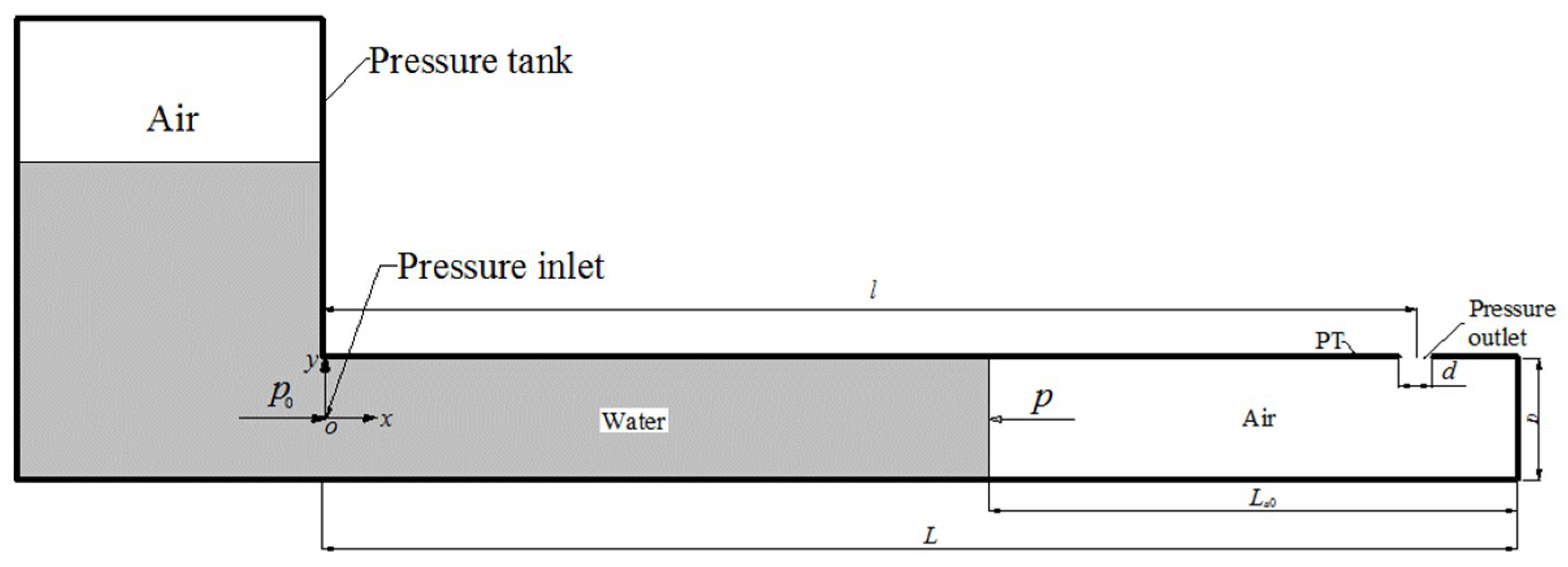
Figure 1 defines terms needed for the linearized analytical model to describe the pressure transient within an air pocket entrapped at the end of a horizontal pipe during a rapid filling process. p₀ is the absolute pressure head of water at the inlet; p is the absolute pressure of an air pocket at any given time t; and L_a0 is the initial length of the air pocket. The origin (x = 0, y = 0) is selected at the center of the pipe inlet. X represents the water–air interface displacement along the x-axis, the origin of which is the initial location of air–water interface. The governing equations mainly include the ideal gas equation and the momentum equation of water. The following assumptions are made in the development of this theoretical model: (1) the water column is rigid [24]; (2) the interface is vertical during the filling process [2]; (3) a polytropic law is applicable for the air phase [2,17,23]; (4) the head loss caused by the wall friction is neglected; (5) the air pocket has no flow resistance inertia and thus a constant pressure throughout; and (6) the flow in the pipe can be approximated as one-dimensional.

Based on the above assumptions, the motion equation of the water column in x direction can be written as

$$\rho \left(L-L_{a0}+X\right)\frac{d^{2}X}{d{t}^2}=p_0-p$$

(1)

where L is the length of the pipe, ρ is the density of water, and g is gravitational acceleration. The ideal gas equation is

$$p{V}_a^k=c$$

(2)

where V_a is the volume of the air pocket, c is a constant, and k is the polytropic exponent. According to suggestions by Lee [17], we assumed that k = 1.4 in this study. If there is no air leakage (i.e., d = 0 in Figure 1) from the pipe, the following equation can be obtained by taking the derivative of Equation (2) with respect to time t:

$$\frac{dp}{dt}=-k\frac{p}{V_a}\frac{d{V}_a}{dt}$$

(3)

where V_a = (L_a0 – X) × A (A is the cross-sectional area of the pipe). If t is very close to zero, p on the right side of Equation (3) can be approximately regarded as p₀. Therefore, Equation (3) can be rewritten as

$$\frac{dp}{dt}=k\frac{p_0}{L_{a0}-X}\frac{dX}{dt}$$

(4)

Taking the derivative with respect to time t on both sides of Equation (4), it becomes

$$\frac{d^{2}p}{d{t}^2}=k\frac{p_0}{L_{a0}-X}\frac{d^{2}X}{d{t}^2}$$

(5)

Combining Equations (1) and (5) gives

$$\rho \left(L-L_{a0}+X\right)\frac{L_{a0}-X}{k{p}_0}\frac{d^{2}p}{d{t}^2}+p-p_0=0$$

(6)

It is assumed that the initial pressure of the air pocket is of atmospheric pressure p_a. The initial conditions of Equation (6) are: t = 0, p = p_a, dp/dt = 0. Based on the initial conditions, the analytical solution of p of Equation (6) is expressed as

$$p=\left(p_a-p_0\right)\cos \left(\sqrt{\frac{k{p}_0}{\rho \left(L-L_{a0}+X\right)\left(L_{a0}-X\right)}}·t\right)+p_0$$

(7)

From Equation (7), the transient pressure caused by the entrapped air pocket is a mathematical function similar to a sine wave that describes a smooth repetitive oscillation with time. Both the oscillation period and the time when the pressure reaches its first peak (t_p) are dependent on X.

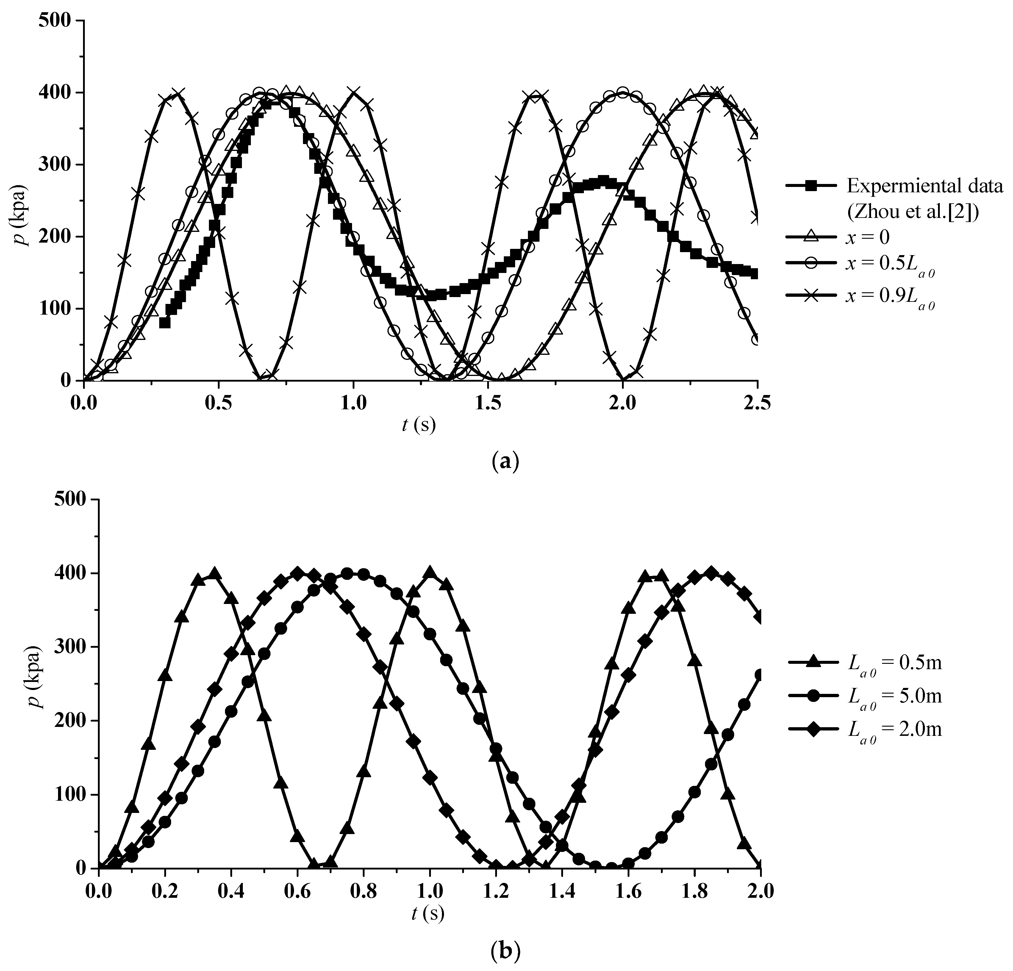
The experiments of Zhou et al. [2] are used to validate the analytical model of p. In their study, the length of the pipe, L, was 10 m and the inside diameter D was 35 mm. One scenario of Zhou et al. [2] was selected, in which p₀ = 304 kPa (relative pressure p = 206 kPa), L_a0 = 5 m, k = 1.4, p_a = 98 kPa. These values were taken into Equation (7) to solve the transient pressure within an air pocket trapped at the end of a horizontal pipe with a dead end. In order to compare with the experimental data of Zhou et al. [2], the solutions from Equation (7) are transformed into relative pressure instead of absolute pressure head. The comparison between the analytical solution and experimental data is shown in Figure 2a. The influence of the air–water interface displacement X, as an implicit function of time t on p, is also presented, where X is taken as 0, 0.5L_a0 and 0.9L_a0. Equation (7) indicates that the maximum p is about two times that of the inlet pressure. The inlet pressure and initial length of air pocket have significant influences on the amplitude of the oscillation period and t_p. It is confirmed by the experimental observations [2,18,19] and numerical simulation in our previous study [23] that the oscillation period increases along with the initial length of the air pocket and decreases as the inlet pressure increases, as shown in Figure 2b. Additionally, from Equation (7), the impact of varying the initial length of the air pocket on the amplitude of the maximum pressure is negligible. This result is consistent with Zhou et al. [2]. In one scenario, where p₀ = 336 kPa in their study, when the L_a0/L was equal to 0.048, 0.5, 0.8, the corresponding maximum pressure for each L_a0/L was 1.5, 1.6, 2.1 times the inlet pressure, respectively, which indicated that the initial length of the air pocket had a limited effect on the maximum pressure.

From Figure 2a, if X = 0, the relative differences between the analytical and experimental data at the maximum pressure, the moment when the peak pressure occurs (t_p) and the oscillation period are 2.5%, 7.1% and 21%, respectively. Taking X = 0.5L_a0, the differences are 2.5%, 13%, 2%, respectively, while if X = 0.9L_a0, they are 2.5%, 50%, and 50%, respectively. The results indicate that the analytical solutions for the maximum pressure and oscillation period with Equation (7) where X is adopted as 0.5L_a0 fit best with the experimental data. The difference is mainly due to the model assumptions given above. Note that the oscillation magnitude of the analytical solution is not damped due to neglecting the friction term in Equation (2). Therefore, Equation (7) actually provides the possible maximum pressure caused by the entrapped air pocket during the rapid filling process. In practice, the maximum pressure and oscillation frequency are the main safety concerns for pipelines. Therefore, the equation can be used for an approximate estimation for the possible pressure peak of such a system. It is worth mentioning that the analytical model deals with the cases with no ventilation or negligible air release. For these ideal cases, analytical solutions provide general guidance on the behavior of the pressure variations. For cases with notable air release, the nonlinearity of the problem and the non-conservation of the system require models which incorporate principles of airflow through the orifice and waterhammer equations. The above analytical model fails and the CFD model needs to be introduced for such scenarios.

3. Numerical Model Setup and Validation

To examine the influence of a vent location on pressure transients caused by entrapped air and its release, it is important to gain a full understanding of the detailed flow process associated with air pressurization and expulsion development. To this end, the commercially available CFD software, ANSYS Fluent (ANSYS, Canonsburg, PA, USA), was employed in this study to solve the conservation of mass and momentum equations for the specified model setup as shown in Figure 1. The volume of fluid (VOF) method and the standard k-ε turbulence model were used.

In the simulation, the air vent was simplified into an orifice placed at the pipe crown (Figure 1). The setup of the orifice diameter (d = 7 mm) and pipe size (D = 35 mm) used in Zhou et al. [2] is adopted in this study; i.e., the diameter ratio (d/D) is 0.2. Eight cases were simulated with l* = 0.00045, 0.4, 0.5, 0.6, 0.75, 0.85, 0.93 and 0.99, where l* = l/L with l being the distance from the inlet to the center of the orifice and L being the pipe length. A monitoring point for air pocket pressure, indicated as PT in Figure 1, is located 9.30 m downstream of the inlet.

Water at 293 K is selected as one of the operating fluids, and it is assumed to be incompressible. Air is considered as an ideal gas, the initial temperature of which is set to be equal to the water. To reduce computing time, the pressure tank shown in Figure 1 was not included in the CFD model. Instead, a uniform and constant pressure of 206 kPa is defined as the boundary condition at the pipe entrance (pressure inlet indicated in Figure 1). A pressure-outlet with an atmospheric pressure value is applied to the orifice. In all cases, the pipe walls are set as non-slip, and the standard wall function is used for the turbulent boundary layer in the near wall region. The solver is set up for an unsteady state. The initial air pressure is set as atmospheric, the initial velocity of water column is zero and the initial interface is vertical. All the simulations are started with an initial length of the air pocket of 5.0 m.

The simulation domain is divided into discrete control volumes by the structured grid. The robust pressure implicit with splitting of operators (PISO) method is employed to accomplish the coupling solution of velocity and pressure equations. In the experiments of Zhou et al. [2] which we used for our model validation and comparison, the reported experimental time varied from 2.0 s to 3.5 s for different experimental setups. In this study, we followed these results with simulation times which varied from 2.2 s to 3.5 s, and the time step was set as 10⁻⁵ s. The peak pressure and oscillation period were chosen as the objectives to test the mesh independence. Local refinement for the air part (the mesh size ratio of the water part to the air part was about 1.4) was used for the grid. The minimum and maximum volume of the mesh were 6.78 × 10⁻¹⁰ m³ and 2.48 × 10⁻⁸ m³, respectively. By comparing the results with different mesh resolutions, little difference is found by using a finer mesh size when the node number reached about 900,000. Therefore, the group of unstructured meshes with about 956,000 elements is used in this study to ensure both computational efficiency and accuracy.

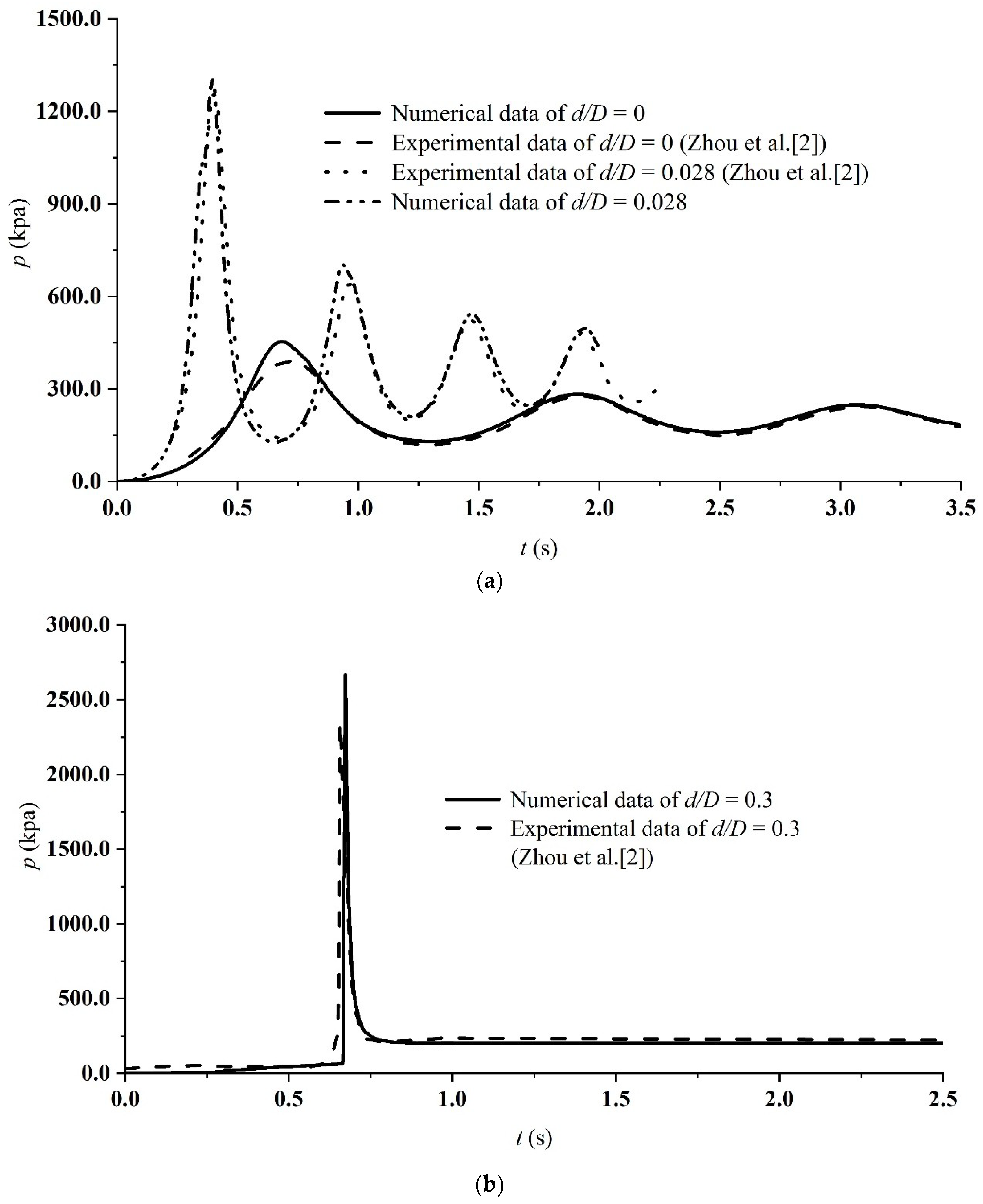
The experimental results of Zhou et al. [2] were used to validate the numerical model for the three cases with d/D = 0, 0.028, 0.3. It can be clearly seen in Figure 3 that the simulated pressure patterns are in good agreement with the experimental data. The simulated peak pressures are slightly greater than the experimental results because the wall was considered as rigid in the simulation.

4. Results and Discussion

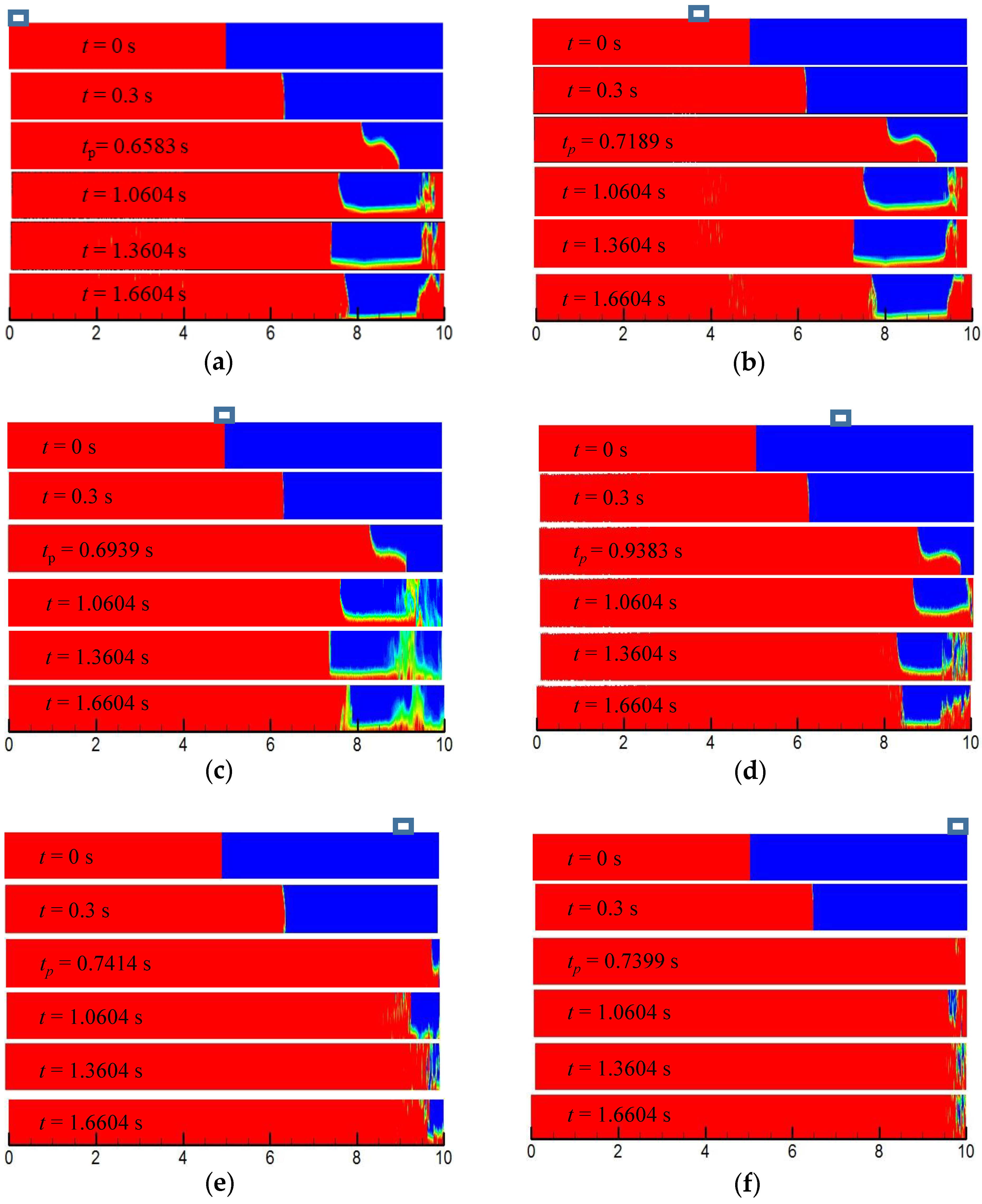
In order to understand the detailed flow processes associated with air pressurization and release through an orifice at different positions, the simulation results of some selected cases are shown in Figure 4, Figure 5, Figure 6, Figure 7, Figure 8 and Figure 9. The volume fractions of the air phase at the centerline profile at different times for l* = 0.00045, 0.4, 0.5, 0.75, 0.93 and 0.99 are shown in Figure 4 to illustrate the air–water movements over the transient process. The red color is for air pockets (the volume fraction α = 1) and the blue for water (α = 0). The same time steps are selected for comparison with each other, except the moment t_p when the maximum pressure is attained. The time t_p varies for different cases due to the influence of the venting location. For l* = 0.4, when t is between 0 and t_p, water starts flowing towards the downstream end driven by the inlet pressure. Since the orifice is blocked by water all the time, the air is kept pressurized instead of escaping from the pipe. At t_p = 0.7189 s, its length is only about 2.0 m, which is about 40% of the initial value. After t_p, the length of air pocket is longer than that at t_p and the air pocket begins to expand. For l* <= 0.5, the air pocket experiences a similar process of compression and expansion as no air can be released. The lengths of the residual air pocket at t_p for the cases of l* <= 0.5 are very close to each other, which means the volume of residual air has not been influenced by the location of air ventilation. For l* = 0.75, t_p registers the largest value compared to other cases. The filling process consists of two stages, namely air venting before the water column reaches the orifice and air compression afterwards. For those cases (l* <= 0.75), the water column has not yet arrived at the end of the pipe when the peak surge pressure occurs; as a result, the air pocket still occupies the entire cross section.

For l* = 0.99 (see Figure 4f), the water arrives at the end of the pipe much more quickly than that for the other cases, as most of the initial air pocket is almost vented through the outlet. At t_p = 0.7399 s, the water column slams on the pipe end wall. After that, the pipe is nearly filled with the water phase. The variations of the length of the air pockets with time for l* = 0.93 and 0.85 are similar to the case of l* = 0.99, but the volume of the residual air pocket after t_p is smaller as l* increases. For example, the corresponding volume fractions of the residual air pocket to l* = 0.85, 0.93 and 0.99 are 15%, 8%, 2%, respectively.

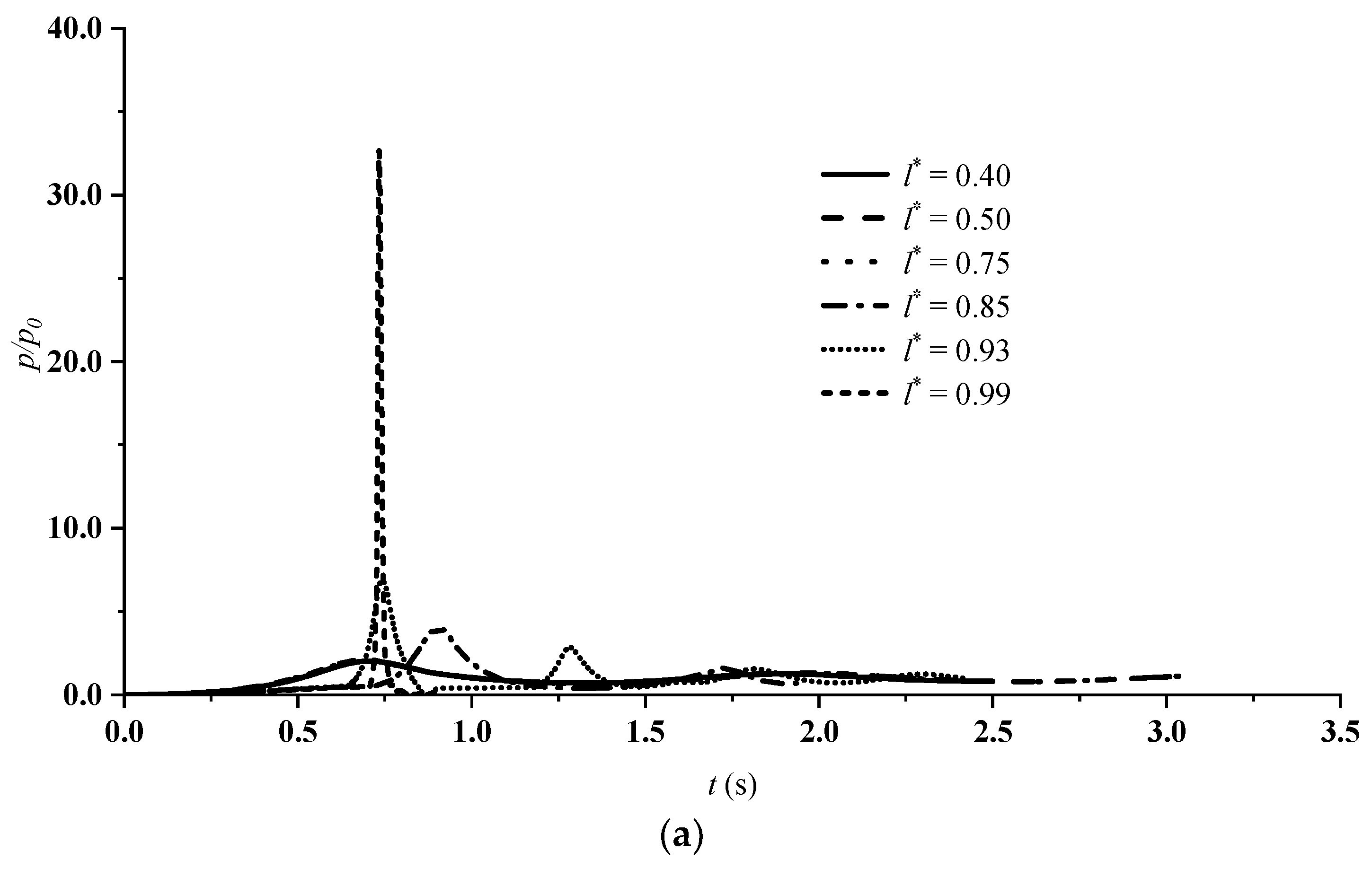
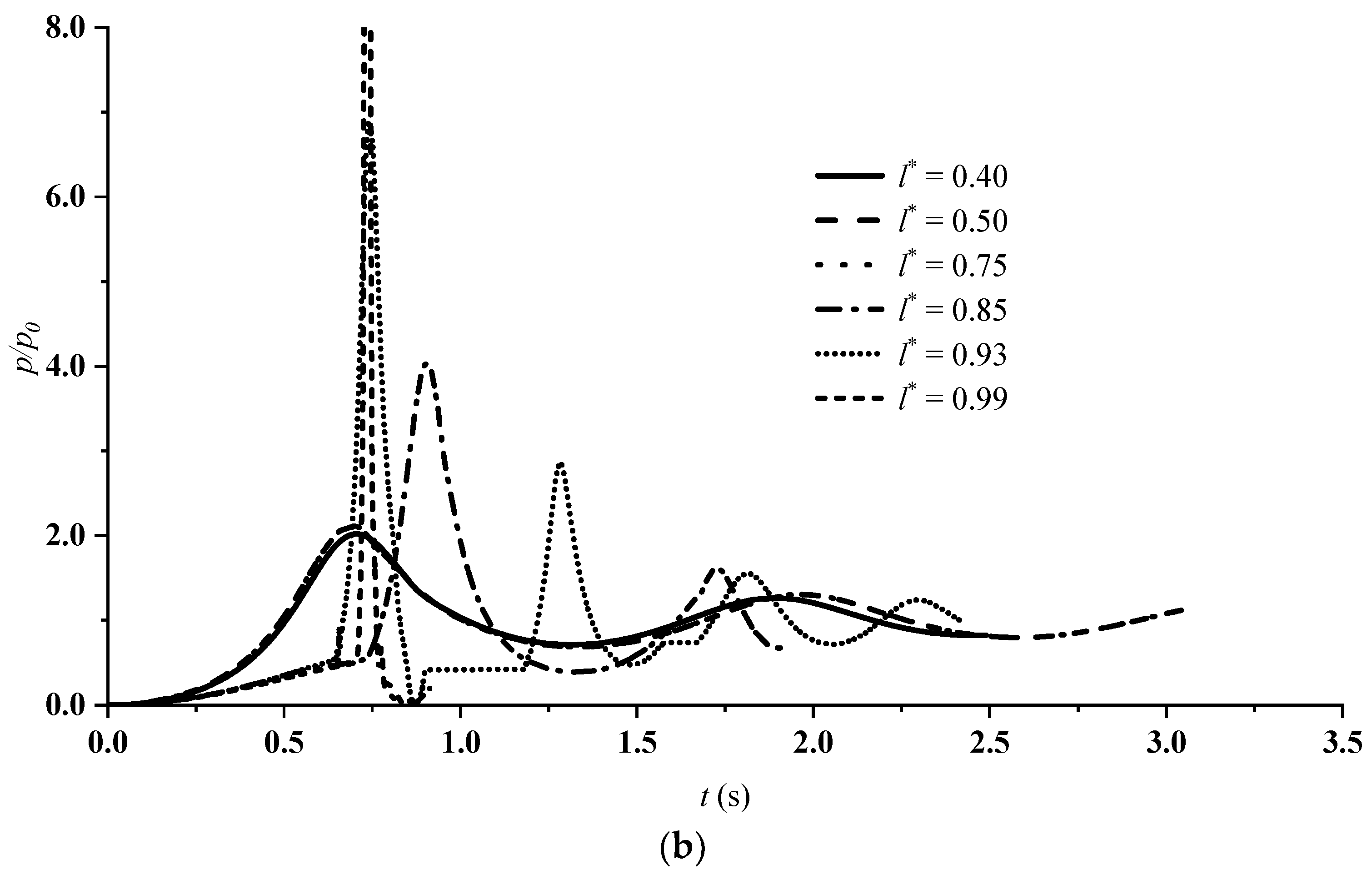
The simulated pressure oscillations for all cases are examined, and it is found that there are primarily two types of behavior depending on the location of the leakage orifice, as shown in Figure 5, which is similar to the results of the pipe with an end orifice [2]. For l* < 0.99, the pressure variation is dominated by the long or short period oscillation and dampened by the air pocket as the initial air may not be released or only a part of it may be released after the initiation of water column movement; whereas for l* = 0.99, there is no sign of pressure oscillation. Instead, only waterhammer-like pressure is observed.

The variations of air pressure over time for the cases of l* = 0.00045, 0.4, 0.5 are almost identical (see Figure 5 (the line for l* = 0.00045 is not listed due to the overlap of the three lines)). In these cases, an orifice is located in the section of the water column, and leakage volume of the initial air pocket is almost zero. Before t_p, the increasing rates of air pressure are greater than that of other cases, which means that the compression rate of the air pocket is greater. It takes a shorter time to attain the peak value (t_p = 0.7189 s), 400 kPa, which is about 2 times the driving pressure (p₀ = 206 kPa) at the pipe entrance. After t_p, the pressure decreases over time as air pocket expands. The air pressure oscillates with decaying peak magnitudes, primarily due to the cushion effect of the air pocket and friction damping. When a very small part of the air is released from the orifice, such as for the case of l* = 0.5 or 0.6, which is similar to that of l* < 0.6, most of the initial air pocket is prevented from escaping due to the water column blocking the orifice soon after t > 0. Therefore, the maximum pressure and oscillation period are almost the same as that for l* < 0.6.

For l* = 0.75, more than 30% of the initial air volume has been released before the water column arrives at the cross section where the orifice is located. Compared to the cases of l* < 0.75, since part of the kinetic energy of the water column is converted into the kinetic energy of the released air, and the rest of the kinetic energy is then converted into the potential energy of the air pocket, the maximum pressure is about 1.6 times the smaller inlet pressure. It takes more time to reach the peak pressure than for other cases. Meanwhile, due to the cushion and damping effect, the transient pressure still oscillates, but the oscillation period is shorter than that for l* < 0.75 because of the smaller volume of residual air.

When l* increases from 0.75 to 0.93, the maximum pressure increases from 1.6 times to 7 times the inlet pressure, and the oscillation period decreases significantly. The reason for this is that the pressure variation for both l* = 0.93 or 0.99 is gradually dominated by the waterhammer effect instead of air compression and expansion due to lower effect of the air cushion than for l* < 0.93. The volume ratio of the residual air to the initial value at t_p for l* = 0.75, 0.85 and 0.93 is 17.5%, 9.2%, 2.3%, respectively. When l* increases to 0.99, the residual air is only 0.08% of the initial volume and the air cushion effect is negligible. At t_p, the water impinges directly on the pipe end, and the pressure increases suddenly to its peak value which is about 30 times the inlet pressure. For a case in Zhou et al. [2] with an inlet pressure of 206 kPa and an initial length of the air pocket of 5 m, the peak pressure is 32 times the inlet pressure in a pipe with an end orifice of the same diameter as that in this study. This means that once waterhammer happens, the waterhammer pressure is independent of the specific location of the orifice. After t_p, the pressure drops to a constant value as the pipe is filled with water.

Referring to Figure 4 and Figure 5, it can be concluded that the location of the air vent directly influences the types of pressure oscillation and peak values which are mainly related to the volume of the residual air when the water flow arrives at the end of the pipe.

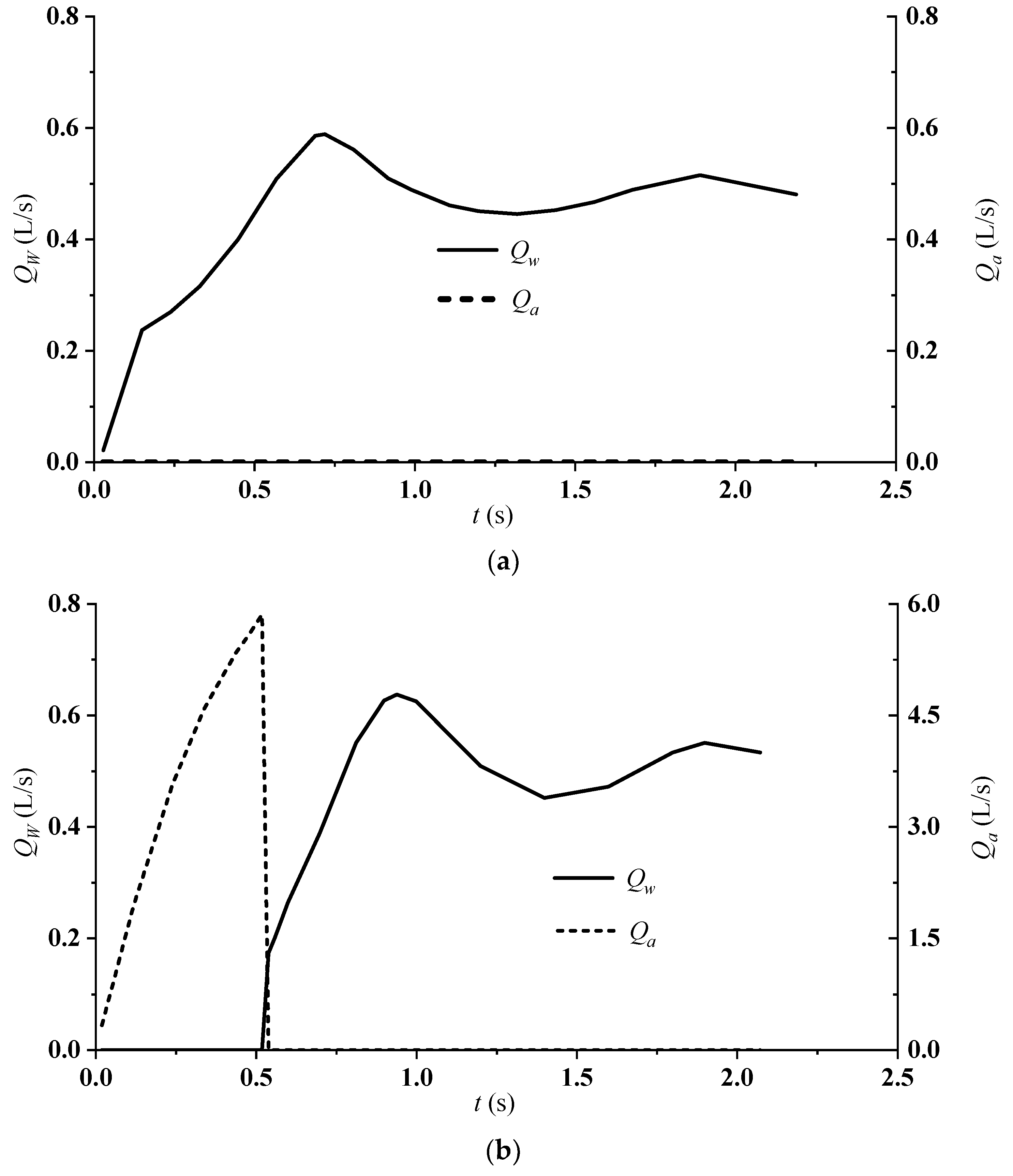
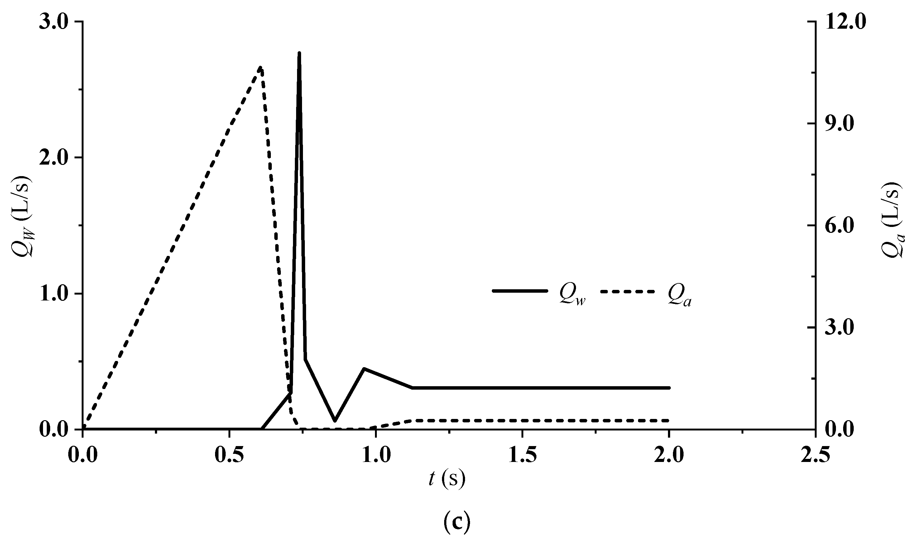
Figure 6 shows the variation of the flow rate of water and air (Q_w, Q_a) vented from the orifice with time for several typical cases. From Figure 6a, for l* = 0.4, Q_a is zero throughout the filling process because of water blocking off the orifice to prevent the air from escaping. The variation of Q_w with time is the same as that of the pressure. At t_p = 0.7089 s, Q_w reaches its maximum at 0.6 L/s when the pressure is at its peak value. The decrease of pressure causes Q_w to decrease. For l* = 0.75 (Figure 6b), since the orifice is installed within the middle of the initial air pocket, from the initiation, Q_a proportionally increases with time and Q_w is zero. At t = 0.5 s, Q_a reaches its peak value at 6 L/s. After that, Q_a drops rapidly to zero due to the arrival of water, and Q_w increases suddenly, then it varies with time as pressure does. The peak value of Q_w is very close to that for l* = 0.4, but the time when Q_w obtains its first peak increases as l*. From Figure 6c, since the location of an orifice is very near the end of the air pocket, almost all the air driven by the inlet pressure is exhausted. Q_a increases more quickly than that in the cases of l* = 0.4 and 0.75 as the kinetic energy of water column is converted into energy of orifice flow. At t = 0.6 s, Q_a attains its peak value 10.74 L/s. After that, Q_a drops rapidly and Q_w increases from zero to 0.5 L/s since the bottom of the water column has arrived at the pipe end and water occupies the cross section of orifice suddenly. At t_p = 0.7399 s, Q_w obtains its peak value 2.8 L/s. Q_w is 4 times that for l* = 0.75 and 0.4 since the peak pressure of l* = 0.99 is 16 times that for l* = 0.75 and 0.4, which indicates that the orifice flow rate is proportional to the square root of the pressure head. After t_p, Q_w drops to a constant value as the water has filled the pipe.

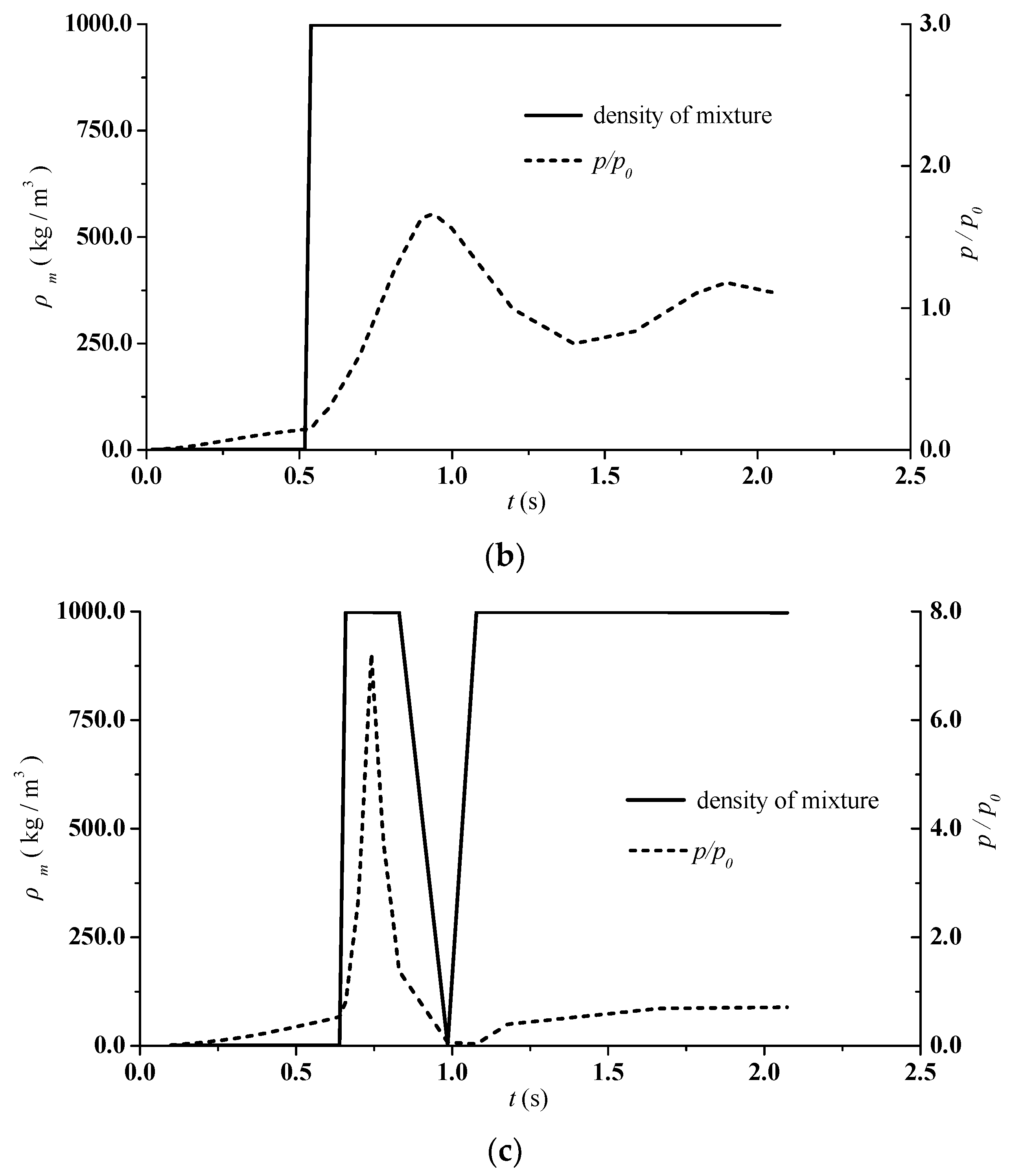
Figure 7 shows the relation between the density of the air–water mixture, ρ_m, through the outlet and air pocket pressure for different cases. From Figure 7a, for l* = 0.4, when the pressure attains the first peak value, ρ_m is about 998 kg/m³ since the mixture is only consisted of water. After t_p, the density oscillates with time since the air pockets expand and flow toward to the outlet with water. The smallest density of the mixture is about 975 kg/m³ when the pressure obtains its first trough. The variation of density for l* = 0.75 is not similar to that for l* = 0.4 although pressure patterns in the two cases are similar. From 0 to 0.5 s, ρ_m increases from 1.22 kg/m³ (air density) quickly to 998 kg/m³ (water density). During the filling process, there is no mixture of water and air from the orifice. At t_p, ρ_m is 998 kg/m³. For l* = 0.93, before and after t_p, the density is about 998 kg/m³ which means the length of the air pocket is less than 0.07 m. From 0.83 to 0.99 s, ρ_m drops to the density of air since the air pocket expands toward to the orifice and occupies the cross section of the orifice. After that, ρ_m increases to 998 kg/m³ instantly since the residual air pocket keeps being vented and the volume of air pocket decreases.

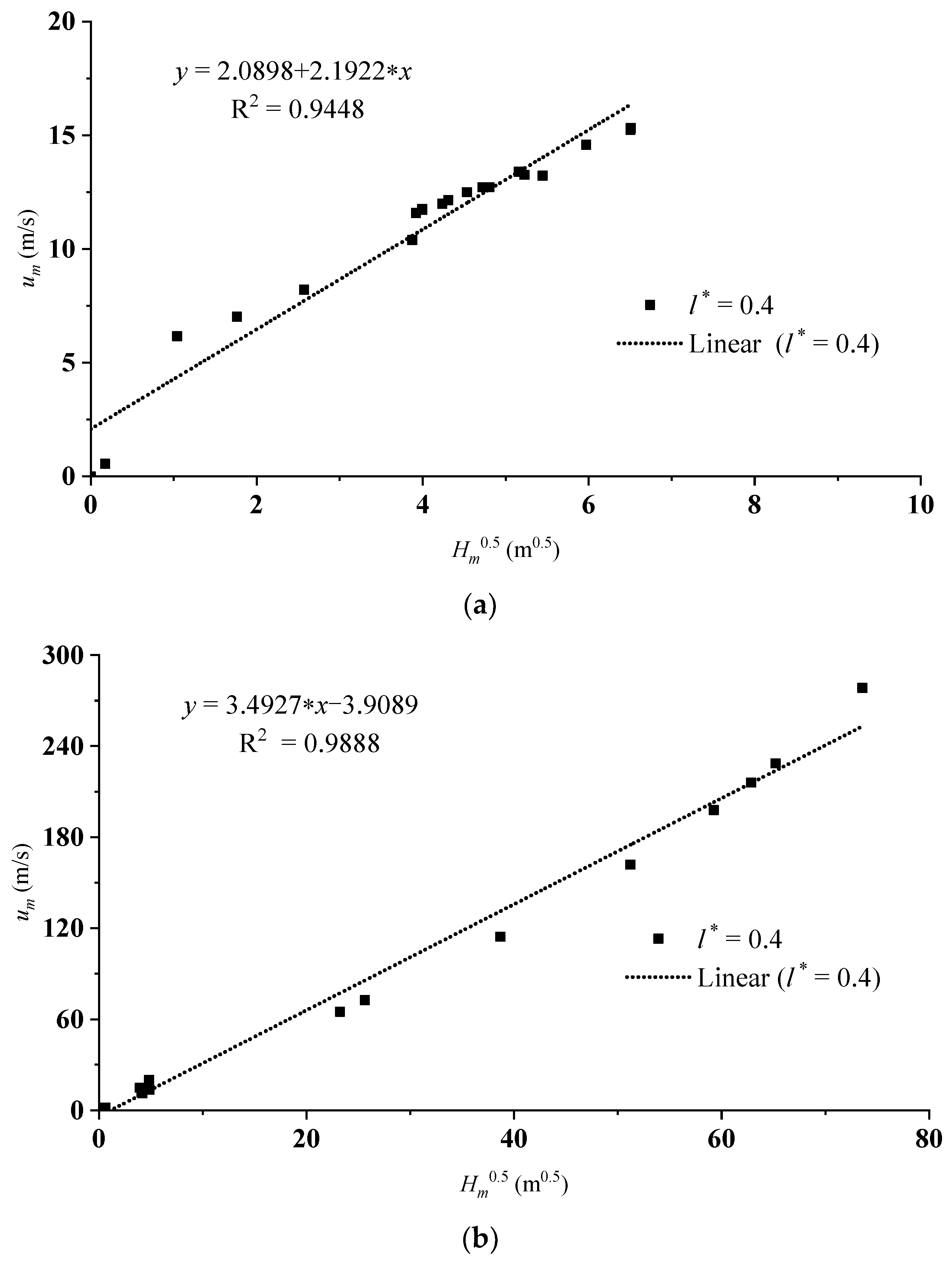
In order to clarify the relation between the pressure head H_m and average velocity u_m of the mixture at the orifice, variations of H_m^0.5 and u_m with time for some selected cases are shown in Figure 8, where H_m and u_m are expressed as Equations (8) and (9), respectively. Referring to Figure 8, both have very similar variations.

$$H_m\left(t\right)=\frac{p\left(t\right)}{{\rho }_m\left(t\right)g}$$

(8)

$$u_m\left(t\right)=\frac{Q_a\left(t\right)+Q_w\left(t\right)}{A_o}$$

(9)

where A_o = the cross-section area of the orifice.

The relationship between H_m^0.5 and u_m for l* = 0.4 and 0.99 at different times were analyzed and are presented in Figure 9. It can be seen that u_m increases linearly with H_m^0.5 for both cases. The velocity of the mixture u_m out of the orifice increases linearly with H_m^0.5 (H_m: the driving head) for the cases under study, which indicates that the energy relationship can be applied to such an air–water flow system under unsteady conditions.

5. Conclusions

Air–water actions lead to many problems, including pressure transients and geysering, for a pipe system when filling or emptying. In this paper, a simple analytical model was developed for predicting the maximum pressure and oscillation period of transient pressure for a rapid-filling pipe with trapped air. The analytical model was validated using previous laboratory measurements. It can be easily used to estimate the pressure pattern of a confined system with entrapped air or when very poor ventilation exists, instead of the numerical computing of a system of nonlinear equations. The analytical model suggests that the transient pressure is a mathematical function similar to a sine wave that describes a smooth repetitive oscillation with time. The peak pressure is about two times the inlet pressure, and the oscillation period increases with the initial length of the air pocket and decreases with the increase of the inlet pressure. The inlet pressure and initial length of the air pocket have significant influences on the amplitude of the oscillation period and the time to reach the peak pressure, t_p. The initial length of the air pocket has a negligible effect on the peak pressure.

When the pipeline has air vents through which the trapped air can escape, water slamming arises under certain conditions. A 3D CFD model was applied to simulate the water–air-flow process for a rapidly filling pipe. The air–water interface cannot remain vertical due to gravity, and the pressure rise of the air pocket contributes to the deformation of the interface and the generation of air–water mixture, which are beyond the ability of all of 1D analytical/numerical models. The influence of the venting location, represented by a parameter l* (a ratio of the distance from the inlet to the center of the orifice to the pipe length), on transient behaviors was elucidated. For the study cases, there are mainly two types of pressure oscillation patterns, namely long or short-period oscillations and waterhammer-like behavior. The differences between them are due to the variation of volume fractions of residual air with regard to time, dependent on the location of the orifice. Variations of the flow rate of water or air and the density of the air–water mixture through the top orifice are different with regard to l*. The three-dimensional CFD model, while losing its generality, provides significant details regarding the hydrodynamics of the air–water flow and enhances our understanding of the rapid-filling process. These findings should be helpful to guide the design of air vents for pipeline networks and sewer systems. Future studies will involve mathematical models for cases with air leakage and investigate air–water interactions in stormwater sewer systems, such as geysering through vertical structures.

References

- Tijsseling, A.; Hou, Q.; Bozkuş, Z.; Laanearu, J. Improved one-dimensional models for rapid emptying and filling of pipelines. J. Press. Vessel Technol. 2016, 138, 031301. [Google Scholar] [CrossRef]
- Zhou, F.; Hicks, F.; Steffler, P. Transient flow in a rapidly filling horizontal pipe containing trapped air. J. Hydraul. Eng. 2002, 128, 625–634. [Google Scholar] [CrossRef]
- Zhou, F.; Hicks, F.; Steffler, P. Analysis of effects of air pocket on hydraulic failure of urban drainage infrastructure. Can. J. Civ. Eng. 2004, 31, 86–94. [Google Scholar] [CrossRef]
- Zhou, L.; Liu, D.; Karney, B. Investigation of hydraulic transients of two entrapped air pockets in a water pipeline. J. Hydraul. Eng. 2013, 139, 949–959. [Google Scholar] [CrossRef]
- Zhou, L.; Liu, D.; Karney, B.; Zhang, Q. Influence of entrapped air pockets on hydraulic transients in water pipelines. J. Hydraul. Eng. 2011, 137, 1686–1692. [Google Scholar] [CrossRef]
- Fuertes-Miquel, V.S.; Coronado-Hernández, O.E.; Iglesias-Rey, P.L.; Mora-Melia, D. Transient phenomena during the emptying process of a single pipe with water–air interaction. J. Hydraul. Res. 2018. [Google Scholar] [CrossRef]
- Coronado-Hernández, O.E.; Fuertes-Miquel, V.S.; Besharat, M.; Ramos, H.M. Experimental and numerical analysis of a water emptying pipeline using different air valves. Water 2017, 9, 98. [Google Scholar] [CrossRef]
- Laanearu, J.; Annus, I.; Koppel, T.; Bergant, A.; Vuckovic, S.; Hou, Q.; Tijsseling, A.; Anderson, A.; Van’t Westende, J. Emptying of large-scale pipeline by pressurized air. J. Hydraul. Eng. 2012, 138, 1090–1100. [Google Scholar] [CrossRef]
- Balacco, G.; Apollonio, C.; Piccinni, A.F. Experimental analysis of air valve behaviour during hydraulic transients. J. Appl. Water Eng. Res. 2015, 3, 3–11. [Google Scholar] [CrossRef]
- Li, J.; McCorquodale, A. Modeling mixed flow in storm sewers. J. Hydraul. Eng. 1999, 125, 1170–1180. [Google Scholar] [CrossRef]
- Wright, S.J.; Lewis, J.W.; Vasconcelos, J.G. Geysering in rapidly filling storm-water tunnels. J. Hydraul. Eng. 2010, 137, 112–115. [Google Scholar] [CrossRef]
- Guo, Q.; Song, C.C. Surging in urban storm drainage systems. J. Hydraul. Eng. 1990, 116, 1523–1537. [Google Scholar] [CrossRef]
- Guo, Q.; Song, C.C. Dropshaft hydrodynamics under transient conditions. J. Hydraul. Eng. 1991, 117, 1042–1055. [Google Scholar] [CrossRef]
- Wright, S.J.; Lewis, J.W.; Vasconcelos, J.G. Physical processes resulting in geysers in rapidly filling storm-water tunnels. J. Irrig. Drain. Eng. 2011, 137, 199–202. [Google Scholar] [CrossRef]
- Cong, J.; Chan, S.N.; Lee, J.H.W. Geyser formation by release of entrapped air from horizontal pipe into vertical shaft. J. Hydraul. Eng. 2017, 143. [Google Scholar] [CrossRef]
- Huang, B.; Wu, S.; Zhu, D.Z.; Schulz, H.E. Experimental study of geysers through a vent pipe connected to flowing sewers. Water Sci. Technol. 2018, 2017, 66–76. [Google Scholar] [CrossRef] [PubMed]
- Lee, N.H. Effect of Pressurization and Expulsion of Entrapped Air in Pipelines. PhD Thesis, Georgia Institute of Technology, Atlanta, GA, USA, 2005. [Google Scholar]
- De Martino, G.; Fontana, N.; Giugni, M. Transient flow caused by air expulsion through an orifice. J. Hydraul. Eng. 2008, 134, 1395–1399. [Google Scholar] [CrossRef]
- Bucur, D.M.; Dunca, G.; Cervantes, M.J. Maximum pressure evaluation during expulsion of entrapped air from pressurized pipelines. J. Appl. Fluid Mech. 2017, 10, 11–20. [Google Scholar] [CrossRef]
- Vasconcelos, J.G.; Wright, S.J. Experimental investigation of surges in a stormwater storage tunnel. J. Hydraul. Eng. 2005, 131, 853–861. [Google Scholar] [CrossRef]
- Zhou, L.; Wang, H.; Karney, B.; Liu, D.; Wang, P.; Guo, S. Dynamic behavior of entrapped air pocket in a water filling pipeline. J. Hydraul. Eng. 2018, 144. [Google Scholar] [CrossRef]
- Apollonio, C.; Balacco, G.; Fontana, N.; Giugni, M.; Marini, G.; Piccinni, A. F. Hydraulic transients caused by air expulsion during rapid filling of undulating pipelines. Water 2016, 8, 25. [Google Scholar] [CrossRef]
- Martin, C.S. Entrapped air in pipelines. In Proceedings of the 2nd International Conference on Pressure Surges; British Hydromechanics Research Association: Bedford, UK, 1976; pp. 15–27. [Google Scholar]
- Cabrera, E.; Abreu, J.; Pérez, R.; Vela, A. Influence of liquid length variation in hydraulic transients. J. Hydraul. Eng. 1992, 118, 1639–1650. [Google Scholar] [CrossRef]
- Albertson, M.L.; Andrews, J. Transients caused by air release. In Control of Flow in Closed Conduits; Colorado State University: Fort Collins, CO, USA, 1971; pp. 315–340. [Google Scholar]
- Catano-Lopera, Y.A.; Tokyay, T.E.; Martin, J.E.; Schmidt, A.R.; Lanyon, R.; Fitzpatrick, K.; Scalise, C.; Garcia, M.H. Modeling of a transient event in the tunnel and reservoir plan system in chicago, illinois. J. Hydraul. Eng. 2014, 140, 05014005. [Google Scholar] [CrossRef]
- Zhou, L.; Liu, D.; Ou, C. Simulation of flow transients in a water filling pipe containing entrapped air pocket with VOF model. Eng. Appl. Comput. Fluid Mech. 2011, 5, 127–140. [Google Scholar] [CrossRef]
- Li, L.; Zhu, D.Z. Modulation of transient pressure by an air pocket in a horizontal pipe with an end orifice. Water Sci. Technol. 2018, 77, 2528–2536. [Google Scholar] [CrossRef] [PubMed]
- Martins, N.M.C.; Soares, A.K.; Ramos, H.M.; Covas, D.I.C. CFD modeling of transient flow in pressurized pipes. Comput. Fluids 2016, 126, 129–140. [Google Scholar] [CrossRef]
- Martins, N.M.C.; Delgado, J.N.; Ramos, H.M.; Covas, D.I.C. Maximum transient pressures in a rapidly filling pipeline with entrapped air using a CFD model. J. Hydraul. Res. 2017, 55, 506–519. [Google Scholar] [CrossRef]
Figure 1.
Schematic and boundary conditions of a pressurized horizontal pipe system containing entrapped air (l = the distance between the pipe entrance and the venting orifice; d = the diameter of the venting orifice; D = pipe diameter; PT = pressure transducer).
Figure 2.
Variation of the air pressure with time: (a) Comparison between the analytical solution and experimental data in Zhou et al. [2] (La0/L = 0.5, k = 1.4, relative pressure p0 = 206 kPa); (b) Effect of different initial length of the air pocket (k = 1.4, relative pressure p0 = 206 kPa, and X in Equation (7) is equal to zero).
Figure 3.
Comparison of pressure variation between the simulations in this study and experimental measurements of Zhou et al. [2] for different orifice sizes (a) d/D = 0 and d/D = 0.028; (b) d/D = 0.3.
Figure 4.
Evolution of the entrapped air on the vertical center plane for (a) l* = 0.00045; (b) l* = 0.40; (c) l* = 0.50; (d) l* = 0.75; (e) l* = 0.93; (f) l*= 0.99. Note: tp represents the time when the pressure attains the maximum value; the red color indicates the air phase and the blue is for water. The rectangle at the top side of the pipe represents the venting orifice.
Figure 5.
Pressure signatures at the pressure transducer (PT) for various l*: (a) Overview; (b) Details.
Figure 6.
Variation of air–water flow rates through the orifice with time for (a) l* = 0.4; (b) l* = 0.75; (c) l* = 0.99.
Figure 7.
Variation of the mixture density at the orifice and the pressure at PT with time for (a) l* = 0.4; (b) l* = 0.75; (c) l* = 0.99.
Figure 8.
Variation of the air pressure head and mixture velocity at the orifice for (a) l* = 0.4; (b) l* = 0.75; (c) l* = 0.99.
Figure 9.
Relationship between the air pressure head and mixture velocity at outlet for (a) l* = 0.4; (b) l* = 0.99.
© 2018 by the authors. Licensee MDPI, Basel, Switzerland. This article is an open access article distributed under the terms and conditions of the Creative Commons Attribution (CC BY) license (http://creativecommons.org/licenses/by/4.0/).
Share and Cite
MDPI and ACS Style
Li, L.; Zhu, D.Z.; Huang, B. Analysis of Pressure Transient Following Rapid Filling of a Vented Horizontal Pipe. Water 2018, 10, 1698. https://doi.org/10.3390/w10111698
AMA Style
Li L, Zhu DZ, Huang B. Analysis of Pressure Transient Following Rapid Filling of a Vented Horizontal Pipe. Water. 2018; 10(11):1698. https://doi.org/10.3390/w10111698
Chicago/Turabian StyleLi, Lin, David Z. Zhu, and Biao Huang. 2018. "Analysis of Pressure Transient Following Rapid Filling of a Vented Horizontal Pipe" Water 10, no. 11: 1698. https://doi.org/10.3390/w10111698
Note that from the first issue of 2016, this journal uses article numbers instead of page numbers. See further details here.