Synthetic Impacts of Internal Climate Variability and Anthropogenic Change on Future Meteorological Droughts over China


1
State Key Laboratory of Water Resources and Hydropower Engineering Science, Wuhan University, Wuhan 430072, China
2
Department of Geosciences, University of Oslo, P.O. Box 1047 Blindern, N-0316 Oslo, Norway
*
Author to whom correspondence should be addressed.
Water 2018, 10(11), 1702; https://doi.org/10.3390/w10111702
Submission received: 18 October 2018
/
Revised: 9 November 2018
/
Accepted: 17 November 2018
/
Published: 21 November 2018
(This article belongs to the Special Issue Hydrological Impacts of Climate Change and Land Use/Land Cover Change)
Abstract
:The climate change impacts on droughts have received widespread attention in many recent studies. However, previous studies mainly attribute the changes in future droughts to human-induced climate change, while the impacts of internal climate variability (ICV) have not been addressed adequately. In order to specifically consider the ICV in drought impacts, this study investigates the changes in meteorological drought conditions for two future periods (2021–2050 and 2071–2100) relative to a historical period (1971–2000) in China, using two multi-member ensembles (MMEs). These two MMEs include a 40-member ensemble of the Community Earth System Model version 1 (CESM1) and a 10-member ensemble of the Commonwealth Scientific and Industrial Research Organization Mark, version 3.6.0 (CSIRO-Mlk3.6.0). The use of MMEs significantly increases the sample size, which makes it possible to apply an empirical distribution to drought frequency analysis. The results show that in the near future period (2021–2050), the overall drought conditions represented by drought frequency of 30- and 50-year return periods of drought duration and drought severity in China will deteriorate. More frequent droughts will occur in western China and southwestern China with longer drought duration and higher drought severity. In the far future period (2071–2100), the nationwide drought conditions will be alleviated, but model uncertainty will also become significant. Deteriorating drought conditions will continue in southwestern China over this time period. Thus, future droughts in southwestern China should be given more attention and mitigation measures need to be carefully conceived in these regions. Overall, this study proposed a method of taking into account internal climate variability in drought assessment, which is of significant importance in climate change impact studies.
1. Introduction
Drought, usually rooted in the deficiency of expected precipitation over a period of time, has received widespread attention all over the world. In contrast with aridity, which is a long-term normal climate feature in areas with low rainfall, drought is a temporary abnormal phenomenon, which is often related to human activities and can linger for years, and often causes catastrophic socio-economic and environmental consequences. Large scale drought has been observed on all continents, including Europe [1], Africa [2,3], Asia [4,5], Australia [6,7,8], and North America [9,10]. For example, from 1975 to 1976, a notorious drought caused the lowest flow on record in the majority of British rivers, loss of over 50,000 trees, and around £500 million in crop losses [11]. Therefore, an in-depth drought assessment is important for making adaption strategies.
According to the coverage, characteristic variables concerned, and developmental stages, drought has been defined in different ways and is generally classified into four categories [12,13,14]: meteorological drought, hydrological drought, agricultural drought, and socio-economic drought. Meteorological drought is defined as a lack of proper precipitation over a region for a certain time period. Hydrological, agricultural and socio-economic droughts usually follow meteorological droughts, and they generally involve specific fields such as surface water resources, soil moisture, and disparities between water demand and water supply. Apparently, as the initial stage of a drought, the meteorological drought determines the scale of a drought episode and thus is of primary importance.
Many studies have evaluated droughts spanning the meteorological drought to other categories over recent decades [15,16,17,18,19,20,21]. These studies usually involve the calculation of basic drought characteristics such as drought frequency, duration, and severity, which are combined with the theory of run [22,23,24]. For example, Xu et al. [25] utilized indices of the Standard Precipitation Index (SPI), the Reconnaissance Drought Index (RDI), and the Standard Precipitation Evapotranspiration Index (SPEI) to evaluate meteorological drought characteristics in China for 1961–2012. In addition, in order to provide more useful information on adaptation planning, drought hazards determined by return periods using frequency analysis approaches have also been analyzed in some studies [26,27,28]. For example, on the basis of the SPI, SPEI and the Composite Index (CI), Ayantobo et al. [14] estimated drought hazards over the mainland China for 1961–2013 based on a univariate frequency analysis.
In the context of global warming, drought will continue to be a dire threat in the 21st century [29,30,31]. Under the increasing concentrations of greenhouse gases (GHGs), surface temperature will increase, associated with augmenting evapotranspiration demands and changing spatial and temporal precipitation patterns. Therefore, droughts, which are derived from abnormal climatologic conditions, especially from precipitation changes, could be thereafter impacted and are expected to become more frequent and severe. For example, Sheffield et al. [29] indicated that the odds of droughts would increase due to the potential acceleration of the terrestrial water cycle under future climate change. Dai [30] showed that severe and widespread agricultural droughts would linger for the next several decades over many land areas due to climate change. Naumann et al. [31] indicated that drought conditions could worsen in many regions of the world under global warming.
However, in addition to human-induced climate change attributed to the increase in GHGs [32,33,34], internal climate variability (ICV) due to the chaotic nature of the climate system [35] is also one of the main components resulting in climate variability. ICV can strongly impact climate extremes such as droughts by superimposing on human-induced forcing [36,37,38]. For example, Trenberth et al. [39] found that the ICV could result in conflicting drought assessment results. Dai [30] also demonstrated that future drought projections would be closely related to the ICV, especially to the component of El Nino/Southern Oscillation. Orlowsky et al. [40] stated that worldwide near-term future drought changes would be in the range of ICV impacts instead of tendency changes, induced by limited anthropogenic climate change impacts.
Generally, the ICV derives from the absence of external forcing and involves processes intrinsic to the coupled system of atmosphere and ocean [41]. The time scales of the ICV range from years, decades, and multi-decades to thousands of years and even longer. Among them, the multi-decadal variability is one of the most important components in climate change impact studies, as impacts are usually assessed at a multi-decadal period (e.g., a 30-year period). In specific, the multi-decadal ICV can be investigated using long climate observations spanning hundreds to thousands of years, which is however usually not available for most regions of the world. Alternatively, the recently developed multi-member ensembles (MMEs) of a climate model [42,43,44] are specifically designed for investigating the role of ICV in climate change impacts. For example, Deser et al. [45] employed a 40-member ensemble from the Climate System Model version 3 (CCSM3) to identify the role of the ICV in future climate change in North America. These MMEs contain different members by driving the same climate model using slightly different atmospheric initial conditions and thus cover divergent climate trajectories under the same physic basis. The members in a MME embody a lot of potential possibilities of climate trajectories, while the real climate condition is expected to be a single realization among these possibilities [46]. In general, the inter-member variability, usually in the form of the range or variance of specific statistics (e.g., mean, standard variation), can manifestly represent ICV in the virtual world.
Therefore, the primary objective of this study is to investigate the synthetic impacts of ICV and anthropogenic climate change on droughts in China by using the state-of-the-art large multi-member ensembles of climate models. The synthetic impacts are specifically considered by pooling all ensemble members to estimate different levels of return periods for droughts. In addition, pooling all members of an ensemble enables using an empirical distribution to calculate the return periods for drought duration/severity, which can avoid the potential drawbacks in fitting probability distributions (e.g., great uncertainty in parameter estimation and poor extension in tails).
2. Dataset
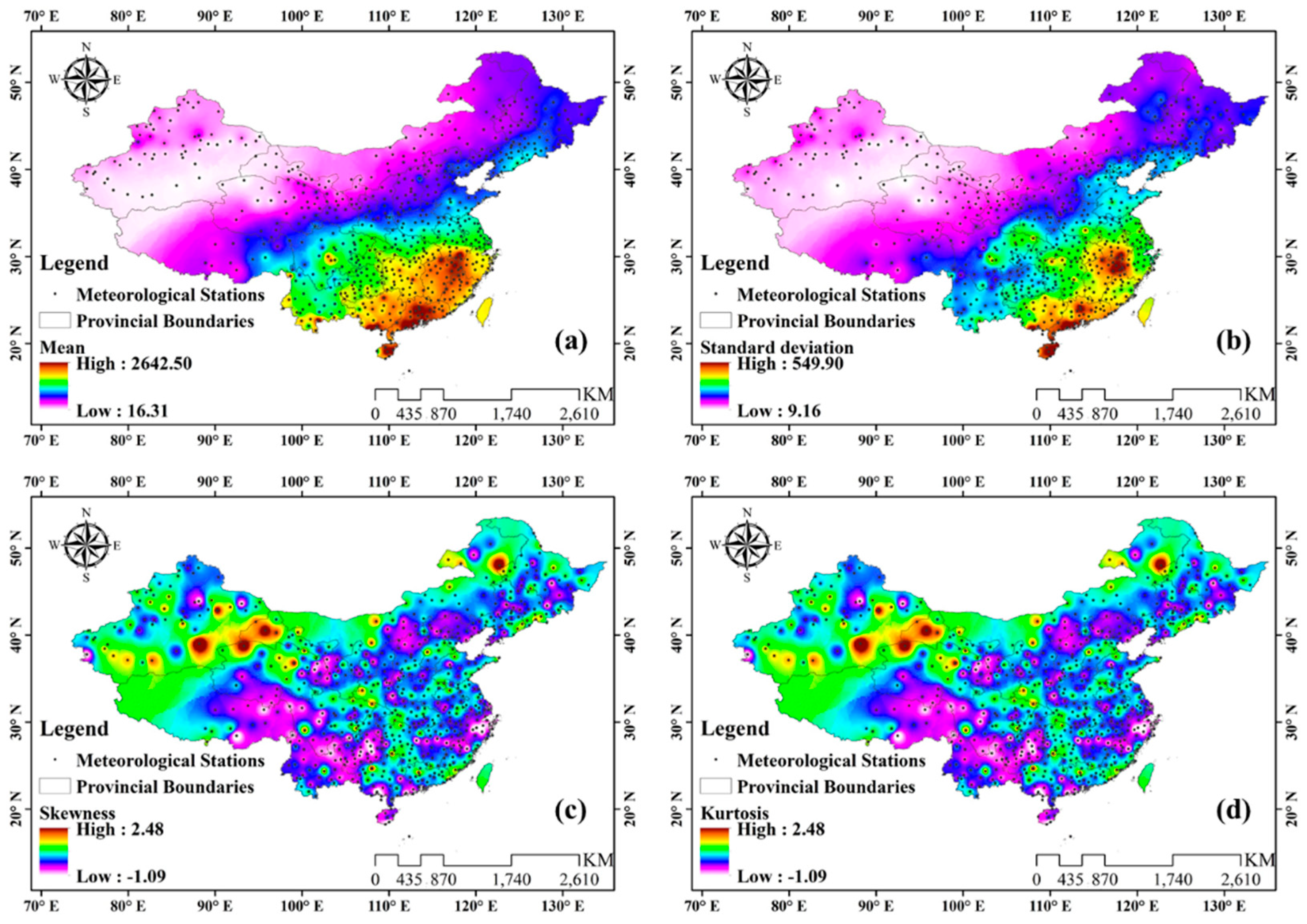
This study used both observed and climate model simulated monthly precipitation data. The observed precipitation data (OBS) were collected from 659 stations in mainland China (Figure 1) with a 30-year length for the reference baseline (1971–2000) period and provided by the China Meteorological Data Sharing Service System (http://www.cma.gov.cn). The mean, standard deviation, and skewness and kurtosis coefficients of 30-year (1971–2000) annual precipitation are presented for China. The maps of these statistics are interpolated using 659 stations. Generally, southeastern China has much more precipitation with larger variability than northwestern China. The skewness and kurtosis of annual precipitation in China tend to be scattered with higher values mainly located in northwestern China (Figure 1).
The MMEs of precipitation were extracted from two climate models: the Community Earth System Model version 1 (CESM1) (http://www.cesm.ucar.edu/projects/community-projects/LENS/data-sets.html) and the Commonwealth Scientific and Industrial Research Organization Mark, version 3.6.0 (CSIRO) (http://cmip-pcmdi.llnl.gov/cmip5). These two MMEs were selected according to their differences in model structures and the number of ensemble members. CESM1 was designed for specifically studying the role of ICV in climate change impact studies and has been used in several studies [47,48,49]. It is an Earth System Model (ESM), which contains a large number of ensemble members (40 member) for the period of 1920–2100. In order to investigate the uncertainty related to multi-member ensembles, CSIRO was also selected. CSIRO is an Atmosphere-Ocean General Circulation Model (AOGCM) containing 10 members for the same period [50,51,52,53,54]. In fact, it is ideal to include more multi-member ensembles; however, large member ensembles are usually not available on line. The general information of both MMEs is given in Table 1.
Consistent to observed data, the 1971–2000 period of MMEs was used as the reference period. The MME precipitation is compared to observed data in terms of mean and standard deviation of annual precipitation for two climate models (Figure 2). The results show that both MMEs are considerably biased in simulating mean and variability of annual precipitation, bias correction may be necessary before using these MMEs for drought assessments.
Two future periods (2021–2050 and 2071–2100) were extracted from two climate models under the Representative Concentration Pathways (RCP) 8.5 forcing. These two periods, respectively, represent near and far future periods, which were commonly used in other studies [55,56,57,58]. The RCP8.5 scenario was selected, because it represents the upper limit of greenhouse gas emission scenario [59,60,61]. In order to make a conservative decision to counter climate change impacts, only one extreme greenhouse gas emission scenario was selected. The grid data of MMEs were interpolated to each station by the inverse distance weighting (IDW) method [62].
3. Methods
3.1. Bias Correction
Since precipitation outputs of climate models are considerably biased, the application of bias correction is often necessary for future drought evaluation. An empirical quantile-mapping-based bias correction method [63,64] was used to correct biases for the precipitation in MMEs of CESM1 and CSIRO. Specifically, the bias of a MME simulation is determined as the difference between these simulations and the observed data at the reference period in terms of 30 (predetermined) quantiles ranging from 0 and 100 with an interval of around 3.45. The biases are then removed from the MMEs for each future period.
This bias correction method was traditionally used for a single climate simulation [65,66,67,68]. When using it for MMEs, all ensemble members of a climate model for the reference period are pooled together and compared to observations to estimate the correction factors. In other words, the bias correction factors are calculated for the assembled ensemble members, rather than any single member. The calculated bias correction factors are then removed for each individual member. Since all members are simulated by the same model with the same forcing, they are expected to have identical biases. A similar method has been used in other studies [44,46] and its good performance has been proved.
3.2. Calculation of Drought Indices
Droughts usually have significant impacts on time scales greater than 1 month [27], so drought indices are usually calculated on the timescale of multiple months. In this study, the three-month SPI is adopted to reflect the seasonal droughts [69,70,71]. It is calculated with the following three steps.
(1) The s (s = 3 here) months’ accumulated precipitation (P_summ) is calculated for each specific month m (m = 1, 2, …, 12, m ≥ s):
(2) A gamma distribution is used to fit the time series P_summ for each month (1–12 months individually):
where g(x) is the probability density function (PDF) of the gamma distribution, G(x) is the corresponding cumulative distribution function (CDF), x (or the integral variable t in Equation (3)) is the 3-months’ accumulated precipitation (P_summ in Equation (1)), and a and b are two parameters estimated by the maximum likelihood method (MLE). Considering that non-precipitation may exist while it is excluded when using continuous gamma distribution, Equation (4) serves as a supplement.
where q is the probability of zero precipitation and H(x) is the revised cumulative probability.
(3) The SPI value is calculated by transforming H(x) to the standard normal distribution:
in which Φ is the inverse of the normal CDF. Positive SPI values reflect wet conditions, while negative SPI values reflect dry conditions. The drought/wet conditions of different SPI values are presented in Table 2.
3.3. Definitions of Droughts
In this study, a drought event is defined as a time period when the drought index (SPI3) is continuously below −1.0 using “the theory of run” [72]; the drought event terminates when the drought index becomes above −1.0. According to the theory of run, two important characteristics—drought duration and severity—are used to characterize a drought event. Drought duration is the length of a time period for which the index (SPI3) remains below the threshold (e.g., −1.0), and drought severity is the cumulative index value during this period. They are calculated using Equations (6) and (7), respectively. To facilitate analysis, the absolute drought severity (the accumulated SPI3 value) was used here.
where Dd and Ds are drought duration and severity, respectively. ti is the initiation time and te is the termination time for a drought event.
3.4. Calculation of Drought Return Periods
The duration/severity (Dd and Ds) of a drought are further analyzed using a frequency analysis approach. The return periods of Dd and Ds are calculated using Equation (8) [73,74].
where T represents the return period of a drought duration or severity, F(x) represents the CDF for a probability distribution used to describe a series of droughts’ duration or severity, and E(L) is the expected inter-arrival time of a drought event, which is equal to the ratio of the whole length of the time period to the total drought events over that period.
F(x) is usually represented by some theoretical probability distributions. The most commonly used distributions include the Exponential, Weibull, Gamma, Lognormal, Kernel and extreme value distributions [14]. The use of these theoretical probability distributions is a tradeoff between a limited sample size and a long return period. However, when the sample size is large enough to approximately represent the population, empirical distribution might be a good choice to conduct frequency analysis. In this study, the application of MMEs, which multiply the sample size, enables the utilization of empirical distribution, even though only 30 years of data are employed. In detail, all samples from multiple members can be assembled in the frequency analysis, as each member represents a possible realization in the real world. Therefore, the F(x) here is estimated using the empirical cumulative frequency with the mathematical expectation (estimated) formula (Equation (9)) [75]:
where is the kth cumulative distribution probability and n is the length of series X (x1, x2, …, xn, sorted in an ascending order).
In order to verify the performance of empirical distributions based on a large sample size, this study examined the goodness-of-fit based on the ordinary least square (OLS) [63]. In addition, conventional methods of fitting parametric theoretical distributions [14] (the Exponential, Weibull, Gamma and Lognormal distributions) were employed to serve as a comparison here. Parameters of these theoretical distributions were estimated using the maximum likelihood estimation method (MLE) based on a 30-year single member of the CESM1. Drought duration and drought severity calculated from the 30-year observed data were used as the baseline and corresponding results were presented in Figure 2.
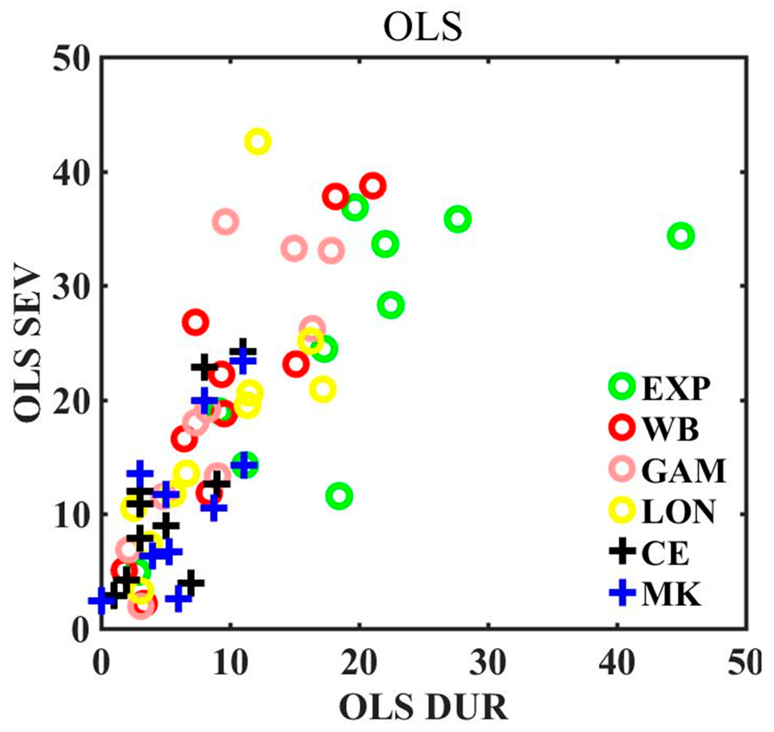
The X-axis and Y-axis in Figure 3 present the sum of squared errors (SSEs) in the OLS criterion for drought duration and drought severity for 10 stations across China, respectively. A smaller SSE value represents a better performance [76]. As shown in the figure, empirical distributions based on the two MMEs show robust results for both drought duration and drought severity over the 10 stations. This proves the superiority of utilizing the MMEs in frequency analysis for extreme climate events and the rationality of employing an empirical distribution.
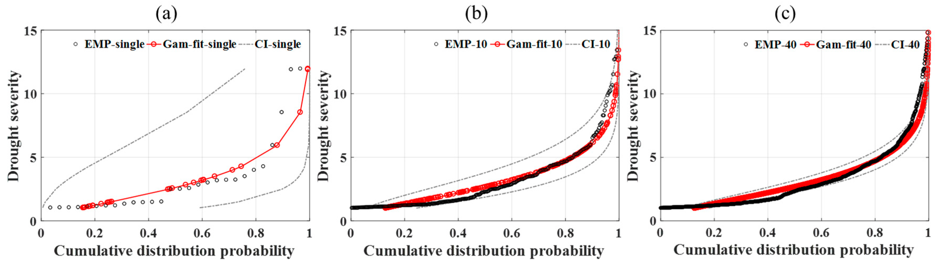
To further examine the superiority of empirical distributions based on large sample sizes provided by the MMEs, cumulative distributions of the drought severity using the different number of simulations (one-member, 10-member and 40-member simulations) of CESM1 for one station in China were analyzed in Figure 4. Here, the gamma distribution was used to serve as a comparison. As represented by the confidence intervals (CI) in Figure 4, the fitting uncertainty, which is mainly derived from parameter estimation, will significantly decline with increasing sample sizes. This shows that frequency analysis, which is based on a large sample size, will be more reliable. However, the corresponding fitting error will also increase with increase in sample sizes, especially for the tail, as indicated by pronounced disparities between the empirical distributions and the gamma distributions. This increasing fitting error will thus partially weaken the superiority of large sample sizes. On the other hand, empirical distributions characterize authentic features of a sample when the sample size is large enough. Therefore, it is reliable to employ empirical distributions combined with MMEs in frequency analysis.
3.5. Data Analysis
In order to quantify the effects of bias correction and future changes in drought conditions, the relative errors (RE) between MMEs and observed precipitation in the reference period—Equation (10)—and relative changes (RC) of drought variables between future and reference periods—Equation (11)—are calculated:
where RE represents the relative error, Vsim is the statistic (e.g., mean and SD) in MMEs precipitation and Vobs is the corresponding statistic in observed precipitation. As for RC, Vfut stands for the future drought variables (e.g., drought frequency, maximum drought duration and severity) and Vref stands for the corresponding variables in the reference period. Additionally, the statistical significance of the changes in drought frequency, drought duration, and drought severity in future periods relative to the reference period is tested by using the “Welch’s t test” [77,78]. When using the “Welch’s t test”, all values corresponding to drought frequency, drought duration, or drought severity from all members within the same period are pooled together to construct a sample. All stations with a significant climate change signal at the p = 0.05 significance level will be highlighted in figures.
4. Results
4.1. Validation of Downscaling Methods
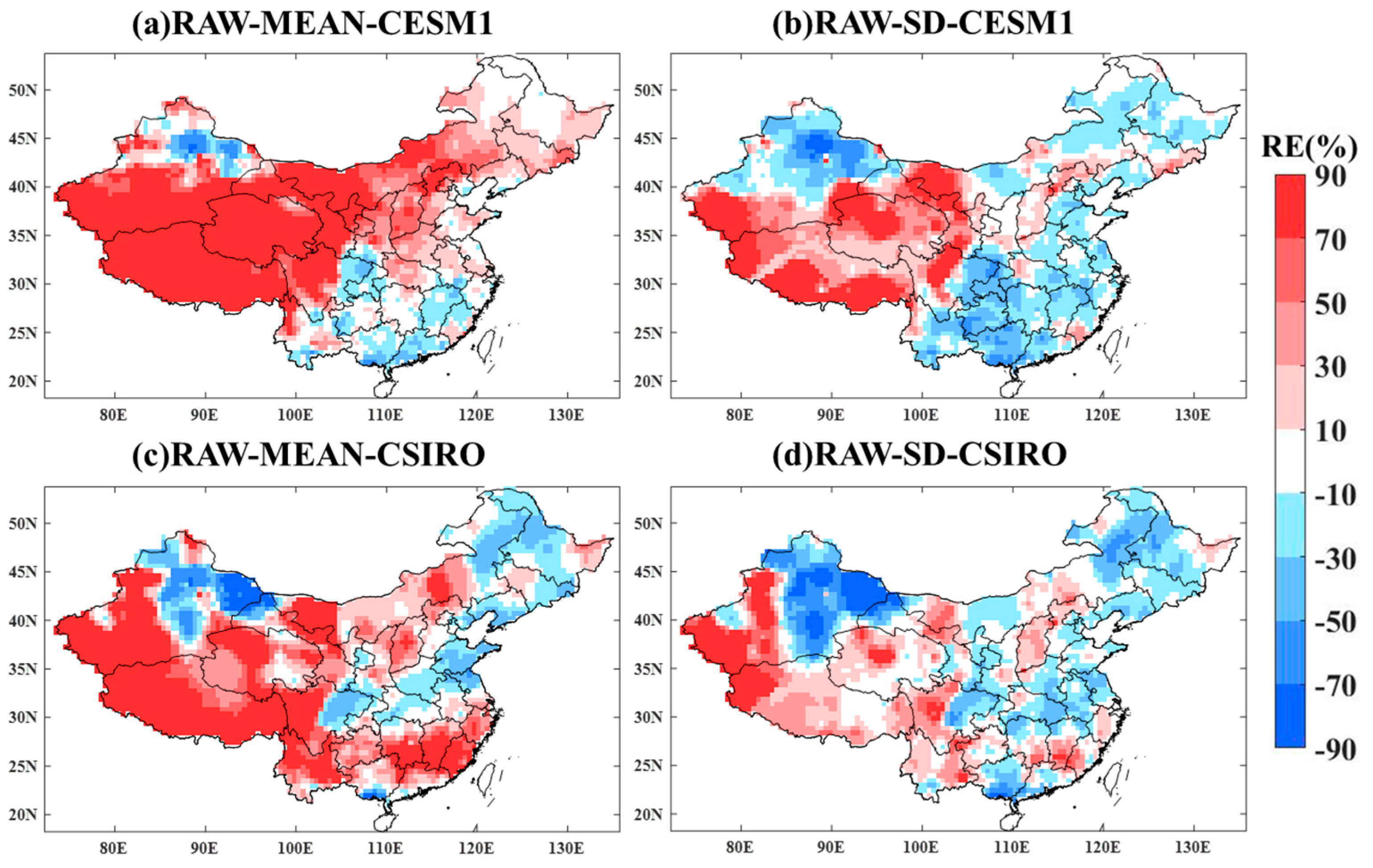
Figure 2 presents the relative errors of the mean and standard deviation for precipitation in July simulated by two climate model large ensembles without bias correction for the reference period. The relative error was calculated based on ensemble mean, rather than each individual member. Since similar correction performances are observed for all months, only results from July are presented in Figure 2 for illustration. Generally, both MMEs without post-processing are considerably biased in simulating mean July precipitation in China, with the relative errors ranging from −10% to 50% over most areas. Both ensembles overestimate mean precipitation in the Qinghai-Tibetan plateau. The CESM1 also overestimates mean precipitation in northern China and the CSIRO overestimates the mean values in southern China. On the other hand, the CESM1 underestimates mean precipitation for southeastern China, whereas the CSIRO underestimates the mean values for central and northeastern China.
The relative errors of the standard deviation (SD) range from −10% to 30% for CESM1- and CSIRO-simulated July precipitation over most stations. Both climate model ensembles (especially the CESM1) overestimate the SD in the arid Qinghai-Tibetan plateau. In addition, for all other regions, the SD of precipitation is generally underestimated by both ensembles, with the exception of some southwestern regions, where the SD of July precipitation is overestimated by the CSIRO.
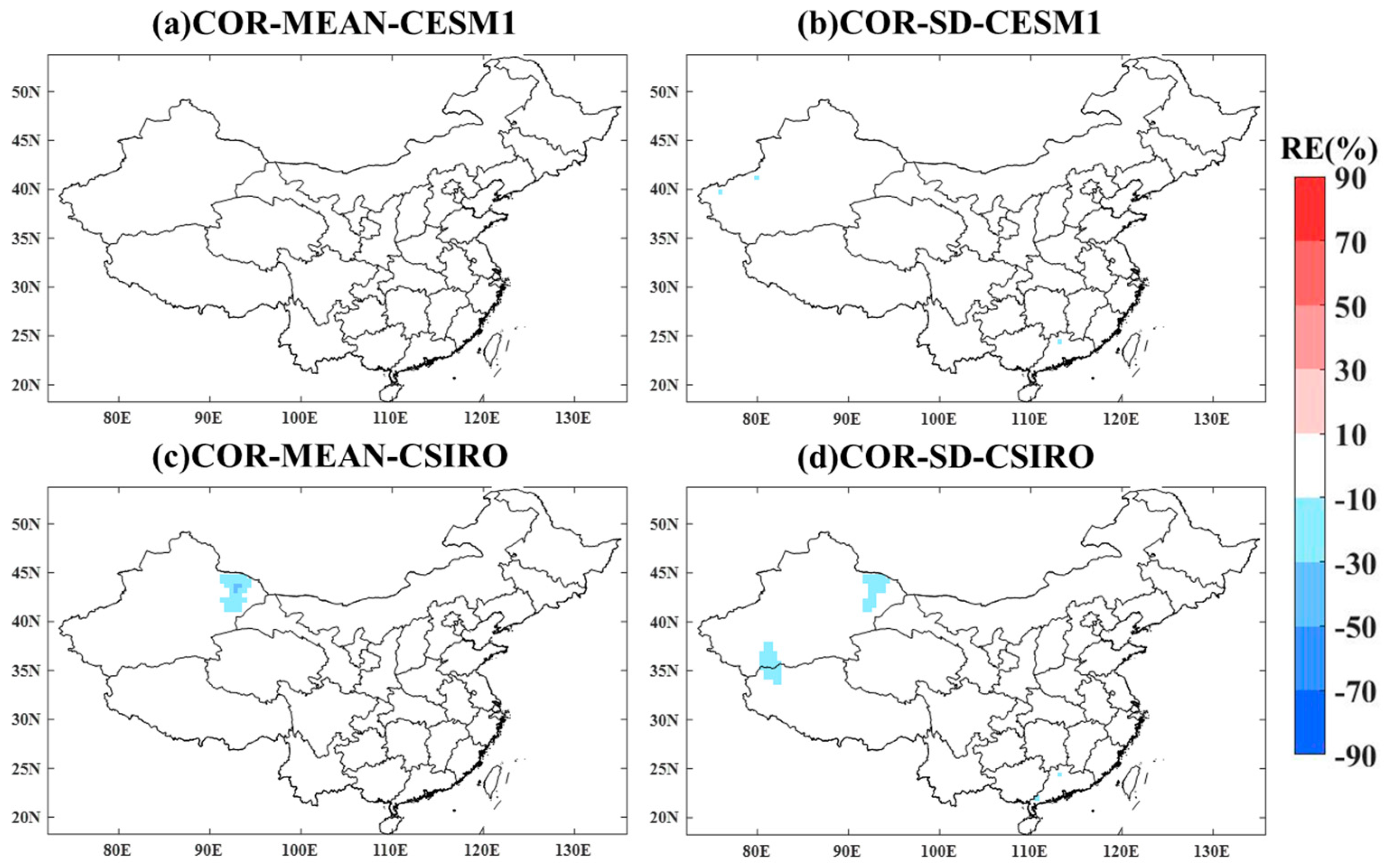
For the bias-corrected precipitation, both the mean and the SD are almost identical to that of observations all over China, as indicated by the white background in Figure 5. This proves the reasonable performance of the bias correction method for multi-member climate ensembles.
4.2. Future Drought Frequencies
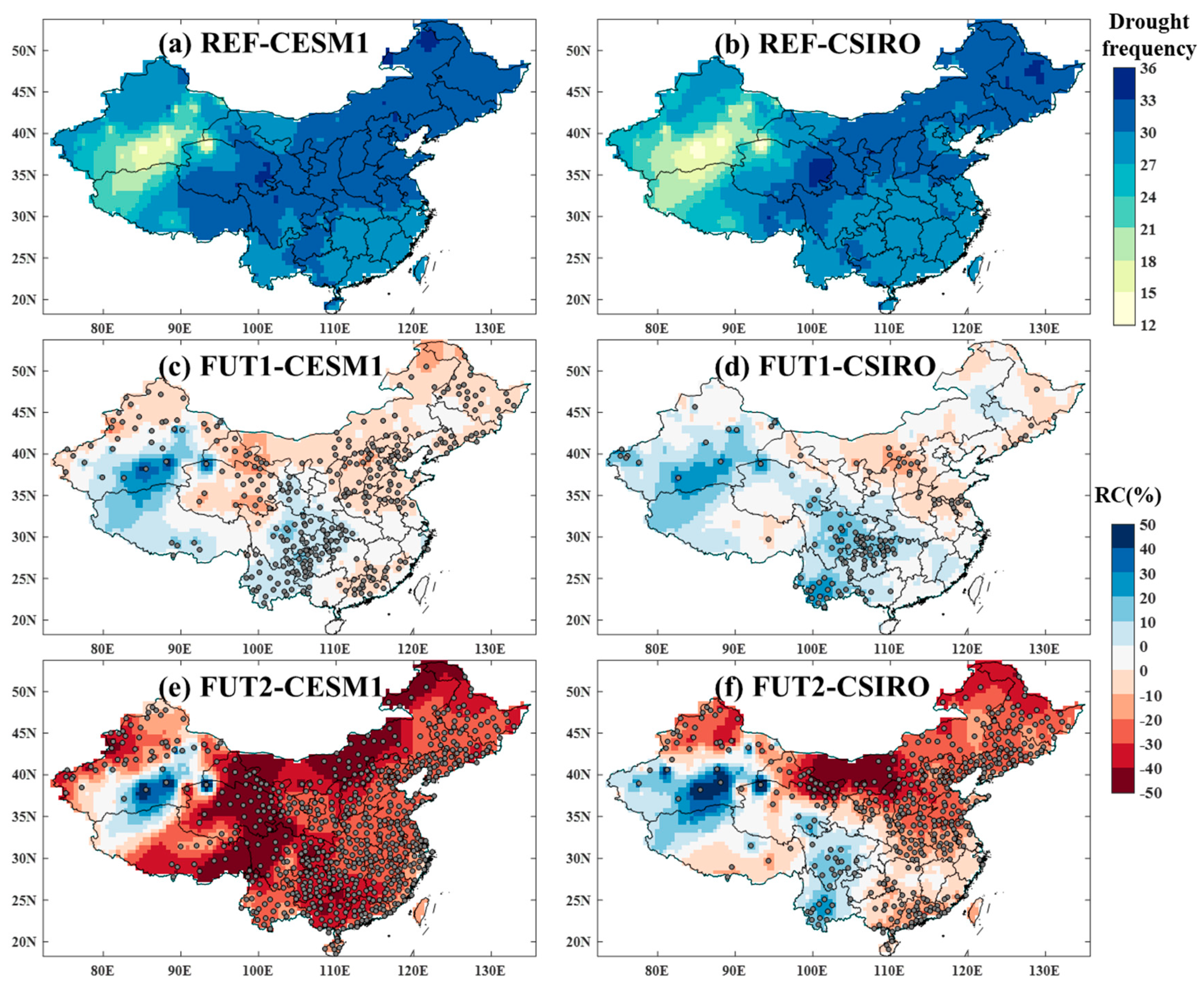
Figure 6 presents frequencies of droughts (defined by the threshold value of −1 for SPI) simulated by two MMEs for the reference period and their relative changes for the near and far future periods. In the reference period, the drought frequency ranges between 12 and 34 times for CESM1 and between 12 and 35 times for CSIRO, across all stations in China. Even though the range of drought frequency is similar between two climate models, the uncertainty related to climate models cannot be neglected, as indicated by the higher drought frequency simulated by CESM1 for most regions in China. The low drought frequency in the reference period tends to appear in northwestern China, whereas the high drought frequency is mainly located in northeastern and central China. Additionally, moderate drought frequencies can be seen in southern China.
In the near future, changes in drought frequencies vary among different regions. A half of stations show statistically significant changes at the p = 0.05 level, when using CESM1. The percentile of stations is 20% when using CSIRO. Generally, the frequency is projected to increase in western China, with relative changes ranging between 10 and 30%. On the other hand, a slight decrease of drought frequency can be seen in northern and northeastern China, approximately ranging between −10 and −20% for the CESM1 and CSIRO. The climate model uncertainty can also be inspected by the two climate model ensembles. For example, CESM1 projects a decrease in drought frequency in northern China, while CSIRO projects a much weaker decrease or even an opposite sign in some northern regions.
Changes of drought frequencies in the far future can exceed that of the near future, in spite of considerable inconsistency between the two multi-member ensembles (Figure 6e,f). The ratio of stations that show significant changes can reach up to 99% for CESM1 (and 64% for CSIRO). Compared with the near future period, projected changes in the end of century are less certain, especially in southwestern China where the CESM1 projects a decline in drought frequency while the CSIRO projects an increasing change. Parts of northwestern China present rising frequency ranging between 20 and 50% projected by CSIRO, in line with the case of CESM1. On the other hand, negative frequency changes are projected by CESM1 and CSIRO in northeastern China. Considerably decreasing frequency of droughts is projected to appear in northern China with relative changes approaching about −50%. In contrast, southeastern China will experience a slight decrease in the frequency of droughts with relative changes varying from −10 to −20%.
4.3. Future Drought Hazards
The future drought hazards represented by 30- and 50-year return periods of drought duration and drought severity are analyzed based on the empirical distribution.
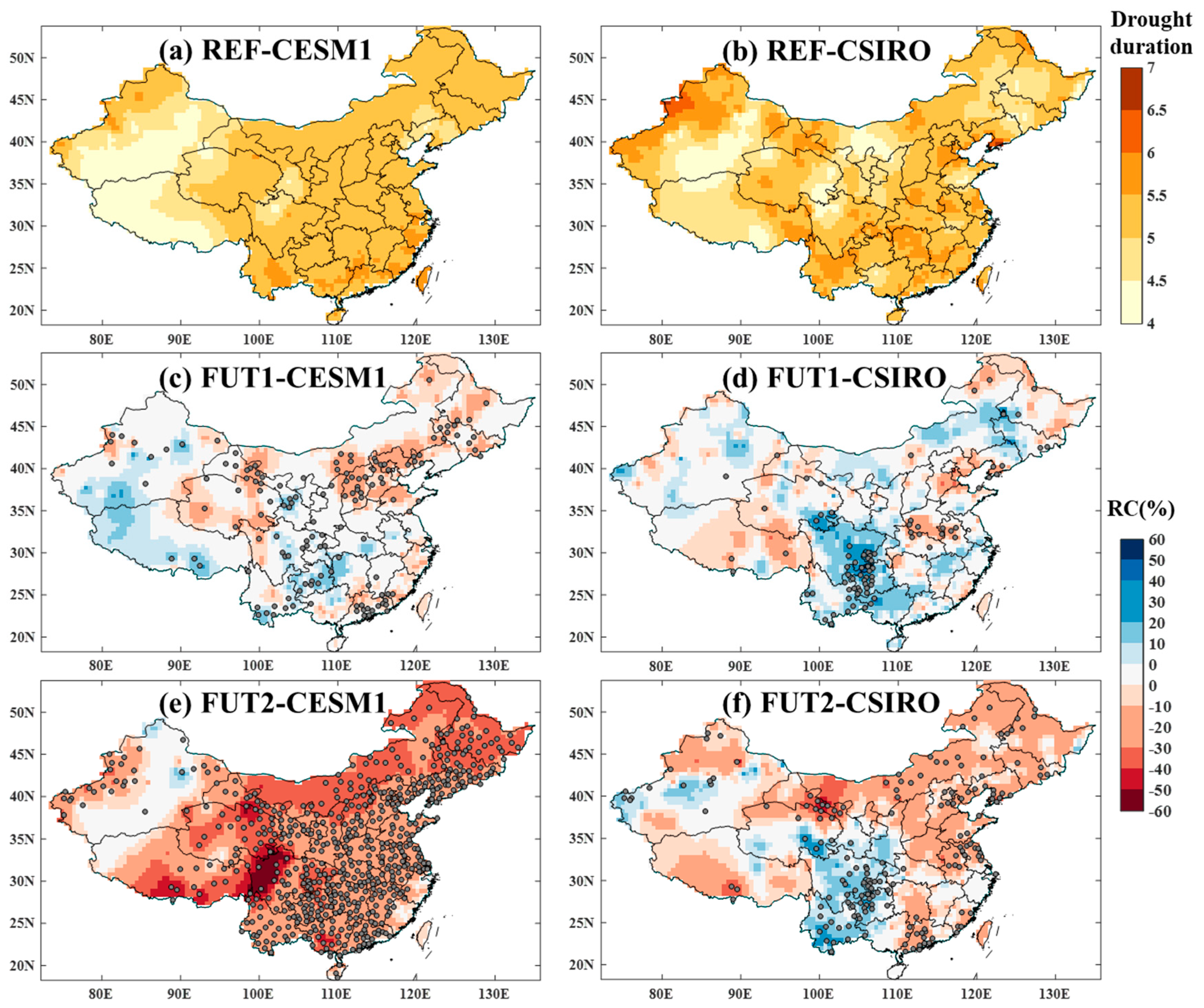
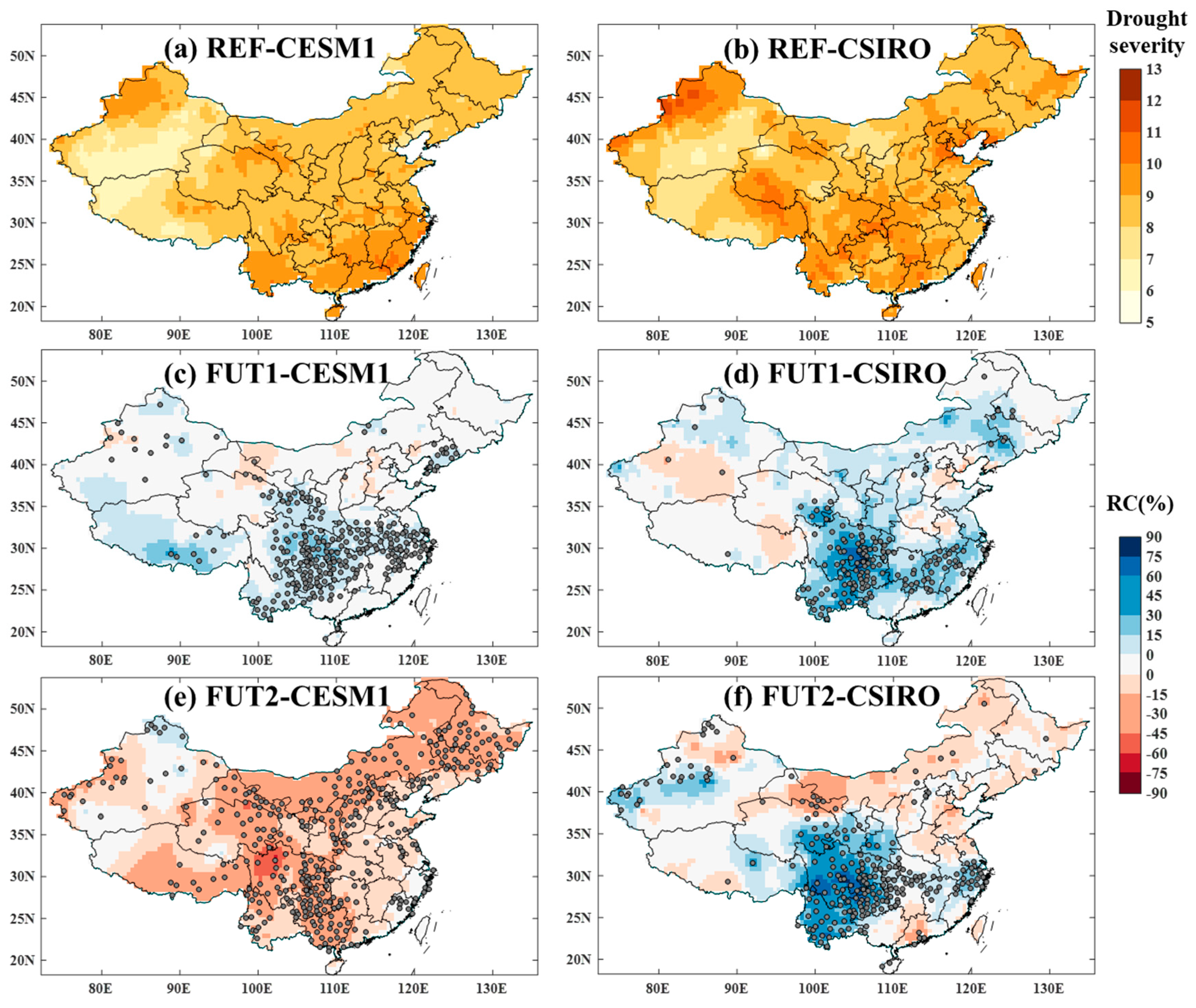
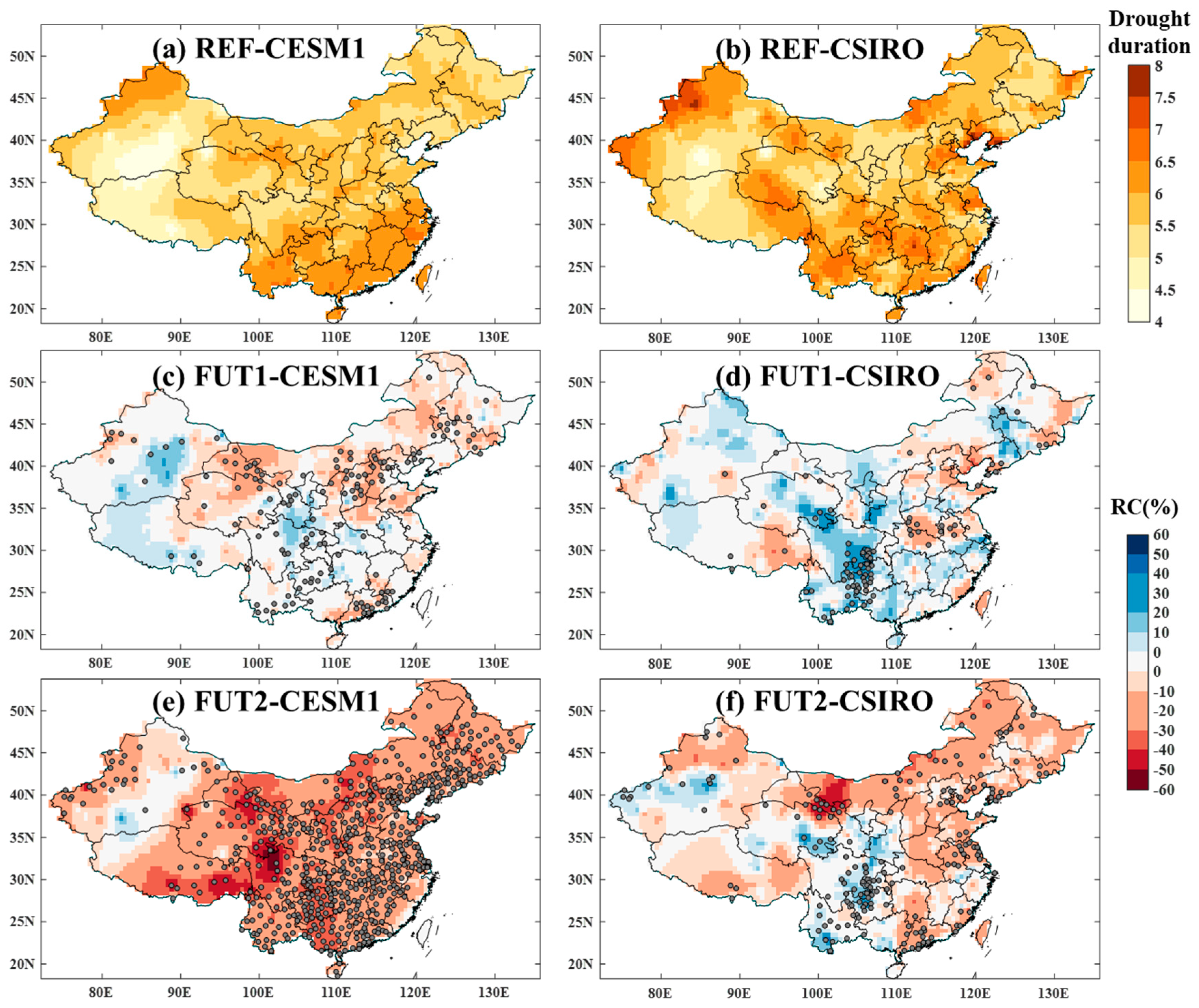
Figure 7 and Figure 8 present the 30-year return periods of drought duration and drought severity in China for the reference period and their relative changes for two future periods. In the reference period, there exists distinctive spatial variability for the 30-year return period in terms of drought duration and drought severity across China. The 30-year return period of drought duration simulated by CESM1 ranges between 4 and 7 months and the 30-year return period of drought severity ranges between 5 and 13. A larger spatial variability is projected by CSIRO with the 30-year return period of drought duration ranging from 4 to 11 months and drought severity ranging from 7 to 21. Additionally, the spatial patterns of the 50-year return levels (Figure 9 and Figure 10) are quite similar with that of the 30-year return levels for both drought duration and drought severity.
In the near future, deteriorating drought hazards represented by 30-year return periods of drought duration and drought severity can be observed in most regions over China. When using CESM1, more stations show statistically significant changes for both drought duration and drought severity than using CSIRO. Generally, the relative changes of 30-year return period of drought severity are projected to be more remarkable than that of 30-year return period of drought duration, with more pronounced changes projected by CSIRO than that by CESM1. Specifically, CSIRO projects a relative change in 30-year return period of drought duration ranging between −33% and 60% across China and a relative change in 30-year return period of drought severity ranging between −34% and 83%. The values range between −27% and 45% (drought severity) and between −33% and 25% (drought duration) for CESM1. For relative changes in 50-year return levels, their spatial patterns are similar to that in 30-year return levels for both drought duration and drought severity. However, CSIRO projects a slightly more prominent spatial variability than CESM1 for both drought duration and drought severity.
For the far future period, the amplitudes of changes in drought hazards represented by 30- and 50-return periods of drought duration and drought severity are further extended. The number of stations that show statistically significant changes for both drought duration and drought severity will also increase during this period for both models. In addition, a lesser agreement can be observed between the two climate models. Generally, in contrast to the near future period, drought hazards are projected to be alleviated for the far future period with more significant and widespread negative changes across China. In specific, the negative change is more pronounced for the 30-year return period of drought severity compared with that for the 30-year return period of drought duration. In addition, CESM1 projects more negative changes in both 30-year return period of drought duration and drought severity than CSIRO. With an exception of a few stations in the northwestern regions, the drought hazards projected by CESM1 will be relieved across China with the lowest value up to −60% for the 30-year return period of drought duration and −67% for the 30-year return period of drought severity. However, a larger spatial variability is projected by CSIRO. Similar magnitudes and spatial patterns of drought duration and drought severity are observed for 50-year return periods.
5. Discussion
Internal climate variability (ICV) is one of the major components contributing to climate change, especially for the historical period with less external forcing from greenhouse gas emissions [79]. However, it is usually not considered in climate change impact studies, as long time series used to represent the ICV are usually not available. The development of MMEs provides an opportunity to consider ICV in climate change impact studies. The MME is achieved by running a climate model several times with the same climate forcing, but different initial conditions. Remarkably different climate scenarios may be predicted in a MME, even though a very minor change had been made in the initial conditions of a climate model. Thus, each member contains information of intrinsic variability in the climate system and its responses under human-induced climate change. Any member can be considered as a possible realization of real climate if model biases are not considered. Thus, the inter-member difference can represent the ICV in a climate system, and all members can be assembled to investigate the role of ICV in climate change impacts. Until now, MMEs of several climate models have been developed and widely used in climate change studies [41,42]. These MMEs perform reasonably well with respect to reproducing the long-term observed ICV of mean precipitation and temperature, especially at multi-decadal scales [54].
It is well known that the climate model itself is one of the largest uncertainty contributors to climate change impacts [79]. Due to data availability, only two climate models with large ensemble members were used in this study. Other climate models in the Coupled Model Inter-comparison Project Phase 5 (CMIP5) database usually have fewer ensemble members, which could be inadequate to represent the ICV. Even though it would be better to include more models, the two models applied here reflect the model uncertainty to a certain extent, especially for the far future period. For example, the disparities in spatial distributions of changes in drought frequencies, 30- and 50-year return periods of drought duration, and drought severity between CESM1 and CSIRO all become more remarkable in the far future period than in the near future. Besides, the uncertainty is pronounced in southwestern China where two models suggest different directions of drought changes for the far future period. In addition, though the CSIRO contains fewer runs than the CESM1, it often presents more significant changes, as indicated by larger amplitudes in drought frequencies, 30- and 50-year return periods of drought duration, and drought severity for the two future periods. Overall, different model structures combined with different initial conditions may lead to divergent inter-member variability and subsequently result in divergent spatial patterns and corresponding absolute values.
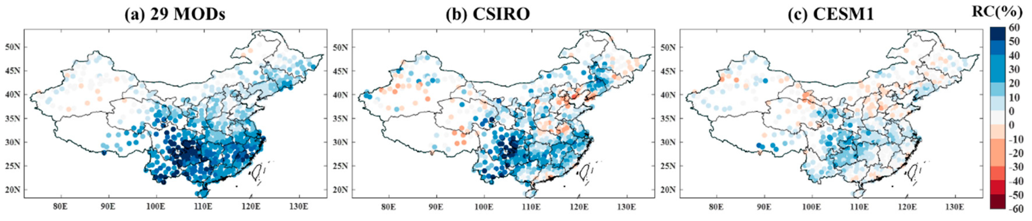
To better reveal the role of ICV in future drought projections, the results of climate change impacts with and without the consideration of ICV are demonstrated as follows by comparing the multi-member-ensemble (CSIRO or CESM1) with the multi-model-ensemble (single simulations from 29 climate models) in estimating the relative changes of 30-year return period of drought severity between the near future and the reference period in China (Figure 11). When using the multi-member-ensemble, an empirical distribution was fitted based on samples of all members to calculate return periods of drought severity. When using the multi-model-ensemble, the average of 29 climate models with a single simulation was used. Specifically, a single simulation was used to calculate the 30-year return period of drought severity based on the gamma distribution. The mean value was then calculated over all 29 climate models. As shown in Figure 11, without consideration of ICV, more stations in China present deteriorating drought hazards, as indicated by the increase in the 30-year return period of drought severity. Even though it is unable to determine which method is more reliable in estimating the climate change impacts on drought, the use of multi-member ensemble specifically considers the effects of ICV, which is an irreducible uncertainty source for impact studies.
Moreover, the signal to uncertainty ratio (SNR, [80]) of changes in drought frequency for the near future period relative to the reference period was also calculated (Figure 12). The signal is defined as the mean of future changes in drought frequency over all 29 climate models. The uncertainty related to the choice of a climate model was compared to that related to the ICV in estimating the changes of drought frequency. Specifically, the uncertainty related to climate models was defined as the standard deviation of changes in climate change signals projected by 29 climate model simulations. The uncertainty related to ICV was defined as the inter-member variability (standard deviation) of the multi-member ensemble (CSIRO or CESM1). As shown in Figure 12, the uncertainty related to ICV is comparable to that related to climate models. In addition, the ICV plays a significant role in drought impact studies, especially for southern China, where the SNR is smaller than 1. This further indicates the necessity of taking into account the ICV in climate change impact studies.
Overall, the results presented in Figure 11 and Figure 12 indicate that the ICV contributes large uncertainty in drought projections and plays a significant role in climate change impacts on droughts. Thus, the impacts of ICV should be specifically considered in drought projections. Since the observed time series is usually not long enough to manifest the ICV, especially at the multi-decadal scale, the use of multi-member ensemble is an alternative solution. In fact, if multi-member ensembles are available for all climate models, it is ideal to use all of them to adequately represent the overall uncertainty from climate models and ICV [81,82]. However, it is computationally too expensive to run all climate models with multiple members. Since previous studies [54] have shown that the multi-member ensemble of a climate model can reasonably represent the observed ICV, especially at the multi-decadal scale, when the ensemble member is larger than 5, a compromise solution may combine multi-model ensembles with multi-member ensemble for impact studies. This may be achieved by adding the ICV estimated using a single multi-member ensemble on the top of the climate change signal estimated using multi-model ensembles. This can be an avenue for future studies.
As mentioned in the Introduction, droughts have several categories; this study only considered meteorological drought because other types of droughts are basically derived from meteorological drought and especially abnormal precipitation conditions. In fact, the assessment of other types of droughts follows a similar framework. The differences mainly lie in the selection of hydro-meteorological variables and criteria. In order to describe drought conditions more systematically, more drought indices from various hydro-meteorological variables should be conducted in future studies.
Moreover, drought duration and drought severity may be dependent on each other [26], but the univariate return periods/levels calculated in this study ignored this dependence. However, this dependence can be induced by using joint distributions for drought duration and severity, such as copula functions or conditional distributions. This will also be an avenue for future studies.
6. Conclusions
In this paper, two MMEs are employed to investigate the joint impacts of ICV and anthropogenic climate change on future meteorological drought conditions. Based on the large sample size provided by MMEs, the empirical distributions are able to be used in frequency analysis to depict drought hazards. The following conclusions can be drawn.
- (1)
- Precipitation predictions simulated by CESM1 and CSIRO ensembles have considerable biases, while these biases can be effectively reduced by the bias correction method.
- (2)
- Based on bias-corrected CESM1 and CSIRO ensembles, northwestern China experiences mild drought conditions in the reference period, as indicated by low drought frequencies and hazards. Remarkably frequent droughts with relatively short drought duration and small drought severity are found in northeastern China. Southern China is subject to moderate drought frequencies but with long drought duration and large drought severity.
- (3)
- In the middle of the 21st century, CESM1 and CSIRO ensembles project decreases in the drought frequency and drought duration in northern and northeastern China, and increases in drought severity, resulting in shorter but heavier droughts. In contrast, drought conditions will significantly deteriorate in southwestern China, while drought frequencies will go up and the 30- and 50-year drought duration and severity will increase.
- (4)
- At the end of the 21st century, drought frequencies and drought hazards are projected to decrease in northern and, especially, northeastern China for both climate models. However, a large uncertainty related to climate models is observed when simulating drought conditions. For example, drought conditions will continue to deteriorate in southwestern China under the CSIRO, while they will greatly alleviate under the CESM1.
Author Contributions
Conceptualization, L.G. and J.C.; methodology, L.G.; software, L.G.; validation, J.C., C.-Y.X. and H.-M.W.; formal analysis, L.G.; investigation, L.G.; resources, L.G.; data curation, L.G.; writing—original draft preparation, L.G.; writing—review and editing, J.C., C.-Y.X., H.-M.W., L.Z.; visualization, L.Z.; supervision, J.C.; project administration, L.Z.; funding acquisition, J.C.
Funding
This research was funded by the National Key Research and Development Program of China (No. 2017YFA0603704), the National Natural Science Foundation of China (No. 51779176) and the Thousand Youth Talents Plan from the Organization Department of the CCP Central Committee (Wuhan University, China).
Acknowledgments
The authors wish to thank the China Meteorological Data Sharing Service System for providing gauged precipitation for China, the contribution of the World Climate Research Program Working Group on Coupled Modelling for making available their climate model outputs (CSIRO MK3.6), and the CEMS1 (CAM) large ensemble community project for providing the large ensemble of CESM1 data.
Conflicts of Interest
The authors declare that they have no conflict of interest.
References
- Feyen, L.; Dankers, R. Impact of global warming on streamflow drought in Europe. J. Geophys. Res. 2009, 114. [Google Scholar] [CrossRef] [Green Version]
- Zeng, N. Drought in the Sahel. Science 2003, 302, 999–1000. [Google Scholar] [CrossRef] [PubMed]
- Rodríguez-Fonseca, B.; Mohino, E.; Mechoso, C.R.; Caminade, C.; Biasutti, M.; Gaetani, M.; Garcia-Serrano, J.; Vizy, E.K.; Cook, K.; Xue, Y.; et al. Variability and Predictability of West African Droughts: A Review on the Role of Sea Surface Temperature Anomalies. J. Clim. 2015, 28, 4034–4060. [Google Scholar] [CrossRef] [Green Version]
- Qiu, J. China drought highlights future climate threats. Nature 2010, 465, 142–143. [Google Scholar] [CrossRef] [PubMed] [Green Version]
- Li, Y.; Chen, C.; Sun, C. Drought severity and change in Xinjiang, China, over 1961–2013. Hydrol. Res. 2017, 48, 1343–1362. [Google Scholar] [CrossRef]
- Wong, G.; Lambert, M.F.; Leonard, M.; Metcalfe, A.V. Drought Analysis Using Trivariate Copulas Conditional on Climatic States. J. Hydrol. Eng. 2010, 15, 129–141. [Google Scholar] [CrossRef]
- Ummenhofer, C.C.; England, M.H.; McIntosh, P.C.; Meyers, G.A.; Pook, M.J.; Risbey, J.S.; Gupta, A.S.; Taschetto, A.S. What causes southeast Australia’s worst droughts? Geophys. Res. Lett. 2009, 36. [Google Scholar] [CrossRef]
- Kiem, A.S.; Johnson, F.; Westra, S.; van Dijk, A.; Evans, J.P.; O’Donnell, A.; Rouillard, A.; Barr, C.; Tyler, J.; Thyer, M.; et al. Natural hazards in Australia: Droughts. Clim. Chang. 2016, 139, 37–54. [Google Scholar] [CrossRef]
- Le Comte, D. Weather Highlights: Around the World. Weatherwise 2010, 51, 26–31. [Google Scholar] [CrossRef]
- Changnon, S.A.; Pielke, R.A.; Changnon, D.; Sylves, R.T.; Pulwarty, R. Human Factors Explain the Increased Losses from Weather and Climate Extremes*. Bull. Am. Meteorol. Soc. 2000, 81, 437–442. [Google Scholar] [CrossRef] [Green Version]
- Hopkins, B. The effects of the 1976 drought on chalk grassland in Sussex, England. Biol. Conserv. 1978, 14, 1–12. [Google Scholar] [CrossRef]
- Mishra, A.K.; Singh, V.P. A review of drought concepts. J. Hydrol. 2010, 391, 202–216. [Google Scholar] [CrossRef]
- Esfahanian, E.; Nejadhashemi, A.P.; Abouali, M.; Adhikari, U.; Zhang, Z.; Daneshvar, F.; Herman, M.R. Development and evaluation of a comprehensive drought index. J. Environ. Manag. 2017, 185, 31–43. [Google Scholar] [CrossRef] [PubMed]
- Ayantobo, O.O.; Li, Y.; Song, S.; Yao, N. Spatial comparability of drought characteristics and related return periods in mainland China over 1961–2013. J. Hydrol. 2017, 550, 549–567. [Google Scholar] [CrossRef]
- Qin, Y.; Yang, D.; Lei, H.; Xu, K.; Xu, X. Comparative analysis of drought based on precipitation and soil moisture indices in Haihe basin of North China during the period of 1960–2010. J. Hydrol. 2015, 526, 55–67. [Google Scholar] [CrossRef]
- Liu, Z.; Wang, Y.; Shao, M.; Jia, X.; Li, X. Spatiotemporal analysis of multiscalar drought characteristics across the Loess Plateau of China. J. Hydrol. 2016, 534, 281–299. [Google Scholar] [CrossRef] [Green Version]
- Zhu, Y.; Chang, J.; Huang, S.; Huang, Q. Characteristics of integrated droughts based on a nonparametric standardized drought index in the Yellow River Basin, China. Hydrol. Res. 2015, 47, 454–467. [Google Scholar] [CrossRef]
- Rivera, J.A.; Araneo, D.C.; Penalba, O.C.; Villalba, R. Regional aspects of streamflow droughts in the Andean rivers of Patagonia, Argentina. Links with large-scale climatic oscillations. Hydrol. Res. 2018, 49, 134–149. [Google Scholar] [CrossRef]
- Ye, X.; Li, X.; Xu, C.-Y.; Zhang, Q. Similarity, difference and correlation of meteorological and hydrological drought indices in a humid climate region—The Poyang Lake catchment in China. Hydrol. Res. 2016, 47, 1211–1223. [Google Scholar] [CrossRef]
- Katz, R.W.; Parlange, M.B.; Naveau, P. Statistics of extremes in hydrology. Adv. Water Resour. 2002, 25, 1287–1304. [Google Scholar] [CrossRef] [Green Version]
- Zhu, B.; Xie, X.; Zhang, K. Water storage and vegetation changes in response to the 2009/10 drought over North China. Hydrol. Res. 2018, 49, 1618–1635. [Google Scholar] [CrossRef]
- Haro-Monteagudo, D.; Daccache, A.; Knox, J. Exploring the utility of drought indicators to assess climate risks to agricultural productivity in a humid climate. Hydrol. Res. 2018, 49, 539–551. [Google Scholar] [CrossRef]
- Chitsaz, N.; Hosseini-Moghari, S.-M. Introduction of new datasets of drought indices based on multivariate methods in semi-arid regions. Hydrol. Res. 2018, 49, 266–280. [Google Scholar] [CrossRef]
- Safavi, H.R.; Raghibi, V.; Mazdiyasni, O.; Mortazavi-Naeini, M. A new hybrid drought-monitoring framework based on nonparametric standardized indicators. Hydrol. Res. 2018, 49, 222–236. [Google Scholar] [CrossRef]
- Xu, K.; Yang, D.; Yang, H.; Li, Z.; Qin, Y.; Shen, Y. Spatio-temporal variation of drought in China during 1961–2012: A climatic perspective. J. Hydrol. 2015, 526, 253–264. [Google Scholar] [CrossRef]
- Chang, J.; Li, Y.; Wang, Y.; Yuan, M. Copula-based drought risk assessment combined with an integrated index in the Wei River Basin, China. J. Hydrol. 2016, 540, 824–834. [Google Scholar] [CrossRef]
- Mondal, A.; Mujumdar, P.P. Return levels of hydrologic droughts under climate change. Adv. Water Resour. 2015, 75, 67–79. [Google Scholar] [CrossRef]
- Burke, E.J.; Perry, R.H.J.; Brown, S.J. An extreme value analysis of UK drought and projections of change in the future. J. Hydrol. 2010, 388, 131–143. [Google Scholar] [CrossRef]
- Sheffield, J.; Wood, E.F. Projected changes in drought occurrence under future global warming from multi-model, multi-scenario, IPCC AR4 simulations. Clim. Dyn. 2007, 31, 79–105. [Google Scholar] [CrossRef]
- Dai, A. Increasing drought under global warming in observations and models. Nat. Clim. Chang. 2012, 3, 52–58. [Google Scholar] [CrossRef]
- Naumann, G.; Spinoni, J.; Vogt, J.V.; Barbosa, P. Assessment of drought damages and their uncertainties in Europe. Environ. Res. Lett. 2015, 10, 124013. [Google Scholar] [CrossRef] [Green Version]
- Martel, J.-L.; Mailhot, A.; Brissette, F.; Caya, D. Role of Natural Climate Variability in the Detection of Anthropogenic Climate Change Signal for Mean and Extreme Precipitation at Local and Regional Scales. J. Clim. 2018, 31, 4241–4263. [Google Scholar] [CrossRef]
- Yin, J.; Gentine, P.; Zhou, S.; Sullivan, S.C.; Wang, R.; Zhang, Y.; Guo, S. Large increase in global storm runoff extremes driven by climate and anthropogenic changes. Nat. Commun. 2018, 9, 4389. [Google Scholar] [CrossRef] [PubMed]
- Yin, J.; Guo, S.; He, S.; Guo, J.; Hong, X.; Liu, Z. A copula-based analysis of projected climate changes to bivariate flood quantiles. J. Hydrol. 2018, 566, 23–42. [Google Scholar] [CrossRef]
- Stocker, T.F. Summary for policymakers. In Climate Change 2013: The Physical Science Basis; Working Group I Contribution to the Fifth Assessment Report of the Intergovernmental Panel on Climate Change; Cambridge University Press: Cambridge, UK, 2013. [Google Scholar]
- Fischer, E.M.; Knutti, R. Anthropogenic contribution to global occurrence of heavy-precipitation and high-temperature extremes. Nat. Clim. Chang. 2015, 5, 560–564. [Google Scholar] [CrossRef]
- Perkins, S.E.; Fischer, E.M. The usefulness of different realizations for the model evaluation of regional trends in heat waves. Geophys. Res. Lett. 2013, 40, 5793–5797. [Google Scholar] [CrossRef] [Green Version]
- Sheffield, J.; Wood, E.F.; Roderick, M.L. Little change in global drought over the past 60 years. Nature 2012, 491, 435–438. [Google Scholar] [CrossRef] [PubMed]
- Trenberth, K.E.; Dai, A.; van der Schrier, G.; Jones, P.D.; Barichivich, J.; Briffa, K.R.; Sheffield, J. Global warming and changes in drought. Nat. Clim. Chang. 2014, 4, 17–22. [Google Scholar] [CrossRef]
- Orlowsky, B.; Seneviratne, S.I. Elusive drought: Uncertainty in observed trends and short- and long-term CMIP5 projections. Hydrol. Earth Syst. Sci. 2013, 17, 1765–1781. [Google Scholar] [CrossRef]
- Kay, J.E.; Deser, C.; Phillips, A.; Mai, A.; Hannay, C.; Strand, G.; Arblaster, J.M.; Bates, S.C.; Danabasoglu, G.; Edwards, J.; et al. The Community Earth System Model (CESM) Large Ensemble Project: A Community Resource for Studying Climate Change in the Presence of Internal Climate Variability. Bull. Am. Meteorol. Soc. 2015, 96, 1333–1349. [Google Scholar] [CrossRef]
- Deser, C.; Phillips, A.; Bourdette, V.; Teng, H. Uncertainty in climate change projections: The role of internal variability. Clim. Dyn. 2010, 38, 527–546. [Google Scholar] [CrossRef]
- Van Genderen, J.L. Drought: Past problems and future scenarios. Int. J. Digit. Earth 2012, 5, 456–457. [Google Scholar] [CrossRef]
- Chen, J.; St-Denis, B.G.; Brissette, F.P.; Lucas-Picher, P. Using Natural Variability as a Baseline to Evaluate the Performance of Bias Correction Methods in Hydrological Climate Change Impact Studies. J. Hydrometeorol. 2016, 17, 2155–2174. [Google Scholar] [CrossRef]
- Deser, C.; Knutti, R.; Solomon, S.; Phillips, A.S. Communication of the role of natural variability in future North American climate. Nat. Clim. Chang. 2012, 2, 775–779. [Google Scholar] [CrossRef]
- Zhuan, M.-J.; Chen, J.; Shen, M.-X.; Xu, C.-Y.; Chen, H.; Xiong, L.-H. Timing of human-induced climate change emergence from internal climate variability for hydrological impact studies. Hydrol. Res. 2018, 49, 421–437. [Google Scholar] [CrossRef]
- Meehl, G.A.; Washington, W.M.; Arblaster, J.M.; Hu, A.; Teng, H.; Kay, J.E.; Gettelman, A.; Lawrence, D.M.; Sanderson, B.M.; Strand, W.G. Climate Change Projections in CESM1(CAM5) Compared to CCSM4. J. Clim. 2013, 26, 6287–6308. [Google Scholar] [CrossRef]
- Lawrence, D.M.; Oleson, K.W.; Flanner, M.G.; Thornton, P.E.; Swenson, S.C.; Lawrence, P.J.; Zeng, X.; Yang, Z.-L.; Levis, S.; Sakaguchi, K.; et al. Parameterization improvements and functional and structural advances in Version 4 of the Community Land Model. J. Adv. Model. Earth Syst. 2011, 3. [Google Scholar] [CrossRef]
- Dai, A.; Fyfe, J.C.; Xie, S.-P.; Dai, X. Decadal modulation of global surface temperature by internal climate variability. Nat. Clim. Chang. 2015, 5, 555–559. [Google Scholar] [CrossRef]
- Rotstayn, L.D.; Collier, M.A.; Dix, M.R.; Feng, Y.; Gordon, H.B.; O’Farrell, S.P.; Smith, I.N.; Syktus, J. Improved simulation of Australian climate and ENSO-related rainfall variability in a global climate model with an interactive aerosol treatment. Int. J. Clim. 2009, 30, 1067–1088. [Google Scholar] [CrossRef]
- Rotstayn, L.D.; Jeffrey, S.J.; Collier, M.A.; Dravitzki, S.M.; Hirst, A.C.; Syktus, J.I.; Wong, K.K. Aerosol- and greenhouse gas-induced changes in summer rainfall and circulation in the Australasian region: A study using single-forcing climate simulations. Atmos. Chem. Phys. 2012, 12, 6377–6404. [Google Scholar] [CrossRef]
- Rotstayn, L.D.; Collier, M.A.; Chrastansky, A.; Jeffrey, S.J.; Luo, J.J. Projected effects of declining aerosols in RCP4.5: Unmasking global warming? Atmos. Chem. Phys. 2013, 13, 10883–10905. [Google Scholar] [CrossRef]
- Knutti, R.; Sedláček, J. Robustness and uncertainties in the new CMIP5 climate model projections. Nat. Clim. Chang. 2012, 3, 369–373. [Google Scholar] [CrossRef]
- Chen, J.; Brissette, F.P. Reliability of climate model multi-member ensembles in estimating internal precipitation and temperature variability at the multi-decadal scale. Int. J. Climatol. 2018. [Google Scholar] [CrossRef]
- Kling, H.; Fuchs, M.; Paulin, M. Runoff conditions in the upper Danube basin under an ensemble of climate change scenarios. J. Hydrol. 2012, 424–425, 264–277. [Google Scholar] [CrossRef]
- Fischer, E.M.; Schär, C. Consistent geographical patterns of changes in high-impact European heatwaves. Nat. Geosci. 2010, 3, 398–403. [Google Scholar] [CrossRef]
- Araujo, M.B.; Cabeza, M.; Thuiller, W.; Hannah, L.; Williams, P.H. Would climate change drive species out of reserves? An assessment of existing reserve-selection methods. Glob. Chang. Biol. 2004, 10, 1618–1626. [Google Scholar] [CrossRef]
- Immerzeel, W.W.; Pellicciotti, F.; Bierkens, M.F.P. Rising river flows throughout the twenty-first century in two Himalayan glacierized watersheds. Nat. Geosci. 2013, 6, 742–745. [Google Scholar] [CrossRef]
- Riahi, K.; Rao, S.; Krey, V.; Cho, C.; Chirkov, V.; Fischer, G.; Kindermann, G.; Nakicenovic, N.; Rafaj, P. RCP 8.5—A scenario of comparatively high greenhouse gas emissions. Clim. Chang. 2011, 109, 33–57. [Google Scholar] [CrossRef] [Green Version]
- Park, C.-K.; Byun, H.-R.; Deo, R.; Lee, B.-R. Drought prediction till 2100 under RCP 8.5 climate change scenarios for Korea. J. Hydrol. 2015, 526, 221–230. [Google Scholar] [CrossRef]
- Li, Y.; Huang, H.; Ju, H.; Lin, E.; Xiong, W.; Han, X.; Wang, H.; Peng, Z.; Wang, Y.; Xu, J.; et al. Assessing vulnerability and adaptive capacity to potential drought for winter-wheat under the RCP 8.5 scenario in the Huang-Huai-Hai Plain. Agric. Ecosyst. Environ. 2015, 209, 125–131. [Google Scholar] [CrossRef]
- Waseem, M.; Ajmal, M.; Kim, U.; Kim, T.-W. Development and evaluation of an extended inverse distance weighting method for streamflow estimation at an ungauged site. Hydrol. Res. 2016, 47, 333–343. [Google Scholar] [CrossRef]
- Schmidli, J.; Frei, C.; Vidale, P.L. Downscaling from GCM precipitation: A benchmark for dynamical and statistical downscaling methods. Int. J. Climatol. 2006, 26, 679–689. [Google Scholar] [CrossRef]
- Mpelasoka, F.S.; Chiew, F.H.S. Influence of rainfall scenario construction methods on runoff projections. J. Hydrometeorol. 2009, 10, 1168–1183. [Google Scholar] [CrossRef]
- Chen, J.; Brissette, F.P.; Leconte, R. Uncertainty of downscaling method in quantifying the impact of climate change on hydrology. J. Hydrol. 2011, 401, 190–202. [Google Scholar] [CrossRef]
- Jung, I.-W.; Moradkhani, H.; Chang, H. Uncertainty assessment of climate change impacts for hydrologically distinct river basins. J. Hydrol. 2012, 466–467, 73–87. [Google Scholar] [CrossRef]
- Chen, J.; Brissette, F.P.; Chaumont, D.; Braun, M. Performance and uncertainty evaluation of empirical downscaling methods in quantifying the climate change impacts on hydrology over two North American river basins. J. Hydrol. 2013, 479, 200–214. [Google Scholar] [CrossRef]
- Ahmadalipour, A.; Moradkhani, H.; Rana, A. Accounting for downscaling and model uncertainty in fine-resolution seasonal climate projections over the Columbia River Basin. Clim. Dyn. 2017, 50, 717–733. [Google Scholar] [CrossRef]
- Lee, J.H.; Kim, C.J. A multimodel assessment of the climate change effect on the drought severity-duration-frequency relationship. Hydrol. Process. 2013, 27, 2800–2813. [Google Scholar] [CrossRef]
- Zargar, A.; Sadiq, R.; Khan, F.I. Uncertainty-driven characterization of climate change effects on drought frequency using enhanced SPI. Water Resour. Manag. 2013, 28, 15–40. [Google Scholar] [CrossRef]
- Raziei, T.; Martins, D.S.; Bordi, I.; Santos, J.F.; Portela, M.M.; Pereira, L.S.; Sutera, A. SPI Modes of Drought Spatial and Temporal Variability in Portugal: Comparing Observations, PT02 and GPCC Gridded Datasets. Water Resour. Manag. 2014, 29, 487–504. [Google Scholar] [CrossRef]
- Yevjevich, V.M. An Objective Approach to Definitions and Investigations of Continental Hydrologic Droughts; Hydrology Papers No. 23; Colorado State University: Fort Collins, CO, USA, 1967. [Google Scholar]
- Shiau, J.-T.; Shen, H.W. Recurrence Analysis of Hydrologic Droughts of Differing Severity. J. Water Resour. Plan. Manag. 2001, 127, 30–40. [Google Scholar] [CrossRef]
- Shiau, J.-T.; Wang, H.-Y.; Tsai, C.-T. Bivariate Frequency Analysis of Floods Using Copulas1. J. Am. Water Resour. Assoc. 2006, 42, 1549–1564. [Google Scholar] [CrossRef]
- Ye, S.Z.; Zhan, D.J. Engineering Hydrology; China Water & Power Press: Beijing, China, 2000. (In Chinese) [Google Scholar]
- Singh, V.P.; Wang, S.X.; Zhang, L. Frequency analysis of nonidentically distributed hydrologic flood data. J. Hydrol. 2005, 307, 175–195. [Google Scholar] [CrossRef]
- Forzieri, G.; Feyen, L.; Rojas, R.; Flörke, M.; Wimmer, F.; Bianchi, A. Ensemble projections of future streamflow droughts in Europe. Hydrol. Earth Syst. Sci. 2014, 18, 85–108. [Google Scholar] [CrossRef] [Green Version]
- Welch, B.L. The Generalization of ‘Student’s’ Problem when Several Different Population Variances are Involved. Biometrika 1947, 34, 28–35. [Google Scholar] [CrossRef] [PubMed]
- Kumar, D.; Ganguly, A.R. Intercomparison of model response and internal variability across climate model ensembles. Clim. Dyn. 2017, 51, 207–219. [Google Scholar] [CrossRef]
- Hawkins, E.; Sutton, R. The Potential to Narrow Uncertainty in Regional Climate Predictions. Bull. Am. Meteorol. Soc. 2009, 90, 1095–1108. [Google Scholar] [CrossRef] [Green Version]
- Wang, H.-M.; Chen, J.; Cannon, A.J.; Xu, C.-Y.; Chen, H. Transferability of climate simulation uncertainty to hydrological impacts. Hydrol. Earth Syst. Sci. 2018, 22, 3739–3759. [Google Scholar] [CrossRef]
- Chen, J.; Brissette, F.P.; Lucas-Picher, P. Transferability of optimally-selected climate models in the quantification of climate change impacts on hydrology. Clim. Dyn. 2016, 47, 3359–3372. [Google Scholar] [CrossRef]
Figure 1.
Spatial distribution of the observed average (a); standard deviation (b); skewness (c); and kurtosis (d) annual precipitation in China for the period 1971–2000.
Figure 1.
Spatial distribution of the observed average (a); standard deviation (b); skewness (c); and kurtosis (d) annual precipitation in China for the period 1971–2000.

Figure 2.
The relative error (RE) of the mean (MEAN) and standard deviation (SD) for July precipitation for two climate model ensembles (CESM1; CSIRO) with raw (RAW) simulated data for the reference period (1971–2000). (a) The RE of the mean July precipitation for CESM1 with raw data; (b) The RE of the SD of July precipitation for CESM1 with raw data; (c) The RE of the mean July precipitation for CSIRO with raw data; (d) The RE of the SD of July precipitation for CSIRO with raw data.

Figure 3.
Ordinary least squares (OLSs) for both drought duration (DUR) and severity (SEV) for 10 stations across China. EXP, WB, GAM, LON represent the Exponential, Weibull, Gamma and Lognormal distributions, respectively. CE and MK represent empirical distributions based on the CESM1 and the CSIRO, respectively.

Figure 4.
Illustration of frequency analysis for drought severity under the empirical distribution (EMP, the dark circle) and the gamma distribution (Gam-fit, the red circle). The dashed grey line shows the 95% confidence intervals (CI) of the gamma distribution in parameter estimation. (a) The cumulative distributions based on one-member simulation of CESM1; (b)The cumulative distributions based on 10-member simulations of CESM1; (c)The cumulative distributions based on 40-member simulations of CESM1.

Figure 5.
The relative error (RE) of the mean (MEAN) and standard deviation (SD) for July precipitation for two climate model ensembles (CESM1; CSIRO) with (COR) bias correction for the reference period (1971–2000). (a) The RE of the mean July precipitation for CESM1 with corrected data; (b) The RE of the SD of July precipitation for CESM1 with corrected data; (c) The RE of the mean July precipitation for CSIRO with corrected data; (d) The RE of the SD of July precipitation for CSIRO with corrected data.

Figure 6.
Spatial pattern of drought frequency in the reference period (REF) and its relative changes (RC) for future periods (FUT1, FUT2) for two climate model ensembles. Stations that present statistically significant changes are marked with filled dots. (a) Drought frequency in REF for CESM1; (b) Drought frequency in REF for CSIRO; (c) The RC of drought frequency in FUT1 for CESM1; (d) The RC of drought frequency in FUT1 for CSIRO; (e) The RC of drought frequency in FUT2 for CESM1; (f) The RC of drought frequency in FUT2 for CSIRO.

Figure 7.
Spatial patterns of drought duration with a 30-year return period in the reference period (REF) and the relative changes (RC) in future periods (FUT1, FUT2) for two climate model ensembles. Stations that present statistically significant changes are marked with filled dots. (a)The 30-year return period of drought duration in REF for CESM1; (b) The 30-year return period of drought duration in REF for CSIRO; (c) The RC of the 30-year return period of drought duration in FUT1 for CESM1; (d) The RC of the 30-year return period of drought duration in FUT1 for CSIRO; (e) The RC of the 30-year return period of drought duration in FUT2 for CESM1; (f) The RC of the 30-year return period of drought duration in FUT2 for CSIRO.

Figure 8.
Spatial patterns of drought severity with a 30-year return period in the reference period (REF) and the relative changes (RC) in future periods (FUT1, FUT2) for two climate model ensembles. Stations that present statistically significant changes are marked with filled dots. (a)The 30-year return period of drought severity in REF for CESM1; (b) The 30-year return period of drought severity in REF for CSIRO; (c) The RC of the 30-year return period of drought severity in FUT1 for CESM1; (d) The RC of the 30-year return period of drought severity in FUT1 for CSIRO; (e) The RC of the 30-year return period of drought severity in FUT2 for CESM1; (f) The RC of the 30-year return period of drought severity in FUT2 for CSIRO.

Figure 9.
Spatial patterns of drought duration with a 50-year return period in the reference period (REF) and the relative changes (RC) in future periods (FUT1, FUT2) for two climate model ensembles. Stations that present statistically significant changes are marked with filled dots. (a)The 50-year return period of drought duration in REF for CESM1; (b) The 50-year return period of drought duration in REF for CSIRO; (c) The RC of the 50-year return period of drought duration in FUT1 for CESM1; (d) The RC of the 50-year return period of drought duration in FUT1 for CSIRO; (e) The RC of the 50-year return period of drought duration in FUT2 for CESM1; (f) The RC of the 50-year return period of drought duration in FUT2 for CSIRO.

Figure 10.
Spatial patterns of drought severity with a 50-year return period in the reference period (REF) and the relative changes (RC) in future periods (FUT1, FUT2) for two climate model ensembles. Stations that present statistically significant changes are marked with filled dots. (a)The 50-year return period of drought severity in REF for CESM1; (b) The 50-year return period of drought severity in REF for CSIRO; (c) The RC of the 50-year return period of drought severity in FUT1 for CESM1; (d) The RC of the 50-year return period of drought severity in FUT1 for CSIRO; (e) The RC of the 50-year return period of drought severity in FUT2 for CESM1; (f) The RC of the 50-year return period of drought severity in FUT2 for CSIRO.

Figure 11.
Spatial patterns of changes of 30-year return periods of drought severity in the near future relative to the reference period over 659 stations in China (a) 29 climate models; (b) 10-member CSIRO; (c) 40-member CESM1.
Figure 11.
Spatial patterns of changes of 30-year return periods of drought severity in the near future relative to the reference period over 659 stations in China (a) 29 climate models; (b) 10-member CSIRO; (c) 40-member CESM1.

Figure 12.
Spatial patterns of signal to noise ratio (SNR) for changes of 30-year drought frequency in the near future relative to the reference period over 659 stations in China. (a) 29 climate models; (b) 10-member CSIRO; (c) 40-member CESM1.
Figure 12.
Spatial patterns of signal to noise ratio (SNR) for changes of 30-year drought frequency in the near future relative to the reference period over 659 stations in China. (a) 29 climate models; (b) 10-member CSIRO; (c) 40-member CESM1.


Table 1.
Basic information of the observed and model simulated precipitation used in this study.
| Metric | Data Set | Time Period | Source | Resolution (lon × lat) | Runs |
|---|---|---|---|---|---|
| Precipitation | OBS | 1971–2000 | |||
| CSIRO | 1971–2000 | Commonwealth Scientific and Industrial Research Organization Mark, version 3.6.0 (CSRIO Mk3.6.0) | 1.875° × 3.75° | 10 | |
| 2021–2050 | |||||
| 2071–2100 | |||||
| CESM1 | 1971–2000 | Community Earth System Model, version 1 (CESM1) | 1.25° × 1.875° | 40 | |
| 2021–2050 | |||||
| 2071–2100 |
Table 2.
Classification of SPI Values.
| SPI Range | Classes |
|---|---|
| >2.00 | Severely wet |
| 1.50~1.90 | Moderately wet |
| 1.00~1.49 | Slightly wet |
| 0.00~0.99 | Normal |
| −0.99~0.00 | Near normal |
| −1.00~−1.49 | Slightly dry |
| −1.50~−1.99 | Moderately dry |
| <−2.00 | Severely wet |
© 2018 by the authors. Licensee MDPI, Basel, Switzerland. This article is an open access article distributed under the terms and conditions of the Creative Commons Attribution (CC BY) license (http://creativecommons.org/licenses/by/4.0/).
Share and Cite
MDPI and ACS Style
Gu, L.; Chen, J.; Xu, C.-Y.; Wang, H.-M.; Zhang, L. Synthetic Impacts of Internal Climate Variability and Anthropogenic Change on Future Meteorological Droughts over China. Water 2018, 10, 1702. https://doi.org/10.3390/w10111702
AMA Style
Gu L, Chen J, Xu C-Y, Wang H-M, Zhang L. Synthetic Impacts of Internal Climate Variability and Anthropogenic Change on Future Meteorological Droughts over China. Water. 2018; 10(11):1702. https://doi.org/10.3390/w10111702
Chicago/Turabian StyleGu, Lei, Jie Chen, Chong-Yu Xu, Hui-Min Wang, and LiPing Zhang. 2018. "Synthetic Impacts of Internal Climate Variability and Anthropogenic Change on Future Meteorological Droughts over China" Water 10, no. 11: 1702. https://doi.org/10.3390/w10111702
Note that from the first issue of 2016, this journal uses article numbers instead of page numbers. See further details here.