Application of Numerical Tools to Investigate a Leaky Aquitard beneath Urban Well Fields

Center for Applied Earth Science and Engineering Research (CAESER), University of Memphis, Memphis, TN 38152, USA
*
Author to whom correspondence should be addressed.
Water 2019, 11(1), 5; https://doi.org/10.3390/w11010005
Submission received: 12 October 2018
/
Revised: 20 November 2018
/
Accepted: 14 December 2018
/
Published: 20 December 2018
(This article belongs to the Special Issue Advances in Hydrogeology: Trend, Model, Methodology and Concepts)
Abstract
:Memphis aquifer is the primary drinking water source in Shelby County (Tennessee, USA), and it supplies industrial, commercial, and residential water. Memphis aquifer is separated from the Shallow aquifer by a clayey layer known as the Upper Claiborne confining unit (UCCU). All of the production wells in the Memphis area are screened in the Memphis aquifer, or even deeper in the Fort Pillow aquifer. Traditionally, it was assumed that the UCCU could fully protect the Memphis aquifer from the contaminated Shallow aquifer groundwater. However, recent studies show that at some locations, the UCCU is thin or absent, which possibly leads to the contribution of Shallow aquifer to the Memphis aquifer. Accurately locating the breaches demands expensive and difficult geological or geochemical investigations, especially within an urban area. Hence, a pre-field investigation to identify the locations where the presence of breaches is likely can significantly reduce the cost of field investigations and improve their results. In this study, to identify the locations where the presence of breaches in the UCCU is likely, we develop a reliable MODFLOW-based numerical model, and use three different analyses: (1) pilot-point calibration (PPC), (2) velocity and flow budget (VFB), and (3) particle tracking (PT), to post-process the developed groundwater model results. These pre-field numerical investigations provide relevant and defensible explanations for groundwater flow anomalies in an aquifer system for informed decision-making and future field investigations. In this study, we identify five specific zones within the broad study area which are reasonable candidates for the future field investigations. Finally, we test the results of each analysis against other evidence for breaches, to demonstrate that the results of the numerical analyses are reliable and supported by previous studies.
1. Introduction
The City of Memphis (Shelby County, Tennessee, USA) has undergone significant urban development from 1950 to 2000, partially due to the availability of inexpensive, high-quality water from Memphis aquifer, a regional groundwater resource. Local utilities and industries in Shelby County, Tennessee extract more than 680 thousand cubic meters of groundwater per day that requires minimal treatment for municipal use [1]. The groundwater quality of Memphis is not only crucial for general consumption, but also for the economy of the region [2]. After decades of continuous extraction, water quality degradation and contamination of the Memphis aquifer has become a challenging social, economic, and environmental concern. Hence, local utilities and citizen groups need to take more proactive approaches to address such serious water resources issues, rather than the traditional reactive approaches.
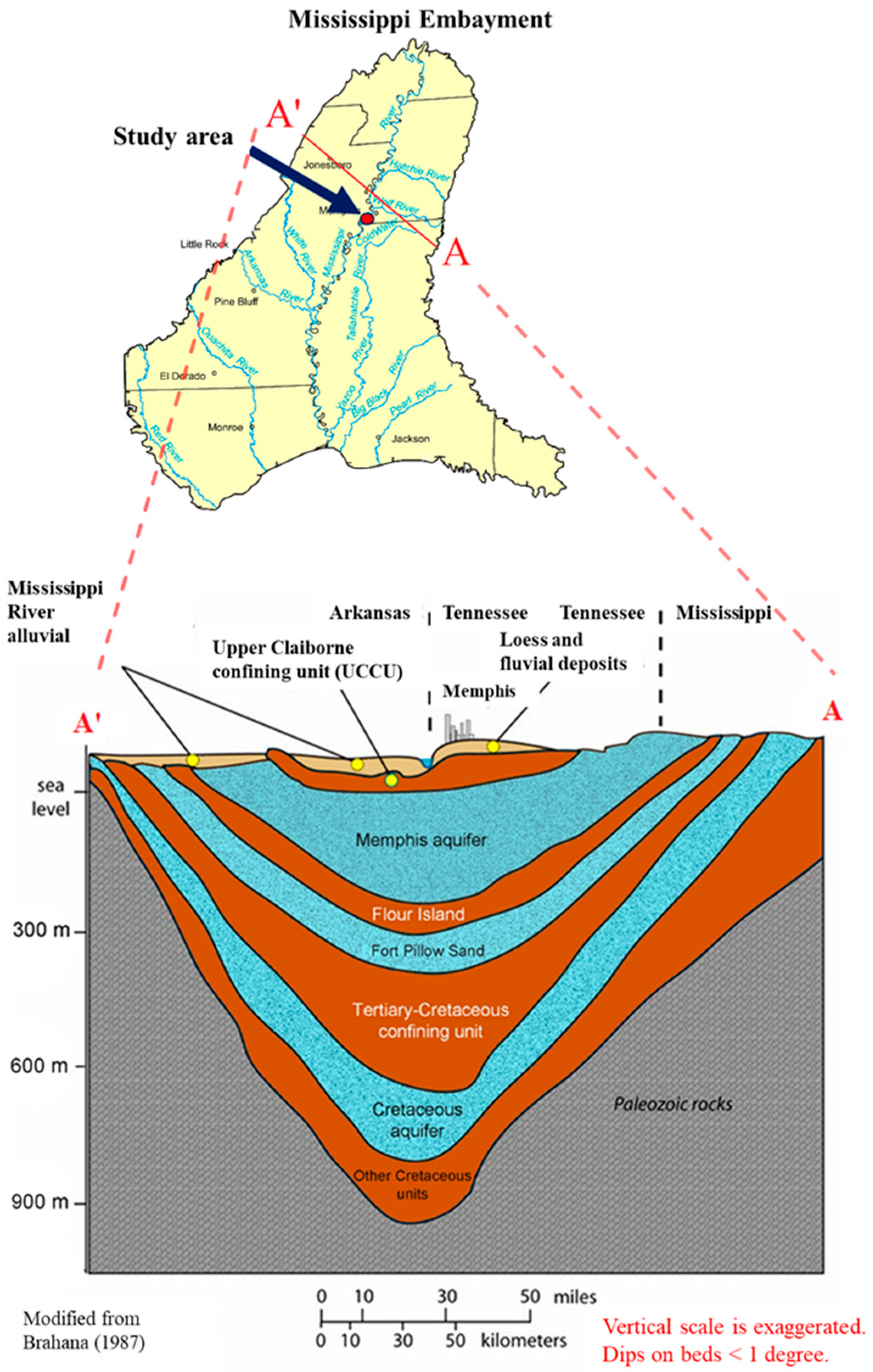
Memphis is within the Mississippi embayment aquifer system, and underlain by approximately one kilometer of unconsolidated sediments (Figure 1). The subsurface is divided into a series of alternating sand and clay layers, grouped into hydrostratigraphic units that include several water-bearing units. As shown in Figure 1, four sand aquifers beneath Shelby County, Tennessee include the Shallow aquifer, the Memphis aquifer, the Fort Pillow aquifer, and the Cretaceous aquifer, each of which are separated from adjacent aquifers by aquitard units, known as Upper Claiborne confining units (UCCU), Flour Island, Tertiary–Cretaceous confining unit, and other Cretaceous units [3,4]. The Shallow aquifer consists of the Mississippi River Valley alluvial (MRVA) aquifer, and the Gulf Coastal Plain (GCP) fluvial and alluvial aquifer. The MRVA aquifer serves as a water source for industrial, domestic, and irrigation wells in the Mississippi alluvial valley, and it is typically not utilized in urban settings. Water from the Shallow aquifer is of poorer quality than that in the underlying Memphis and Fort Pillow aquifers, due to the absence of an overlying aquitard; thus, it is locally contaminated in places. The Memphis aquifer serves as the primary source of drinking water in Shelby County, Tennessee, with minor withdrawals coming from the deeper Fort Pillow aquifer. However, the production well screened in the Fort Pillow aquifer is located in other cities (Cordova, and Millington) far from the City of Memphis. The Cretaceous aquifer is not utilized in Shelby County, due to the depth and poorer water quality.
The UCCU layer separates the Shallow and the Memphis aquifers throughout most of the Shelby County, acting as an upper protective layer to the Memphis aquifer. However, hydrogeologic breaches, also termed windows, within the UCCU locally create hydraulic connections between these aquifers [5]. The quantity of water passing through these hydraulic connections increases with greater groundwater withdrawal and groundwater head depression within the Memphis aquifer [6]. Hence, through these leaky hydrogeologic breaches where the hydraulic conductance is relatively high compared to the rest of the UCCU, the Shallow aquifer recharges the Memphis aquifer. Figure 2 demonstrates a schematic of a breach in the aquitard layer that acts as a preferential flow path from the Shallow aquifer to a screened production well in the Memphis aquifer.
Breaches in the UCCU aquitard threaten the water quality of the City of Memphis; therefore, identifying locations of the breaches are essential for source-water protection, and the development and implementation of wellhead protection plans. However, the seemingly straightforward question is—Where are the breaches? So far, two different approaches have been employed to answer this question. The first approach is the “geochemical investigation” [7,8,9,10,11,12,13] where groundwater samples are analyzed to identify geochemical signatures that are attributed to surface water within the groundwater. Within the Memphis area, age-dating of groundwater by using tritium-helium-3 and sulfur hexafluoride support geochemical data, and reflects the influence of modern water (<50 years) in the Memphis aquifer. Subsequent studies have shown that modern water contributes up to 40% of groundwater withdrawn from production wells—in one case, production water contains as much as 75% modern water [9,10,11]. The second approach is the “geological investigation”, in which techniques, such as surveying stratigraphic thickness and water table elevation, electrical resistivity surveys, shear-wave seismic reflection, and other geophysical analyses are used to identify gaps in impermeable layers [5,14,15,16,17]. Geological investigations show how hydrogeologic units are connected in the subsurface, and where preferential leakage pathways may exist. Parks [5] created an isopach map of the UCCU throughout Shelby County, and identified several areas where clay layers within the UCCU are thin or absent. Parks [5] also prepared a water-table elevation map for Shelby County, and showed that several areas with anomalous water-table depressions also had thin or absent confining unit clay, consistent with vertical leakage through a breach in the UCCU. Waldron et al. [16] used an S-wave seismic reflection survey to map the size and the orientation of localized breaches in the UCCU near an unlined landfill.
The abovementioned approaches have several limitations. First, mapping breaches are complicated, costly, and time-consuming owing to their depth, unknown location, and randomness of origin causality. Second, mapping studies with geophysical methods are technically limited to a small study area, and their measuring accuracy dissipates as the study area extends. Third, approaches involving extensive drilling and geophysical studies are inapplicable or prohibitive in urban areas, due to infrastructure, and compact residential and commercial areas. Therefore, when the presence of a breach in the aquitard layer is likely, numerical investigations conducted prior to field studies (pre-field investigation) can be extremely helpful to identify locations where a breach is likely to exist. Pre-field numerical investigations provide relevant and defensible explanations for groundwater flow anomalies in an aquifer system for informed decision-making.
Several numerical tools are developed to simulate the groundwater flow within the system. Groundwater models provide invaluable information about what cannot be adequately measured or observed, in both space and time domains (e.g., geological conceptualization, flow rates and flow pathways). Such numerical tools apply mathematical equations to calculate aquifer system responses to forcing conditions such as pumping, stream-stage variation, and rainfall events [18]. Besides groundwater models, several other numerical tools and techniques are developed to post-process the flow equations and the results of numerical models, to improve our understanding of the studied groundwater system [19,20,21,22,23,24,25,26,27].
In this work, we show how a combination of forward and backward numerical modeling, and post-processing numerical tools can be used to produce a more satisfactory representation of the groundwater system to make informed field investigation decisions. Herein, three numerical analyses are utilized: (1) pilot-point calibration analysis (PPC); (2) velocity and flow budget analyses (VFB); and (3) particle tracking analysis (PT), to reasonably identify the locations where the presence of breaches is likely. Finally, we test the results of each analysis against other evidence for breaches, to demonstrate that the results of the numerical analyses are reliable and supported by previous studies.
2. Methodology
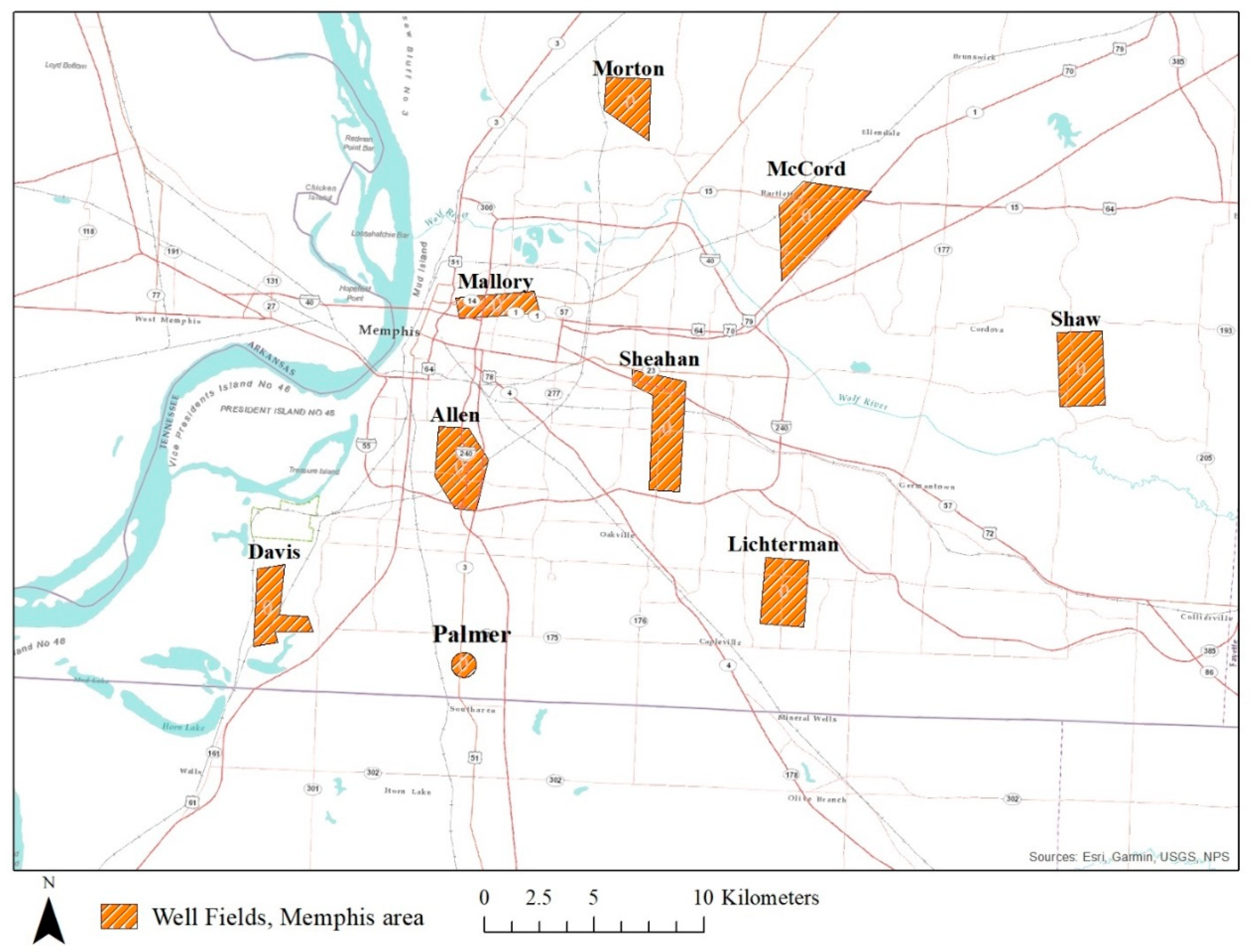
This study incorporates multiple Memphis Light, Gas and Water (MLGW) well fields, including the Allen, Davis, and Palmer well fields. These three well fields are located east of the Mississippi River bluff line in southwestern Shelby County (Figure 3), including 49 production wells (26 wells in Allen; 19 wells in Davis, and four wells in Palmer) and they collectively produce more than 50 million cubic meter per year over 2005 to 2016 [28]. Herein, we consider only the upper three geological units: (1) Shallow aquifer, (2) UCCU, and (3) Memphis aquifer (Figure 1). This approach is justified because all the production wells within the studying well fields are screened in the upper and middle Memphis aquifer, and little evidence exists for the upward flow of water from deeper hydrogeologic units [3]. Therefore, we neglect the interaction between the lower Memphis aquifer and the Flour Island aquitard, by assuming a no-flow boundary condition at the base of the Memphis aquifer (Figure 1).
2.1. Extent of the Study Area
In this study, we first assemble and analyze the existing relevant hydrogeological field data to define a proper extent for the study area, and we build an advisory conceptual model. In groundwater studies, the delineation of the extent of the study area is quite critical and challenging. To evaluate a proper extent for this study, we use the available potentiometric data of the Memphis aquifer in 2005, 2007, 2010 and 2015 [29,30]. Figure 4 shows the types and locations of boundary conditions that encompass Allen, Davis, and Palmer well fields. The purple, blue, green, and orange lines are associated with the years of 2005, 2007, 2010, and 2015, respectively. Dashed lines symbolize temporally varying boundary conditions in the Memphis aquifer (i.e., the groundwater heads along the dashed lines are spatially constant while their magnitudes vary with time). The solid line symbolizes the no-flow boundary condition at the groundwater divides between Allen, Sheahan, and Mallory well fields (Figure 3 and Figure 4). As shown in Figure 4, locations of both no-flow and temporarily varying boundary conditions remain nearly consistent from 2005 to 2015. Hence, we estimate the study area to encompass the average extent of the boundary conditions in different years, which is shown in black in Figure 4. The same extent is delineated for the Shallow aquifer and UCCU; however, with relevant spatially and temporally varying boundary conditions.
2.2. Conceptual Model
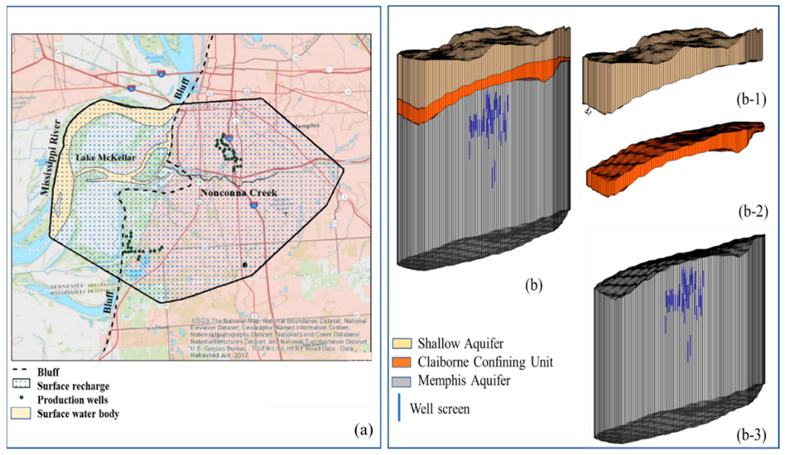
Figure 5 shows the conceptual model for the site-specific hydrogeological setting. In the conceptual model, we simplify the system conditions and capture the essential features of the site. Figure 5a shows a plan view of the conceptual model. A bluff line of 15 to 45 m high separates the alluvial and fluvial Shallow aquifers. Consequently, the hydraulic characteristics of the Shallow aquifer vary significantly on either side of the bluff line. Figure 5b shows a side view of the conceptual model which is made up of three layers: Shallow aquifer, UCCU, and the Memphis aquifer. Stratigraphic unit elevations were derived from [4]. Production well screen intervals are illustrated in Figure 5b, taking note that they vary in depth. This aquifer system conceptualization was very helpful in developing the numerical model.
2.3. Groundwater model
To describe the transient groundwater flow in the study area, we develop a high-resolution three-dimensional numerical model using [31]:
where h (L) is groundwater head, Kx, Ky, and Kz (L/T) are hydraulic conductivity in x, y, and z directions, respectively; t is time (T); S (1/L) is the storage coefficient of the aquifer and w (1/T) is a source and sink parameter (volumetric flux per unit volume). We used MODFLOW-NWT to solve Equation (1) [32]. The numerical model has six layers with a uniform m2 cells, totaling 20,773 active cells. The first and second numerical layers represent the Shallow aquifer and UCCU, respectively. The other four numerical layers uniformly divide the Memphis aquifer. The time domain of the model begins from 2005 to 2015, a span for which we have relatively sufficient data for Shallow and Memphis aquifer groundwater head within the study area. This duration is discretized into 121 monthly stress periods, each subdivided into five smaller time steps.
2.4. Initial Conditions and Boundary Conditions
In this study, the initial head conditions of the Shallow aquifer were set to the water-table surface (Shallow aquifer) as measured in 2005. There was no information available regarding the groundwater head in UCCU. Therefore, we assumed the same initial conditions within the UCCU in 2005 [33]. The initial head conditions for the Memphis aquifer were derived from the 2005 Memphis aquifer potentiometric surface [30]. Boundary conditions of the Shallow aquifer, UCCU, and Memphis aquifer were estimated using available potentiometric surfaces from 2005 to 2015. The boundary condition of the Shallow aquifer was assumed to be spatially and temporally varying during 2005–2015, except beneath the Mississippi River, where it is controlled by the river stage variations. Therefore, the boundary condition under the Mississippi River is estimated according to the monthly measurements of river stage at the nearby Beale Street gage during the period of 2005 to 2015 [34]. We neglected the horizontal inflow and outflow at the UCCU boundary condition; therefore, the boundary condition of the UCCU was assumed to be a no-flow boundary condition. Two boundary conditions were applied to the Memphis aquifer: no-flow (which is perpendicular to equipotential lines) and temporarily varying boundary conditions (Figure 3). The Memphis aquifer head variation at the varying boundary condition, at many points, remained within a relatively small range of fluctuation during 2005 to 2015. Therefore, the temporally varying boundary condition of the Memphis aquifer was estimated by interpolating available 2005 to 2015 Memphis aquifer heads [30].
2.5. Internal Forcing Conditions
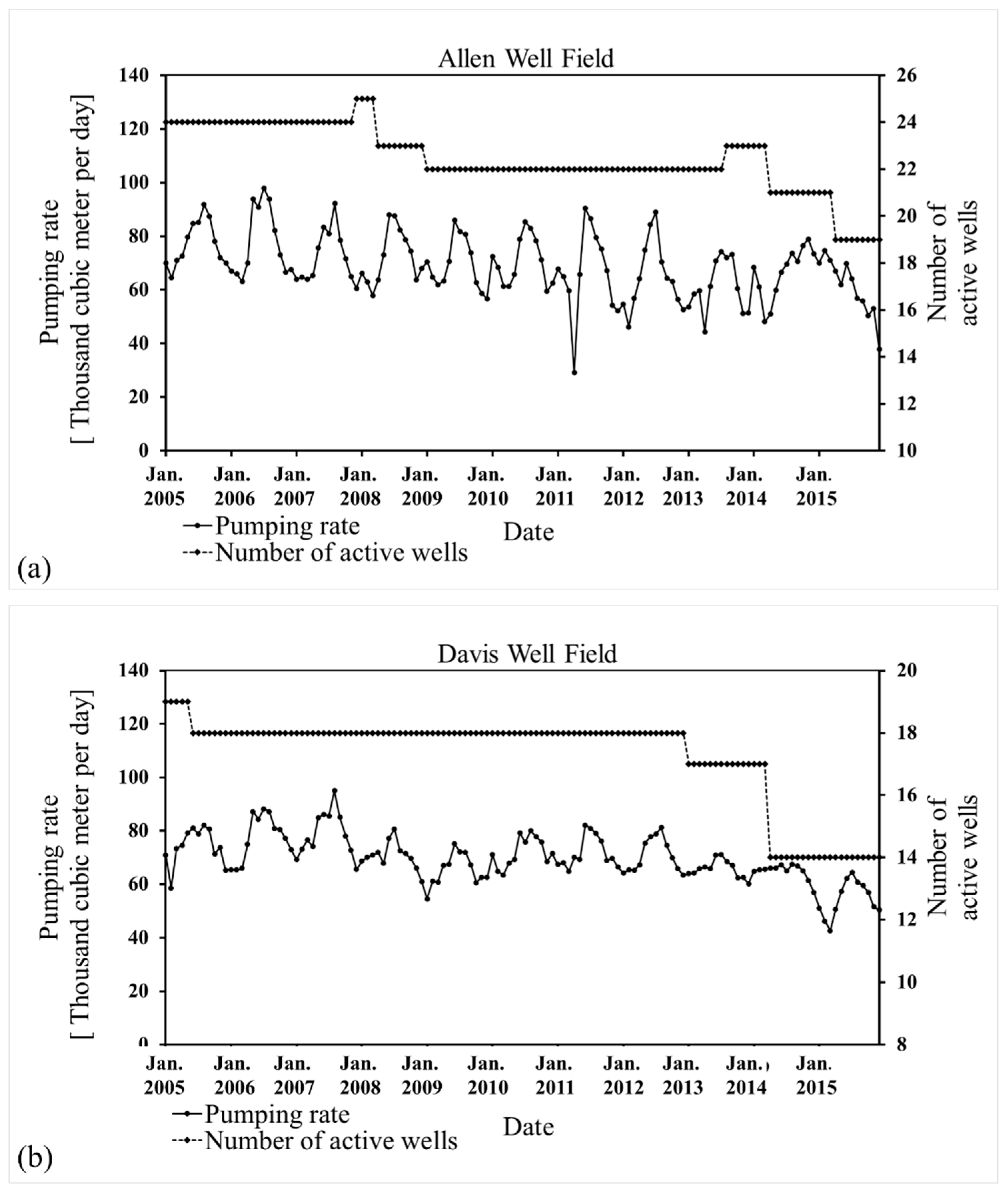
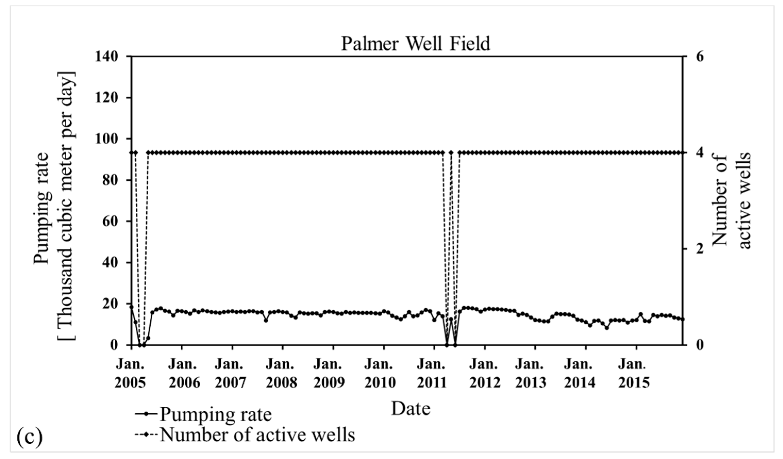
Internal forcing conditions within the study area included McKellar Lake, Nonconnah Creek, production wells, and surface recharge. Since McKellar Lake has an open connection to the Mississippi River, the lake stage follows Mississippi River stages. The Nonconnah Creek stage variation was modeled using monthly mean stages measured at upstream and downstream stations, Farris View Drive stage and Riverport stage, during the period 2011 to 2017, when the stage data were recorded (Rivergages.com, 2018). The exact withdrawal rates of the production wells are unavailable. Therefore, monthly production for the entire well fields are uniformly distributed to each active well during that month [34]. The pumping rates of each well field and the number of active wells in each month are shown in Figure 6a–c. Precipitation recharge was applied to the upper layer, representing the Shallow aquifer surface recharge. Unfortunately, recharge rates to the shallow aquifer are unknown, and they must be inferred from available precipitation records. However, since precipitation events occur almost in all months of each year in the study area [35] we assumed a temporarily constant recharge rate over the modelling time domain and a spatially varying recharge rate over the study area (See Appendix C). Finally, the recharge rates will be estimated during model calibration processes.
3. Numerical Analysis Results
In this study, we located zones where the presence of leaky aquitard (UCCU) breaches was likely, by applying three numerical analyses: (1) PPC performed against horizontal and vertical hydraulic conductivities, (2) VFB, and (3) PT. As it pertains the identifying plausible aquitard breach locations, the following observances were assumed: (1) hydraulic conductivities at breaches were expected to be locally high, (2) convergence of flow to a specific area was a sign of the presence of a breach, and (3) vertical flow at breaches was expectedly high, compared with other parts of the study area. These conditions will be derived from the PPC and VFB. In contrast, PT should show that groundwater particles at the breaches vertically transport further than in the surrounding area.
3.1. Pilot Point Calibration Analyses (PPC)
Although the boundary conditions and withdrawal rates were estimated, several parameters required for groundwater modeling, including horizontal and vertical hydraulic conductivities, storage coefficients, surface recharge, and the conductance of the hyporheic zone at Nonconnah Creek bed were remain unknown. To estimate the unknowns, we used an advanced nonlinear method of spatial parameter characterization to develop an inverse groundwater model [36]. An inverse groundwater model includes a calibration process to achieve a satisfactory fit between the model predictions and field measurements. However, most of the time, the solution to the groundwater problem is inherently non-unique [36,37,38]. Based on the groundwater literature, one would address the non-uniqueness issue by introducing additional “simplifying” information such as the use of zonal calibration, in which the model is subdivided into a limited number of zones with constant parameter values [39]. The values of parameters in each zone can be restricted to a range that is estimated from the actual field data. Furthermore, additional information can be introduced to the model through advanced mathematical regularization in the parameter calibration process, like truncated singular value decomposition (SVD) [36,37,38,40]. Finally, like all predicting models, the model predictions are required to fit the collected observation data, and to produce reasonable results, based on previous knowledge of the system. In this study, we used all of the abovementioned techniques to address the challenging non-uniqueness issue.
We first used uniform properties for each layer to estimate proper starting calibration values within a meaningful range of parameters, as reported in previous studies conducted in the Mississippi embayment area [3,39,41,42,43,44,45,46]. In the groundwater literature, this approach is known as zonal calibration [47,48]. We considered two zones at the east and west of the bluff for Shallow aquifer. Similarly, we considered two zones at either side of the bluff for UCCU. Finally, we considered one zone for each numerical layer (four layers) of the Memphis aquifer. The range of parameters estimated in previous studies within and outside of the study area are summarized in Table 1. However, it should be noted that inherent uncertainty exists in the estimated data, due to the limited number of estimations, and due to the different test protocols [49,50]. This type of uncertainty increases with depth, especially in the Memphis aquifer, which needs to be considered during modeling and calibration.
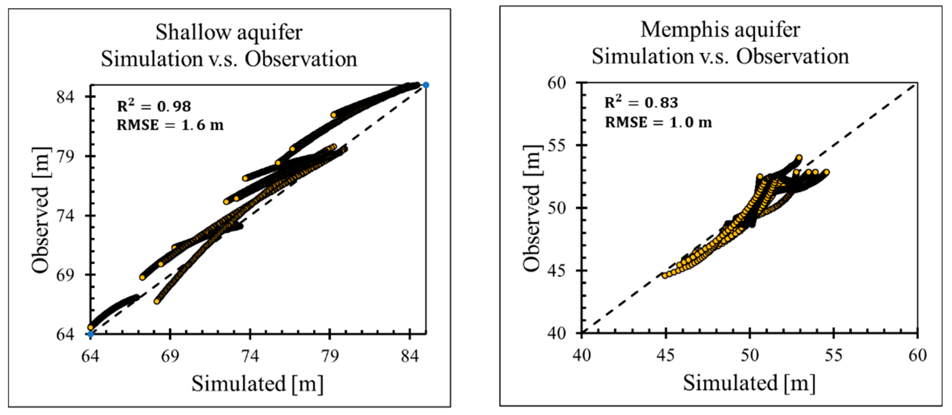
Parameters used for this pre-calibration process were horizontal and vertical hydraulic conductivities, storage coefficients, the Nonconnah Creek bed conductance, and surface recharge. To describe the heterogeneity in hydraulic conductivity and surface recharge within each zone, we used “pilot points” accompanied by advanced singular value decomposition (SVD) regularization functionality available through PEST [36,37]. This model included 69 pilot points distributed in all layers. The inverse distance weighted method is used to spatially distribute pilot points values to each cell of the model. We used PEST to estimate a new set of the model parameters (i.e., horizontal and vertical hydraulic conductivities, storage coefficients, the Nonconnah Creek bed conductance, and surface recharge) using a robust mathematical technique by comparing simulation results to a set of observations [36,37]. Observation points were derived from the available Shallow and Memphis aquifers potentiometric surfaces maps [30,33]. To evaluate the calibration results, we compared the simulated transient groundwater head with the observed data at 23 observation points within the Shallow and Memphis aquifers. Shallow aquifer observation data included water levels collected in 2005 and 2015. The Memphis aquifer observation data included groundwater heads collected during 2005 to 2015. Groundwater head fluctuation in each observation point was not high; therefore, the monthly varying head at each observation point was estimated by linear interpolation between the years for when the observation data were available. To evaluate the goodness of calibration, the observed and simulated groundwater heads were compared with each other. The observed versus simulated groundwater heads are shown in Figure 7. The goodness-of-fit coefficients between the simulated and calibrated results of the model were computed for all observation points within the Shallow and the Memphis aquifers [51]. values of Shallow and Memphis aquifers were estimated to be 0.98 and 0.84, respectively. Root Mean Square Error (RMSE) values of Shallow and Memphis aquifers were estimated to be 1.6 m and 1.0 m, respectively. The estimated and RMSE indicated a satisfactory goodness of fit.
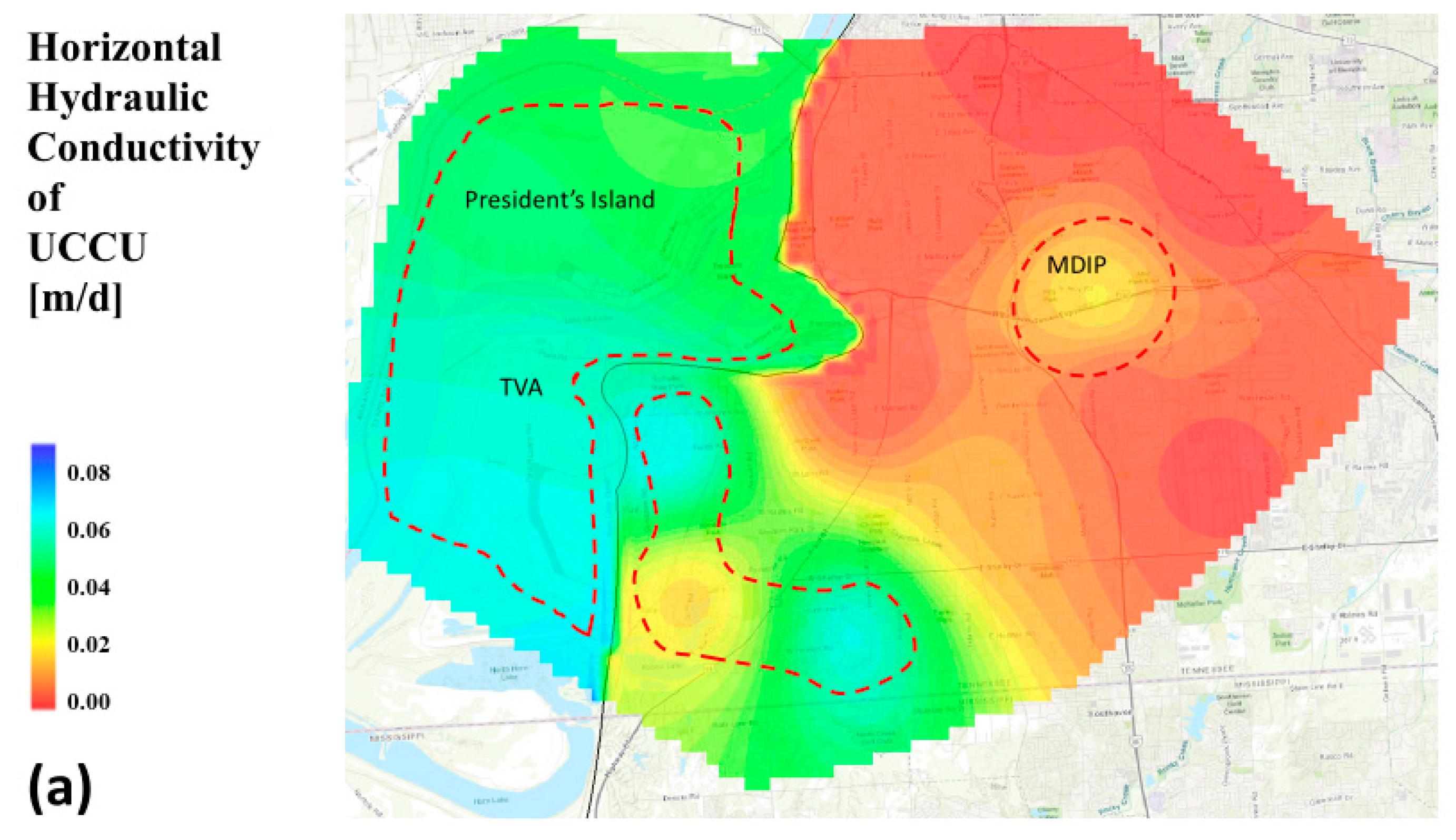
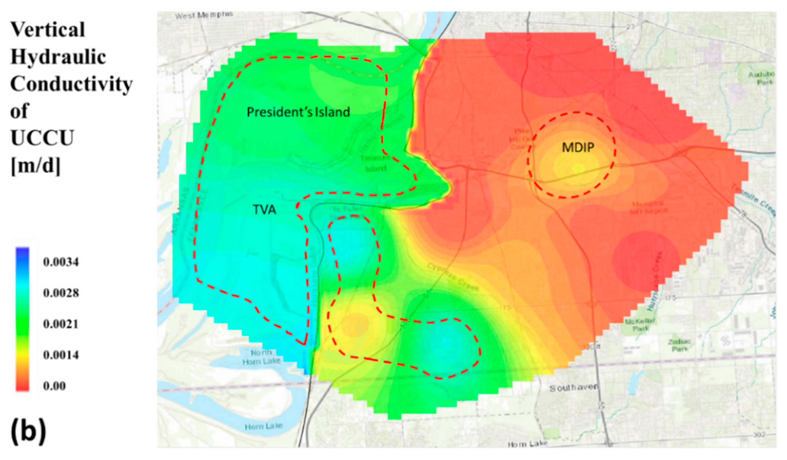
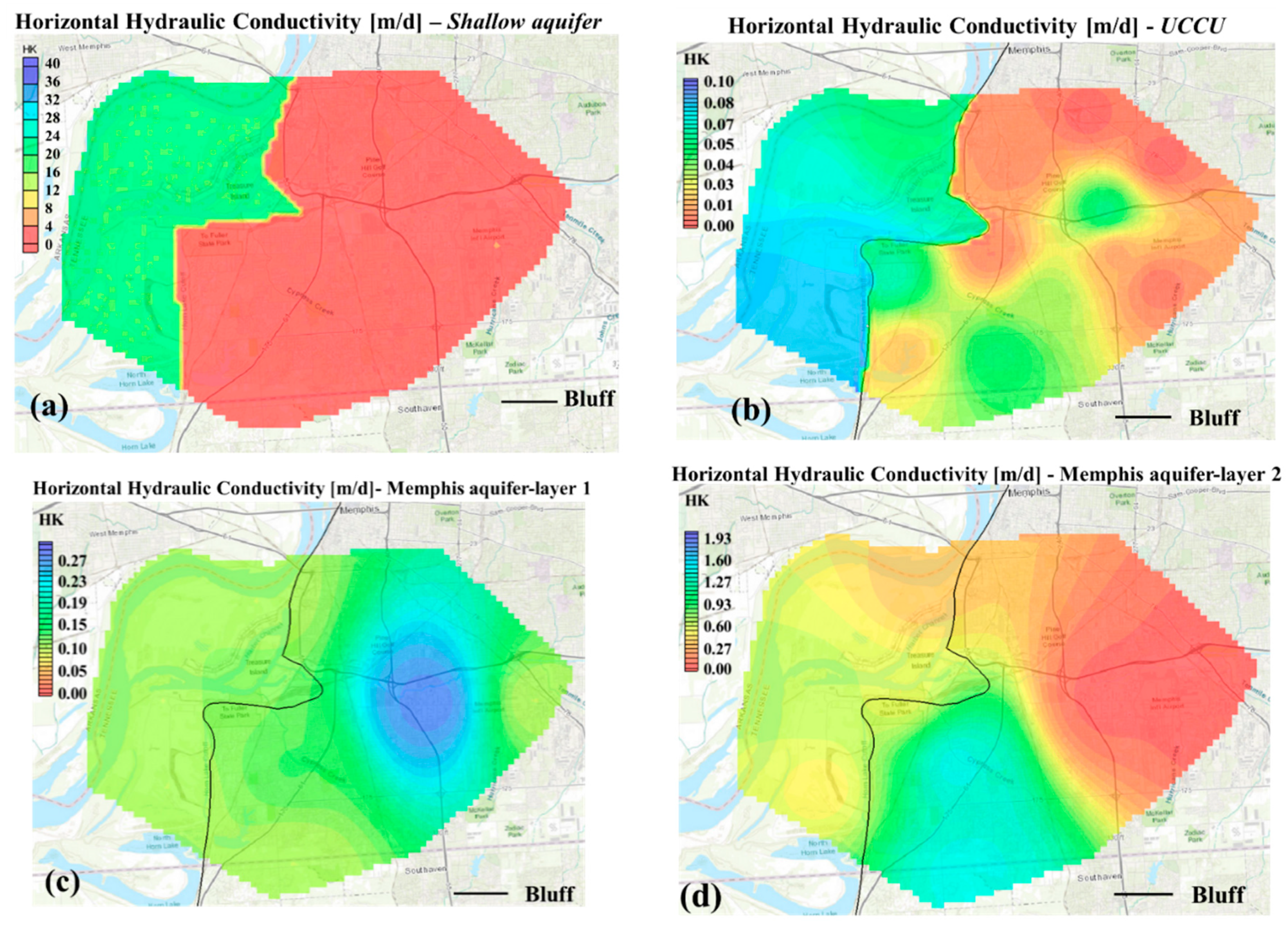
The calibrated horizontal and vertical hydraulic conductivities of the UCCU are shown in Figure 8a,b, respectively. Figure 8 shows that the patterns of the distribution of horizontal and vertical hydraulic conductivities were quite similar, however, with different values (see Appendixe A, Appendixe B and Appendixe C which summarize all six numerical layers’ calibrated hydraulic conductivities, storage coefficients, and surface recharge, respectively). As shown in Figure 8, PPC revealed three major zones (dashed lines) in which the vertical and horizontal hydraulic conductivities of the UCCU were relatively high. Since we expected locally high hydraulic conductivities at the breaches, we concluded that the presence of the breaches at these three zones were more probable than other parts of the study area.
3.2. Validation of PPC Results
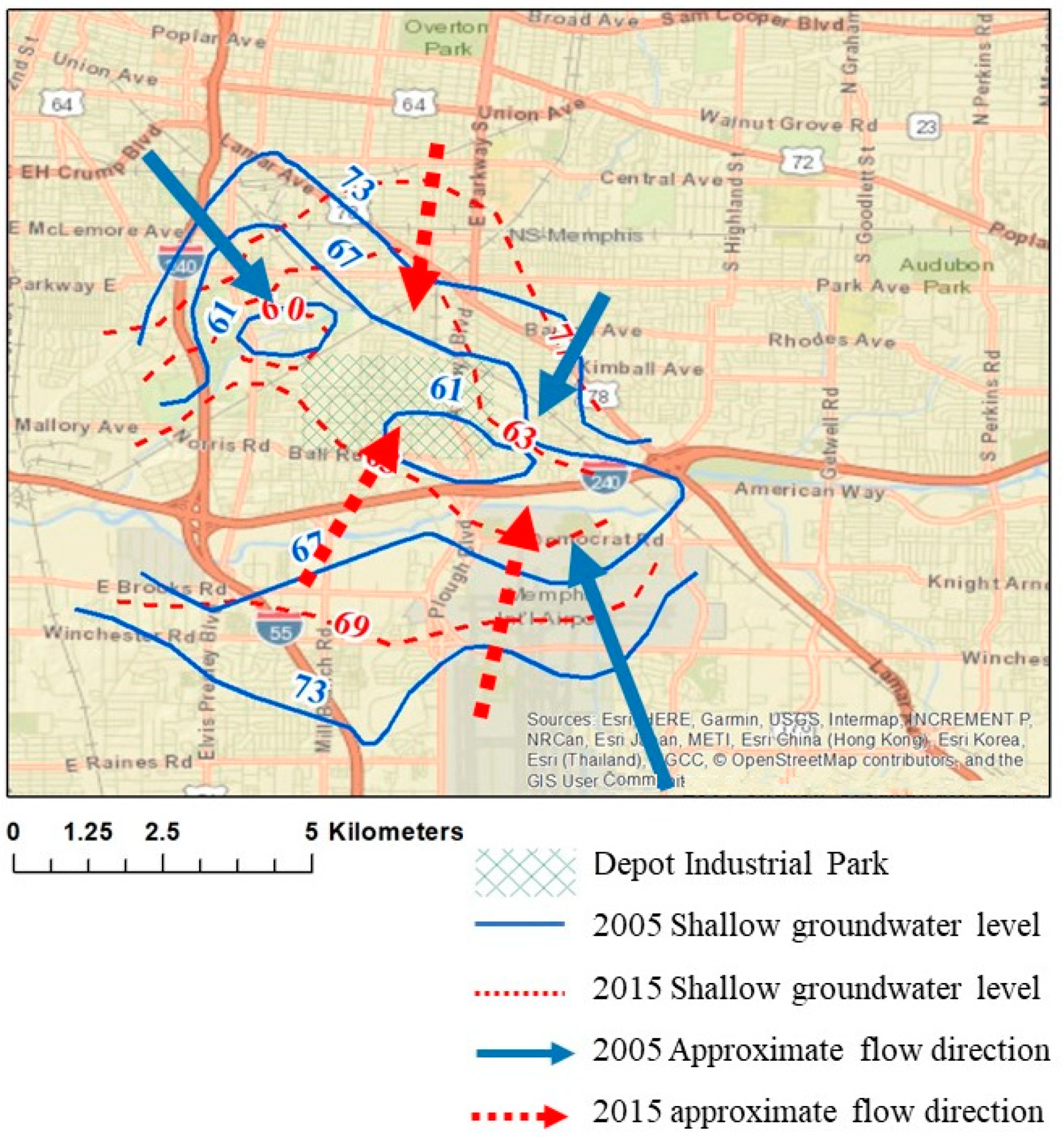
The increase of hydraulic conductivities represented within the three identified zones (Figure 8) likely exist due to lithologic variation or erosion of the UCCU, with an increase of coarser grained sediments [52,53]. The first identified area by PPC is located in the Memphis Depot Industrial Park (MDIP) (Figure 8). Recent investigations have already indicated that the Shallow groundwater level in this area is locally lower than that in the surrounding areas [33,54]. Figure 9 shows the approximate flow directions of Shallow aquifer in 2005 and 2015, which converge from the surrounding areas toward the MDIP. There are no pumping wells in this area, which otherwise would have resulted in a local cone of depression.
The second zone is located on President’s Island (Figure 8). Previous studies and field investigation in this area have indicated that the thickness of the UCCU beneath President’s Island significantly thins [41]. Calibration results in the President’s Island area affirm the suspicion of the thinning or absence of the UCCU. Moreover, in the area immediately south of President’s Island, which includes the Tennessee Valley Authority (TVA) combined cycle plant, a hydraulic connection of the Shallow and Memphis aquifer is identified [54] (Figure 8). This recent study supports the likely presence of a breach in that area.
The third identified zone is located at the southern part of the study area adjacent to the bluff line. This area is an undiscovered zone, where field investigations are lacking. Therefore, this area is considered as an area of interest, where further investigations are required to validate the PPC results.
3.3. Velocity and Flow Budget Analyses (VFB)
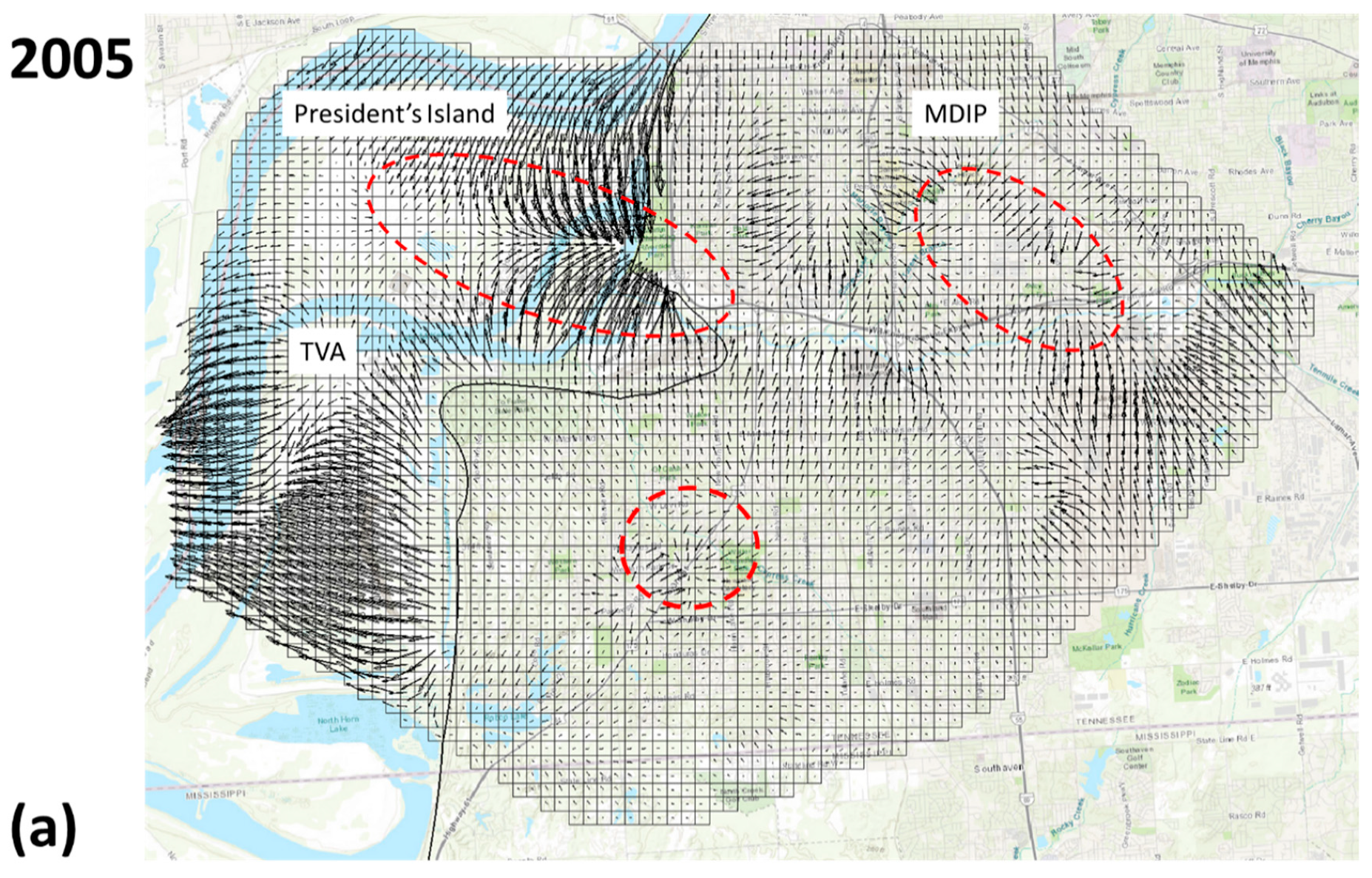
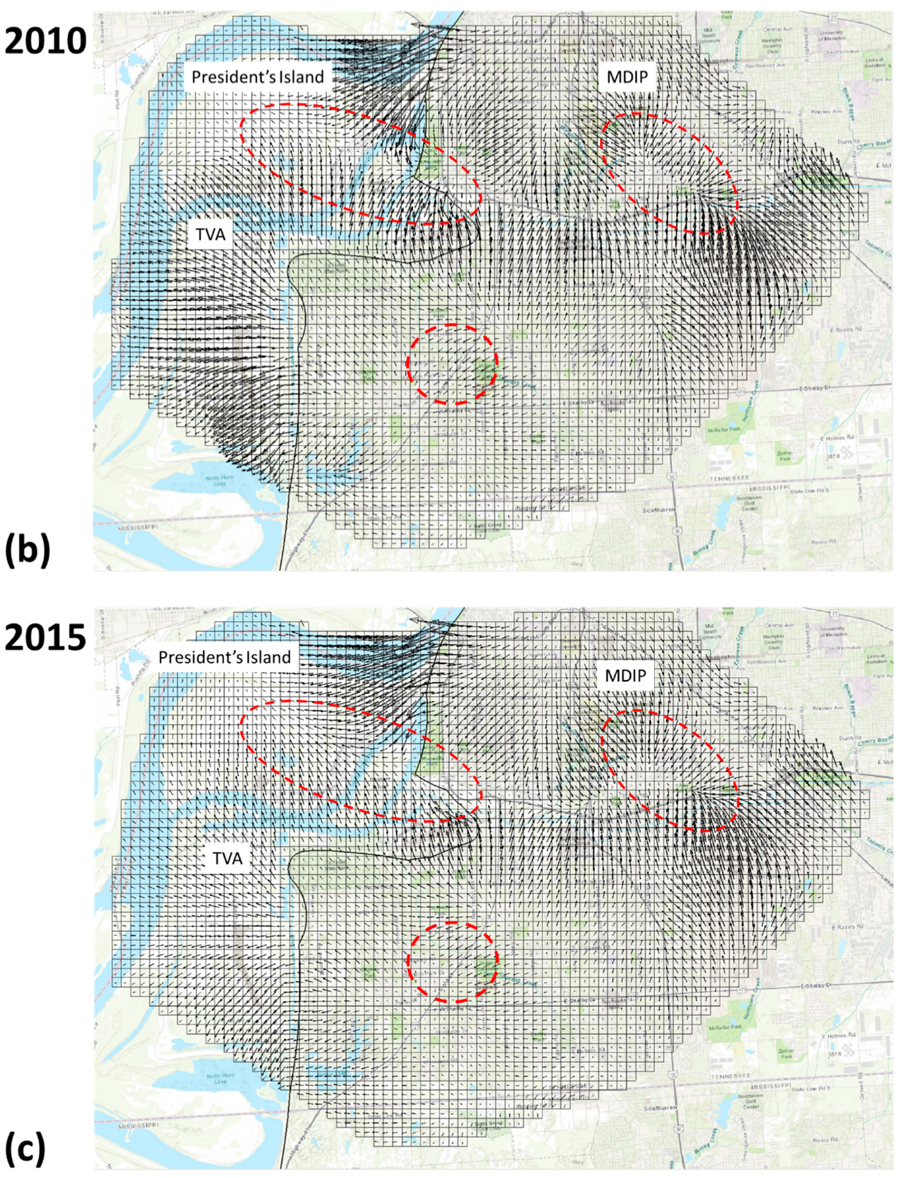
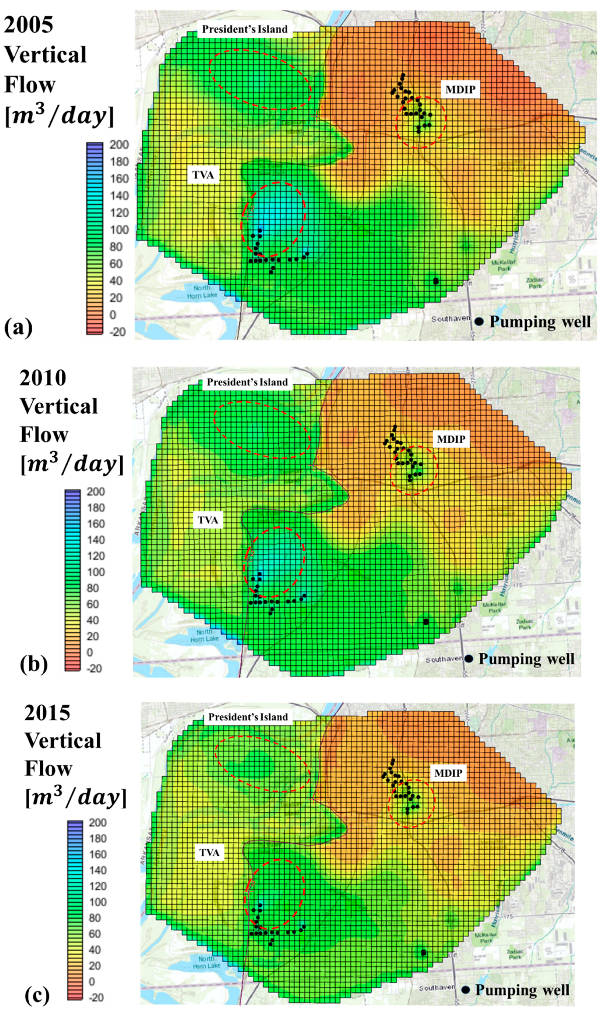
High hydraulic conductivity alone at a breach does not necessarily lead to a vertical flow, and it needs sufficient vertical gradient to create flow. Determining the velocity and flow directions of the Shallow aquifer can provide valuable information regarding the likely presence of a breach. Figure 10a–c shows the horizontal velocity vector of the Shallow aquifer in the study area in 2005, 2010, and 2015 derived from the developed numerical model. The magnitude of the velocity is proportional to the arrows lengths. A longer arrow refers to a higher horizontal velocity. As shown in Figure 10a–c, the VFB approach identified three zones where the velocity vectors converged to specific areas. The horizontal velocity of groundwater decreases inside the convergence zones, suggesting downward flow (assuming upward flow is negligible due to the regional downward vertical gradient). As shown in Figure 11a–c, VFB analyses also show vertical downward flow budgets at the bottom of the Shallow aquifer in 2005, 2010, and 2015, respectively. Negative values refer to an upward flow, and positive values refer to a downward flow. As shown in Figure 11a–c, the vertical flows in all three identified zones by VFB are locally high. Figure 11a–c shows a weak correlation between the extent and location of the identified zones, and the extent and location of the production wells (note that all wells are screened within the Memphis aquifer). It might be because the UCCU weakens the influence of wells on the vertical flow of the Shallow aquifer. Therefore, it can be concluded that the local increase in the vertical flow of the shallow aquifer is not associated with the production wells. The main difference between the results of the PPC and VFB analyses is that VFB did not show any local flow convergence and an increase in vertical flow budget at the TVA area. Using this approach, we can conclude that the presence of breaches at the three identified zones is more likely than other parts of the study area.
3.4. Validation of VFB Results
As shown in Figure 10, the velocity vectors converge and focalize to three specific zones where the vertical flow of the shallow aquifer is locally high, as shown in Figure 11. These zones are almost the same as the three zones identified by PPC analysis, except in the TVA area; therefore, VFB analysis only verifies the previous findings in the MDIP and President’s Island. However, it should be noted that VFB identifies smaller breach areas, compared with PPC. The third identified zone at the southern part of the study area is an undiscovered zone, where further local and detailed investigations are required for verification. It should be noted that the convergence of the flow near the Nonconnah Creek is not necessarily, because of the presence of a breach in this area. Flow budget analysis shows that the convergence of the flow in this area is mainly because of the drainage of the Shallow aquifer to the creek.
3.5. Particle Tracking Analyses (PT)
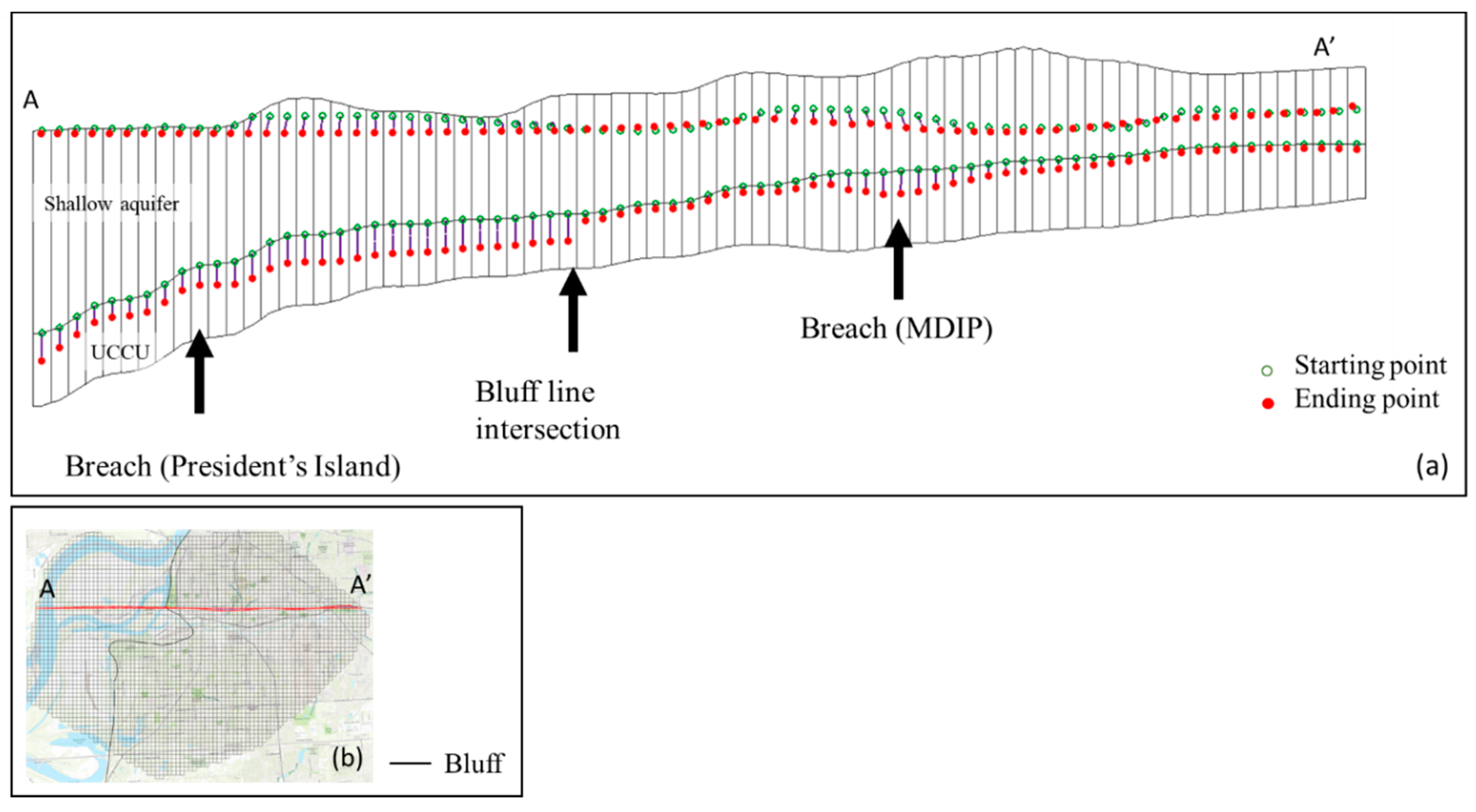
In this approach, we used the numerical tool, MODPATH [20], to conduct forward particle tracking. Figure 12a shows the cross-section A-A’ of the Shallow aquifer and UCCU, an east-to-west transect of the study area that is shown in context in Figure 12b. Forward particle tracking represents the location of imaginary particles at the Shallow aquifer surface, and at the top of the UCCU from 2005 (green marks) to 2015 (red marks). Figure 12a shows the vertical downward flow transport from the Shallow aquifer and UCCU to the Memphis aquifer. A sudden change was observed at the bluff line, due to differences in alluvial (west of the bluff) and fluvial (east of the bluff) deposits characteristics. The particles in the MDIP area also locally penetrated further from 2005 to 2015. As shown, particles west of the bluff within the President’s Island moved downward significantly faster than the east of the bluff, consistent with the higher hydraulic conductivity of the MRVA and fluvial deposits at either side of the bluff line.
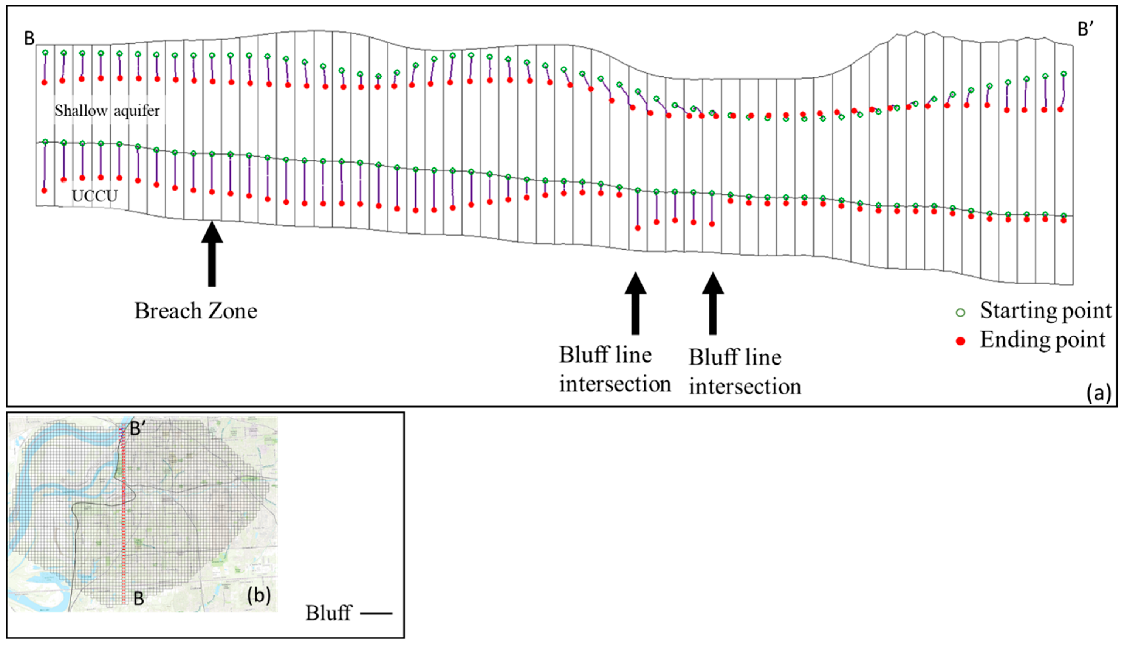
Figure 13a shows placement of north–south cross-section B–B’ of the Shallow aquifer and UCCU, which are shown in context in Figure 13b. Cross-section B–B’ intersects the bluff at three points. Figure 13a shows a sudden change in particle migration proximal to the bluff, due to hydraulic characteristics differences in alluvial and fluvial deposits at either side of the bluff line. Particles at the southern part of the cross-section B–B’ transport further at depth from 2005 to 2015, compared with particles at the northern part of the cross-section.
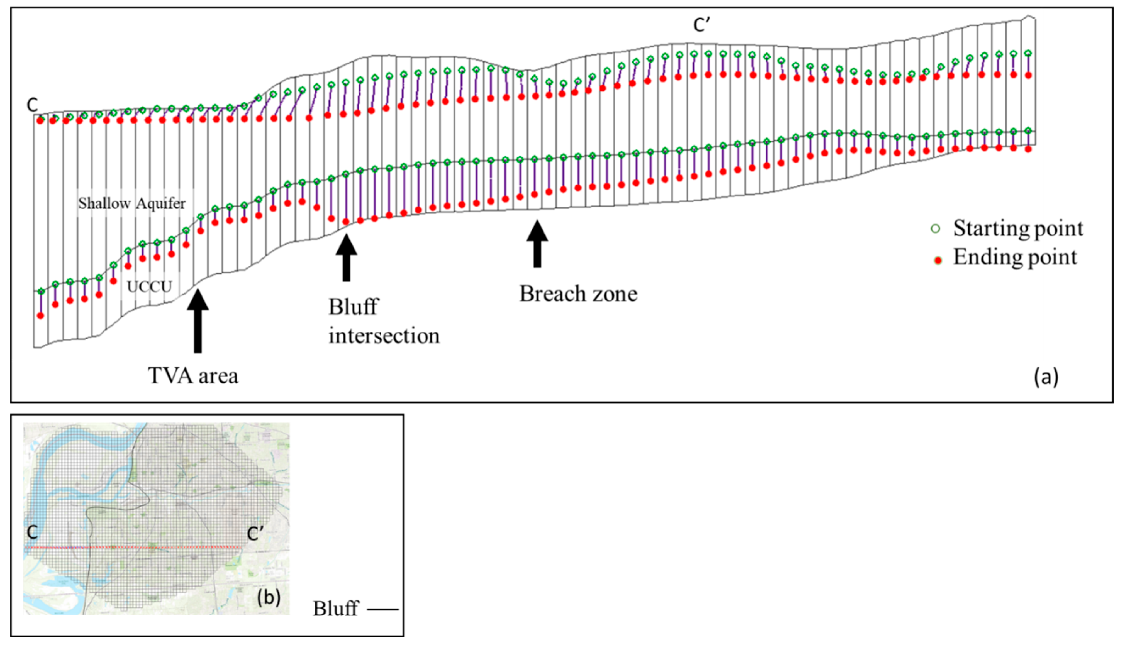
Figure 14a shows the cross-section C–C’ of the Shallow aquifer and UCCU, an east-to-west transect of the study area that is shown in context in Figure 14b. The cross-section intersects the bluff at one point. Similarly, we place imaginary particles on the Shallow aquifer and top of UCCU in the year of 2005 (green marks). Forward particle tracking represents the location of each particle in 2015 (red marks). Same as in cross-section A–A’, an abrupt change is observed at the bluff; however, PPT results show a relatively high interaction between the layers adjacent the bluff line. As shown in Figure 14a, PPT shows no sign of a breach at the TVA area. However, there is a broad area east of the bluff where particles transport paths are relatively long. Therefore, there is a high possibility for the presence of a breach in this area.
3.6. Validation of PT Results
PT results confirmed all the zones identified by PPC and VFB analyses. The results show that the particles in the President’s Island and MDIP transport locally further, which is consistent with previous studies [14,34,54] in these areas. PT shows that particles in the TVA area transport slowly downward, except adjacent to the bluff line. This finding is consistent with a recent study [54]. However, similar to PPC analysis, there is an undiscovered area in the southern part of the study area where PT identifies it as the locations where the presence of breaches is likely.
4. Summary and Conclusions
The Memphis aquifer is the primary drinking water source in the Shelby County (Tennessee, USA), and it supplies industrial, commercial, and residential water. Memphis aquifer is one of several deep-sand aquifers separated from the Shallow aquifer by a clayey confining layer, UCCU. All of the production wells in the Memphis area are screened in the Memphis aquifer or even deeper in Fort Pillow aquifer, to avoid Shallow aquifer contamination. Traditionally, the public water supply authority in the Memphis area assumed that the UCCU could fully protect the water in the Memphis aquifer from downward leakage of the contaminated or poor-quality groundwater from the overlying Shallow aquifer. However, recent studies show that at some locations, the UCCU is thin or absent, which leads to the contribution of water from the Shallow aquifer to the Memphis aquifer [9,10,11,14]. Hence, sustainable water management in the Memphis area requires the locations of breaches in the UCCU to ensure the protection of water pumped from the production wells. Locating breaches demands expensive geological or geochemical investigations. These studies are even more costly and complicated in densely developed urban areas. Therefore, other techniques are desired that can help to determine the locations of breaches, so that complicated and costly field investigations can be focused in limited areas.
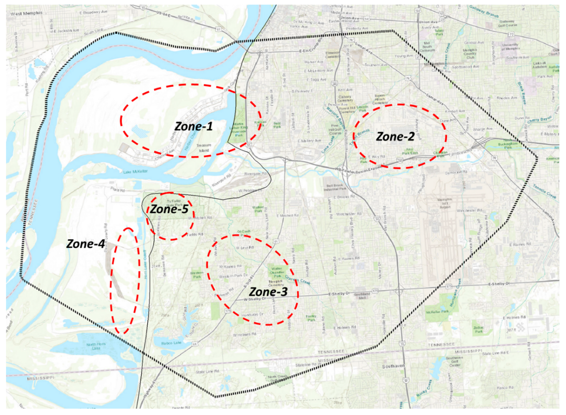
In this study, to identify the locations where the presence of breaches in the UCCU is likely, we use three different analyses: (1) pilot point calibration (PPC), (2) velocity and flow budget (VFB), and (3) particle tracking (PT). As shown in Figure 15, these approaches identify five zones where the presence of breaches is expected. As summarized in Table 2, all three approaches distinguish Zones 1, 2, and 3 from other parts of the study area. However, VFB does not identify Zones 4 and 5 as the locations of possible breaches. Previous investigations results are concurrent with this study, in that the presence of breaches in Zone 1, 2, and 4 is likely. These findings validate the reliability of the numerical model. However, the presence of breaches in Zones 3 and 5 have never been explored, and they need further investigation. Five zones identified in this study are reasonable candidates for future field investigations, based on the current understanding of the study area. The results of this study can reduce the cost and increase the efficiency of investigations all over the broad study area, by directing future studies.
In this study, we show how a numerical pre-field investigation can tackle complex hydrogeological problems. A similar approach and analyses that have been developed in this work can be applied to study the interaction between the geological layers of an aquifer, provided that enough information about the boundary conditions, hydraulic properties, and geologic characteristics are available. As in all numerical models, the consistency, stability, and accuracy of the model depends on the quantity and quality of the available data. Gathering hydraulic and geologic data is costly and time-consuming, and it usually needs several years to fulfill. This study is an example of reliable models that have been built on information collected over several years.
Author Contributions
Authors collaborated together for the completion of this work and jointly conceived the idea. Farhad Jazaei conducted modeling, developed the first draft of this manuscript, and wrote the manuscript. Brian Waldron, Scott Schoefernacker, Daniel Larsen reviewed the paper and provided useful ideas to improve the work.
Funding
This work was fully funded by Memphis Light, Gas, and Water (MLGW) Division grant under the title of Allen Wellfield Evaluation (Contract#11783).
Conflicts of Interest
The authors declare no conflict of interest.
Appendix A
Figure A1.
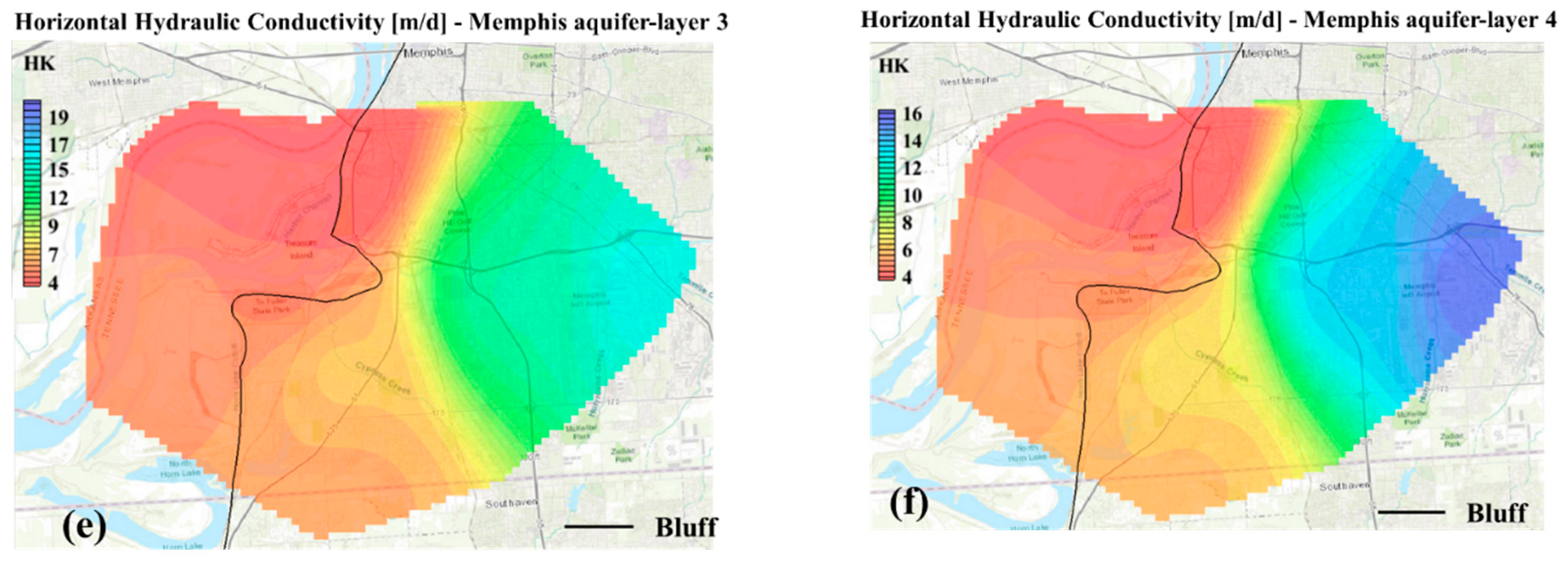
(a–f) The horizontal hydraulic conductivities of each numerical layer.


Figure A2.
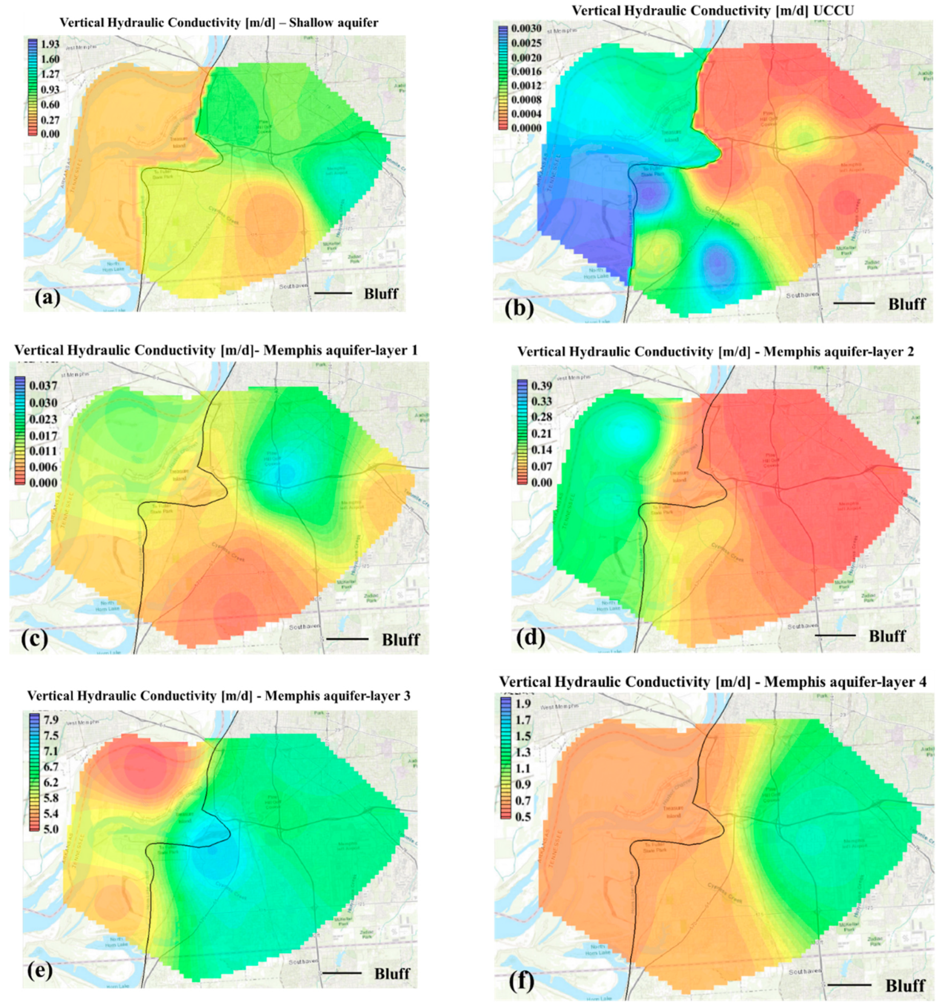
(a–f) The vertical hydraulic conductivities of each numerical layer.

Appendix B
Figure A3.
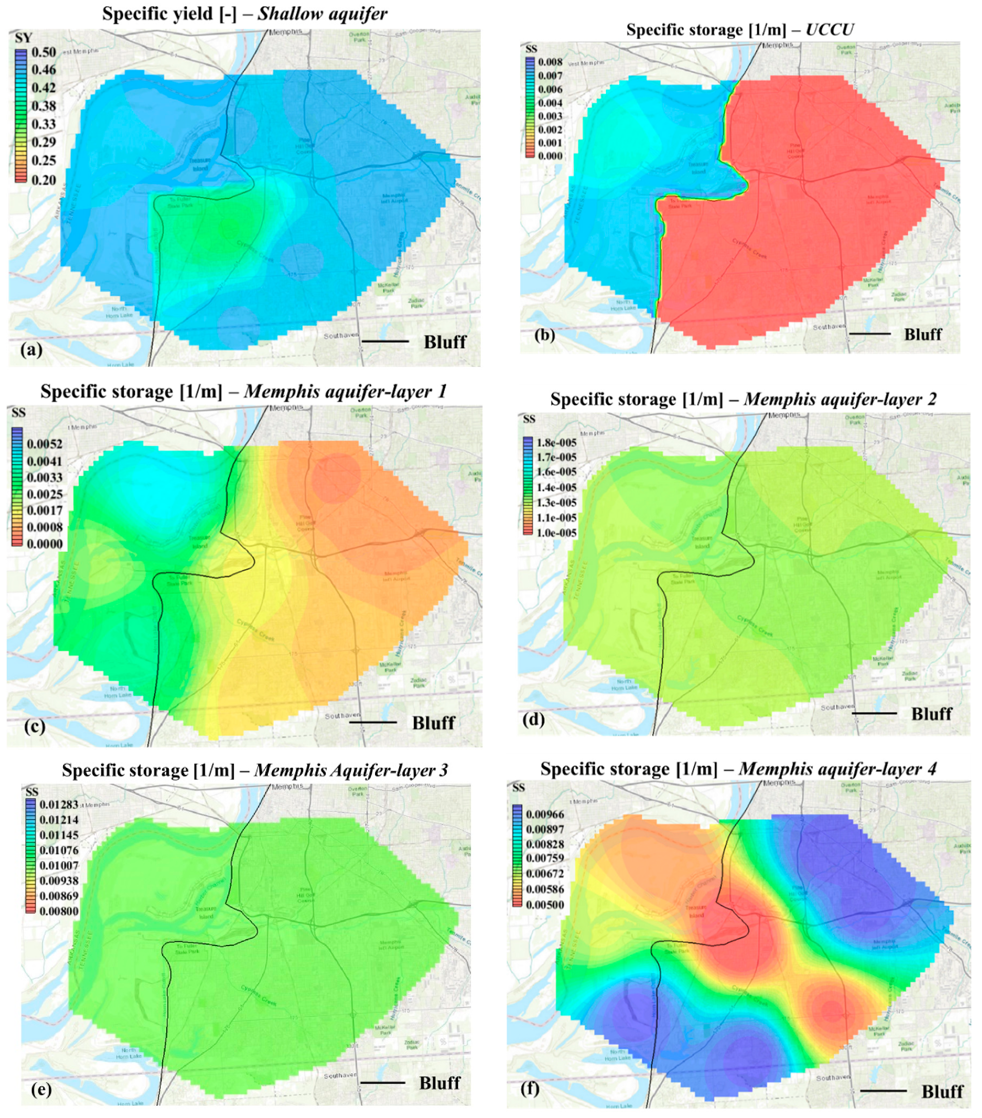
(a) The specific yield coefficient of the Shallow aquifer. (b–f) The specific storage of UCCU and Memphis aquifer, respectively.
Figure A3.
(a) The specific yield coefficient of the Shallow aquifer. (b–f) The specific storage of UCCU and Memphis aquifer, respectively.

Appendix C
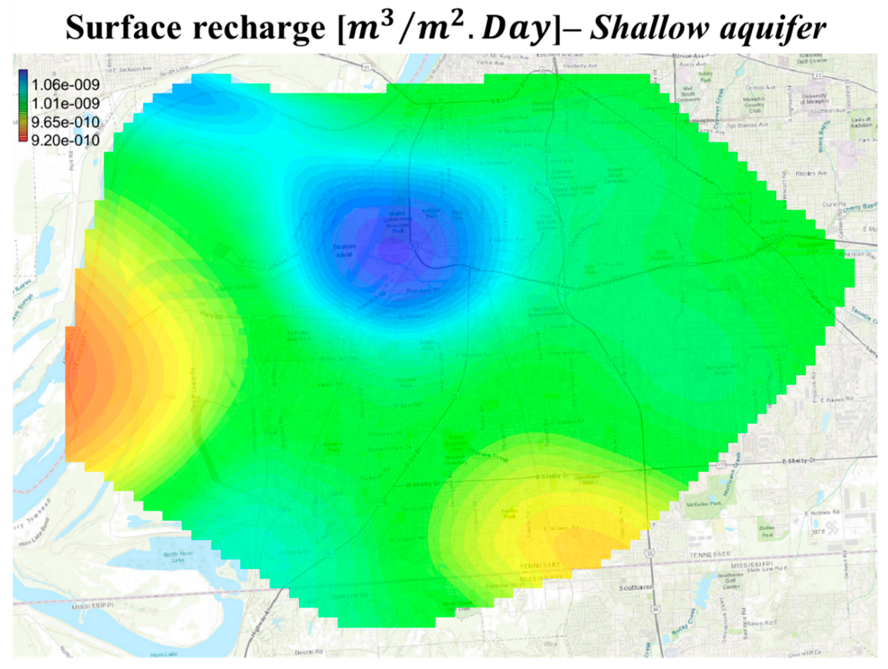
Figure A4.
The calibrated surface recharge to the Shallow aquifer.

References
- Dieter, C.A.; Maupin, M.A.; Caldwell, R.R.; Harris, M.A.; Ivahnenko, T.I.; Lovelace, J.K.; Barber, N.L.; Linsey, K.S. Estimated Use of Water in the United States in 2015; US Geological Survey: Tallahassee, FL, USA, 2018.
- Sparks, J.W. Industry Focus: Water Resources—Greater Memphis, 100 Trillion Gallons. Available online: https://businessfacilities.com/2015/06/industry-focus-water-resources-greater-memphis-100-trillion-gallons/ (accessed on 21 August 2018).
- Brahana, J.V.; Broshears, R.E. Hydrogeology and Ground-Water Flow in the Memphis and Fort Pillow Aquifers in the Memphis Area, Tennessee. 2001. Available online: https://pubs.usgs.gov/wri/wri894131/pdf/text_wri89-4131_1.pdf (accessed on 20 December 2018).
- Clark, B.R.; Hart, R.M. The Mississippi Embayment Regional Aquifer Study (MERAS): Documentation of a Groundwater-Flow Model Constructed to Assess Water Availability in the Mississippi Embayment; US Geological Survey: Tallahassee, FL, USA, 2009.
- Parks, W.S. Hydrogeology and Preliminary Assessment of the Potential for Contamination of the Memphis Aquifer in the Memphis Area, Tennessee; US Geological Survey: Tallahassee, FL, USA, 1990.
- Kingsbury, J.A.; Parks, W.S. Hydrogeology of the Principal Aquifers and Relation of Faults to Interaquifer Leakage in the Memphis Area, Tennessee; US Department of the Interior, US Geological Survey: Washington, DC, USA, 1993.
- Neretnieks, I. Age dating of groundwater in fissured rock: Influence of water volume in micropores. Water Resour. Res. 1981, 17, 421–422. [Google Scholar] [CrossRef]
- Busenberg, E.; Weeks, E.P.; Plummer, L.N.; Bartholomay, R.C. Age dating ground water by use of chlorofluorocarbons (CCl3F and CCl2F2), and distribution of chlorofluorocarbons in the unsaturated zone, Snake River plain aquifer, Idaho National Engineering Laboratory, Idaho. In USGS Water Resources Investigations Report; US Geological Survey: Tallahassee, FL, USA, 1993. [Google Scholar]
- Larsen, D.; Gentry, R.W.; Solomon, D.K. The geochemistry and mixing of leakage in a semi-confined aquifer at a municipal well field, Memphis, Tennessee, USA. Appl. Geochem. 2003, 18, 1043–1063. [Google Scholar] [CrossRef]
- Larsen, D.; Morat, J.; Waldron, B.; Ivey, S.; Anderson, J. Stream Loss Contributions to a Municipal Water Supply Aquifer in Memphis, Tennessee. Environ. Eng. Geosci. 2013, 19, 265–287. [Google Scholar] [CrossRef]
- Larsen, D.; Waldron, B.; Schoefernacker, S.; Gallo, H.; Koban, J.; Bradshaw, E. Application of Environmental Tracers in the Memphis Aquifer and Implication for Sustainability of Groundwater Resources in the Memphis Metropolitan Area, Tennessee. J. Contemp. Water Res. Educ. 2016, 159, 78–104. [Google Scholar] [CrossRef] [Green Version]
- Ivey, S.S.; Gentry, R.W.; Larsen, D.; Anderson, J. Inverse Application of Age-Distribution Modeling Using Environmental Tracers H 3/ He 3. J. Hydrol. Eng. 2008, 13, 1002–1010. [Google Scholar] [CrossRef]
- Majidzadeh, H.; Uzun, H.; Ruecker, A.; Miller, D.; Vernon, J.; Zhang, H.; Bao, S.; Tsui, M.T.; Karanfil, T.; Chow, A.T. Extreme flooding mobilized dissolved organic matter from coastal forested wetlands. Biogeochemistry 2017, 136, 293–309. [Google Scholar] [CrossRef]
- Besson, A.; Cousin, I.; Samouëlian, A.; Boizard, H.; Richard, G. Structural heterogeneity of the soil tilled layer as characterized by 2D electrical resistivity surveying. Soil Tillage Res. 2004, 79, 239–249. [Google Scholar] [CrossRef]
- Waldron, B.A.; Harris, J.B.; Larsen, D.; Pell, A. Mapping an aquitard breach using shear-wave seismic reflection. Hydrogeol. J. 2009, 17, 505–517. [Google Scholar] [CrossRef]
- Schoefernacker, S. Evaluation and Evolution of a Groundwater Contaminant Plume at the Former Shelby County Landfill, Memphis, Tennessee. Ph.D. Thesis, The University of Memphis, Memphis, TN, USA, 2018. [Google Scholar]
- Anderson, M.P.; Woessner, W.W.; Hunt, R.J. Applied Groundwater Modeling: Simulation of Flow and Advective Transport; Academic Press: San Diego, CA, USA, 2015. [Google Scholar]
- Pollock, D.W. User’s Guide for MODPATH/MODPATH-PLOT, Version 3: A Particle Tracking Post-Processing Package for MODFLOW, the US: Geological Survey Finite-Difference Ground-Water Flow Model. 1994. Available online: https://pubs.usgs.gov/of/1994/0464/report.pdf (accessed on 20 December 2018).
- Owen, S.J.; Jones, N.L.; Holland, J.P. A comprehensive modeling environment for the simulation of groundwater flow and transport. Eng. Comput. 1996, 12, 235–242. [Google Scholar] [CrossRef]
- Zimmerman, D.A.; de Marsily, G.; Gotway, C.A.; Marietta, M.G.; Axness, C.L.; Beauheim, R.L.; Bras, R.L.; Carrera, J.; Dagan, G.; Davies, P.B. A comparison of seven geostatistically based inverse approaches to estimate transmissivities for modeling advective transport by groundwater flow. Water Resour. Res. 1998, 34, 1373–1413. [Google Scholar] [CrossRef] [Green Version]
- Van Dam, J.C.; Feddes, R.A. Numerical simulation of infiltration, evaporation and shallow groundwater levels with the Richards equation. J. Hydrol. 2000, 233, 72–85. [Google Scholar] [CrossRef]
- Guha, H. A stochastic modeling approach to address hydrogeologic uncertainties in modeling wellhead protection boundaries in karst aquifers. JAWRA J. Am. Water Resour. Assoc. 2008, 44, 654–662. [Google Scholar] [CrossRef]
- Simpson, M.J.; Jazaei, F.; Clement, T.P. How long does it take for aquifer recharge or aquifer discharge processes to reach steady state? J. Hydrol. 2013, 501, 241–248. [Google Scholar] [CrossRef]
- Jazaei, F.; Simpson, M.J.; Clement, T.P. An analytical framework for quantifying aquifer response time scales associated with transient boundary conditions. J. Hydrol. 2014, 519, 1642–1648. [Google Scholar] [CrossRef]
- Jazaei, F.; Simpson, M.J.; Clement, T.P. Spatial analysis of aquifer response times for radial flow processes: Nondimensional analysis and laboratory-scale tests. J. Hydrol. 2016, 532, 1–8. [Google Scholar] [CrossRef] [Green Version]
- Jazaei, F.; Simpson, M.J.; Clement, T.P. Understanding time scales of diffusive fluxes and the implication for steady state and steady shape conditions. Geophys. Res. Lett. 2017, 44, 174–180. [Google Scholar] [CrossRef]
- Upon Request: TDEC Dataviewers. Available online: https://www.tn.gov/environment/about-tdec/tdec-dataviewers.html (accessed on 21 August 2018).
- USGS Water Data for the Nation. Available online: https://waterdata.usgs.gov/nwis? (accessed on 22 August 2018).
- Kingsbury, J.A. Altitude of the Potentiometric Surface, 2000–15, and Historical Water-Level Changes in the Memphis Aquifer in the Memphis Area, Tennessee (USGS Numbered Series No. 3415), Scientific Investigations Map; US Geological Survey: Tallahassee, FL, USA, 2018.
- Bear, J. Hydraulics of Groundwater; McGraw-Hill: New York, NY, USA, 1979. [Google Scholar]
- Niswonger, R.G.; Panday, S.; Ibaraki, M. MODFLOW-NWT, a Newton formulation for MODFLOW-2005. US Geol. Surv. Tech. Methods 2011, 6, 44. [Google Scholar]
- Narsimha, V.K. Altitudes of Ground Water Levels for 2005 and Historic Water Level Change in Surficial and Memphis Aquifers, Shelby County, Tennessee. Master’s Thesis, University of Memphis, Memphis, TN, USA, 2007. [Google Scholar]
- Rivergages.com: Providing River Gage Data for Rivers, Streams and Tributaries. Available online: http://rivergages.mvr.usace.army.mil/WaterControl/new/layout.cfm (accessed on 21 June 2018).
- U.S. Climate Data. Available online: https://www.usclimatedata.com/climate/memphis/tennessee/united-states/ustn0325 (accessed on 21 August 2018).
- Doherty, J. Ground water model calibration using pilot points and regularization. Groundwater 2003, 41, 170–177. [Google Scholar] [CrossRef]
- Doherty, J. Manual for PEST: Model-Independent Parameter Estimation Manual, 5th ed.; Watermark Numerical Computing: Brisbane, Australia, 2002.
- Moore, C.; Doherty, J. The cost of uniqueness in groundwater model calibration. Adv. Water Resour. 2006, 29, 605–623. [Google Scholar] [CrossRef]
- Doherty, J.; Hunt, R.J. Two statistics for evaluating parameter identifiability and error reduction. J. Hydrol. 2009, 366, 119–127. [Google Scholar] [CrossRef]
- Graham, D.D.; Parks, W.S. Potential for Leakage among Principal Aquifers in the Memphis Area, Tennessee (Vol. 85, No. 4295); US Department of the Interior, US Geological Survey: Washington, DC, USA, 1986.
- Moore, G.K. Geology and Hydrology of the Claiborne Group in Western Tennessee. US Government Printing Office, 1965. Available online: https://pubs.usgs.gov/wsp/1809f/report.pdf (accessed on 20 December 2018).
- Parks, W.S.; Carmichael, J.K. Geology and Ground-Water Resources of the Cockfield Formation in Western Tennessee (Vol. 88, No. 4181); US Department of the Interior, US Geological Survey: Washington, DC, USA, 1990.
- Parks, W.S.; Carmichael, J.K. Geology and Ground-Water Resources of the Fort Pillow Sand in Western Tennessee; US Department of the Interior, US Geological Survey: Washington, DC, USA, 1989.
- Carmichael, J.K.; Parks, W.S.; Kingsbury, J.A.; Ladd, D.E. Hydrogeology and Ground-Water Quality at Naval Support Activity Memphis, Millington, Tennessee; US Geological Survey Water Resources Investigation; 1997. Available online: https://pubs.usgs.gov/wri/1997/4158/report.pdf (accessed on 20 December 2018).
- Robinson, J.L.; Carmichael, J.K.; Halford, K.J.; Ladd, D.E. Hydrogeologic framework and simulation of ground-water flow and travel time in the shallow aquifer system in the area of Naval Support Activity Memphis, Millington, Tennessee. In US Geological Survey Water-Resources Investigations Report; US Geological Survey: Washington, DC, USA, 1997. [Google Scholar]
- Gentry, R.W.; Ku, T.L.; Luo, S.; Todd, V.; Larsen, D.; McCarthy, J. Resolving aquifer behavior near a focused recharge feature based upon synoptic wellfield hydrogeochemical tracer results. J. Hydrol. 2006, 323, 387–403. [Google Scholar] [CrossRef]
- Park, C.; Seo, J.; Lee, J.; Ha, K.; Koo, M.-H. A distributed water balance approach to groundwater recharge estimation for Jeju volcanic island, Korea. Geosci. J. 2014, 18, 193–207. [Google Scholar] [CrossRef]
- Jiménez, S.; Mariethoz, G.; Brauchler, R.; Bayer, P. Smart pilot points using reversible-jump Markov-chain Monte Carlo. Water Resour. Res. 2016, 52, 3966–3983. [Google Scholar] [CrossRef]
- Waldron, B.; Larsen, D.; Hannigan, R.; Csontos, R.; Anderson, J.; Dowling, C.; Bouldin, J. Mississippi embayment regional ground water study. In United States Environmental Protection Agency Publication 600/R-10/130; US EPA: Washington, DC, USA, 2011. [Google Scholar]
- Villalpando-Vizcaino, R. Development of a Numerical Multi-Layered Groundwater Model to Simulate Inter-Aquifer Water Exchange in Shelby County, Tennessee. Master’s Thesis, University of Memphis, Memphis, TN, USA, 2018. [Google Scholar]
- Glantz, S.A.; Slinker, B.K.; Neilands, T.B. Primer of Applied Regression and Analysis of Variance; McGraw-Hill Education: New York, NY, USA, 1990. [Google Scholar]
- Ebina, T.; Minja, R.J.; Nagase, T.; Onodera, Y.; Chatterjee, A. Correlation of hydraulic conductivity of clay–sand compacted specimens with clay properties. Appl. Clay Sci. 2004, 26, 3–12. [Google Scholar] [CrossRef]
- Alakayleh, Z.; Clement, T.P.; Fang, X. Understanding the Changes in Hydraulic Conductivity Values of Coarse-and Fine-Grained Porous Media Mixtures. Water 2018, 10, 313. [Google Scholar] [CrossRef]
- Bradshaw, E.A. Assessment of Ground-Water Leakage through the Upper Claiborne Confining Unit to the Memphis Aquifer in the Allen Well Field, Memphis, Tennessee. Ph.D. Thesis, University of Memphis, Memphis, TN, USA, 2011. [Google Scholar]
- Carmichael, J.K.; Kingsbury, J.A.; Larsen, D.; Schoefernacker, S. Preliminary Evaluation of the Hydrogeology and Groundwater Quality of the Mississippi River Valley Alluvial Aquifer and Memphis Aquifer at the Tennessee Valley Authority Allen Power Plants, Memphis, Shelby County, Tennessee; US Geological Survey: Washington, DC, USA, 2018.
Figure 1.
A–A’ hydrogeological section of the Memphis groundwater system, through the Mississippi Embayment. It represents four aquifers and four confining units. Note that the vertical axis is dramatically exaggerated for visualization purposes. The study area is shown as a red circle in the Mississippi Embayment map.

Figure 2.
The methods by which pollution can be transferred from urban activities to the Shallow aquifer, and finally to the Memphis aquifer, through a breach.
Figure 2.
The methods by which pollution can be transferred from urban activities to the Shallow aquifer, and finally to the Memphis aquifer, through a breach.

Figure 3.
All active well fields in the Memphis area.

Figure 4.
The no-flow boundary condition (solid lines) and temporarily varying boundary conditions (dashed lines) of the Memphis aquifer for the years of 2005, 2007, 2010, and 2015. The black line shows the estimated extent of the study area.
Figure 4.
The no-flow boundary condition (solid lines) and temporarily varying boundary conditions (dashed lines) of the Memphis aquifer for the years of 2005, 2007, 2010, and 2015. The black line shows the estimated extent of the study area.

Figure 5.
(a) A plan view of the conceptual model that includes a part of the Mississippi River, McKellar Lake, Nonconnah Creek, production wells, and surface recharge. (b) A side view of the conceptual model, and the location of production well screens. (b-1), (b-2), and (b-3) separately show the Shallow aquifer, UCCU, and the Memphis aquifer, respectively.

Figure 6.
(a–c) shows the pumping rates and the number of active wells of Allen, Davis, and Palmer well fields from 2005 to 2015 in each month, respectively.
Figure 6.
(a–c) shows the pumping rates and the number of active wells of Allen, Davis, and Palmer well fields from 2005 to 2015 in each month, respectively.


Figure 7.
(a,b) show observed vs simulated results of the model for the Shallow and Memphis aquifers, respectively.
Figure 7.
(a,b) show observed vs simulated results of the model for the Shallow and Memphis aquifers, respectively.

Figure 8.
(a,b) maps show calibrated horizontal and vertical hydraulic conductivities of UCCU, respectively. They show relatively higher hydraulic conductivities in three zones: Memphis Depot Industrial Park (MDIP), Tennessee Valley Authority (TVA), and President’s Island, and the south of the study area.


Figure 9.
A map of the Shallow aquifer groundwater level, and approximate flow directions in 2005 (blue arrow) and 2015 (red arrow) at the MDIP area.
Figure 9.
A map of the Shallow aquifer groundwater level, and approximate flow directions in 2005 (blue arrow) and 2015 (red arrow) at the MDIP area.

Figure 10.
(a–c) maps show the Shallow aquifer groundwater velocity vectors for 2005, 2010, and 2015, respectively. The magnitudes of the velocities are proportional to the length of the arrows. Three zones where the groundwater velocity vectors are converged are shown. The presence of a breach in these zones are more probable than that of the surrounding areas.


Figure 11.
(a–c) maps show vertical flow budgets at the bottom of the Shallow aquifer in 2005, 2010, and 2015, respectively. Negative values refer to upward flow, and positive values refer to downward flows.
Figure 11.
(a–c) maps show vertical flow budgets at the bottom of the Shallow aquifer in 2005, 2010, and 2015, respectively. Negative values refer to upward flow, and positive values refer to downward flows.

Figure 12.
The A–A’ cross section of the Shallow aquifer, and the UCCU used for particle tracking. (a) shows the Shallow aquifer and the UCCU at the cross section. (b) shows the plan view of the cross section. Particles are placed on top of the groundwater in the shallow aquifer, and on top of the UCCU in 2005 (Green mark). Forward particle tracking shows the transport of the particles within the layers (blue line), and the position of each particle at the end of simulation in 2015 (Red mark).

Figure 13.
B–B’ cross section of the shallow aquifer and the UCCU, showing particle tracking results. (a) shows cross-section of the shallow aquifer and the UCCU along B–B’. (b) shows the plan view of the cross section. Particles are placed on top of the groundwater in the shallow aquifer, and on top of the UCCU, in 2005 (green mark). Forward particle tracking shows the transport of the particles within the layers (blue line), and the position of each particle at the end of the simulation in 2015 (red mark).

Figure 14.
C–C’ cross section of the shallow aquifer and the UCCU, showing particle tracking results. (a) shows cross-section of the shallow aquifer and the UCCU along C–C’. (b) shows the plan view of the cross section. Particles are placed on top of the groundwater in the shallow aquifer and top of the UCCU in the year of 2005 (green mark). Forward particle tracking shows the transport of the particles in the layers (blue line), and the position of each particle at the end of simulation in 2015 (red mark).

Figure 15.
Five zones identified by pilot-point calibration (PPC), velocity and flow budget (VFB), and particle tracking (PT) where further field investigations are required.
Figure 15.
Five zones identified by pilot-point calibration (PPC), velocity and flow budget (VFB), and particle tracking (PT) where further field investigations are required.


Table 1.
Minimum and maximum of hydraulic parameters reported in previous studies within and nearby the study area [3,39,41,42,43,44,45,46].
| Minimum | Maximum | |||||||
|---|---|---|---|---|---|---|---|---|
| Horizontal hydraulic conductivity (m/d) | Vertical hydraulic conductivity (m/d) | Storage coefficients (1/m) | Specific yield (-) | Horizontal hydraulic conductivity (m/d) | Vertical hydraulic conductivity (m/d) | Storage coefficients (1/m) | Specific yield (-) | |
| Shallow aquifer - East of the bluff | 1 | 2.60 × 10⁻⁵ | - | 0.22 | 46 | 7.00 × 10⁻¹ | - | 0.48 |
| Shallow aquifer - West of the bluff | 36 | - | - | 0.28 * | 119 | - | - | 0.28 * |
| UCCU | 6.10 × 10⁻⁶ | 1.50 × 10⁻⁶ | 9.84 × 10⁻⁴ * | - | 9.14 × 10⁻¹ | 6.10 × 10⁻³ | 9.84 × 10⁻⁴ * | - |
| Memphis aquifer | 8 | - | 3.28 × 10⁻⁴ | - | 48 | - | 9.84 × 10⁻³ | - |
* Only the estimation is available.
Table 2.
Summary of the PPC, VFB, and PT analyses identified zones.
| Type of Analysis | Is it Consistent with Previous Investigations? | |||
|---|---|---|---|---|
| PPC | VFB | PT | ||
| Zone-1 | ☑ | ☑ | ☑ | Yes |
| Zone-2 | ☑ | ☑ | ☑ | Yes |
| Zone-3 | ☑ | ☑ | ☑ | N/A (no previous study) |
| Zone-4 | ☑ | □ | ☑ | Yes |
| Zone-5 | ☑ | □ | ☑ | N/A (no previous study) |
© 2018 by the authors. Licensee MDPI, Basel, Switzerland. This article is an open access article distributed under the terms and conditions of the Creative Commons Attribution (CC BY) license (http://creativecommons.org/licenses/by/4.0/).
Share and Cite
MDPI and ACS Style
Jazaei, F.; Waldron, B.; Schoefernacker, S.; Larsen, D. Application of Numerical Tools to Investigate a Leaky Aquitard beneath Urban Well Fields. Water 2019, 11, 5. https://doi.org/10.3390/w11010005
AMA Style
Jazaei F, Waldron B, Schoefernacker S, Larsen D. Application of Numerical Tools to Investigate a Leaky Aquitard beneath Urban Well Fields. Water. 2019; 11(1):5. https://doi.org/10.3390/w11010005
Chicago/Turabian StyleJazaei, Farhad, Brian Waldron, Scott Schoefernacker, and Daniel Larsen. 2019. "Application of Numerical Tools to Investigate a Leaky Aquitard beneath Urban Well Fields" Water 11, no. 1: 5. https://doi.org/10.3390/w11010005
Note that from the first issue of 2016, this journal uses article numbers instead of page numbers. See further details here.