Mass and Energy Balance Estimation of Yala Glacier (2011–2017), Langtang Valley, Nepal


Himalayan Cryosphere, Climate and Disaster Research Center (HiCCDRC), Department of Environmental Science and Engineering, School of Science, Kathmandu University, Dhulikhel, Kavre 45210, Nepal
*
Author to whom correspondence should be addressed.
Water 2019, 11(1), 6; https://doi.org/10.3390/w11010006
Submission received: 6 September 2018
/
Revised: 14 November 2018
/
Accepted: 24 November 2018
/
Published: 20 December 2018
(This article belongs to the Special Issue Impacts of Climate Change on Water Resources in Glacierized Regions)
Abstract
:Six-year glaciological mass balance measurements, conducted at the Yala Glacier between November 2011 and November 2017 are presented and analyzed. A physically-based surface energy balance model is used to simulate summer mass and energy balance of the Yala Glacier for the 2012–2014 period. Cumulative mass balance of the Yala Glacier for the 2011–2017 period was negative at −4.88 m w.e. The mean annual glacier-wide mass balance was −0.81 ± 0.27 m w.e. with a standard deviation of ±0.48 m w.e. The modelled mass balance values agreed well with observations. Modelling showed that net radiation was the primary energy source for the melting of the glacier followed by sensible heat and heat conduction fluxes. Sensitivity of mass balance to changes in temperature, precipitation, relative humidity, surface albedo and snow density were examined. Mass balance was found to be most sensitive to changes in temperature and precipitation.
1. Introduction
The Himalaya, water tower of the world feeds several major river systems, sustaining one-sixth of the Earth’s population downstream mainly in China, India, and Nepal [1,2,3,4]. It is one of the largest glacierized areas outside the polar regions with a total area coverage of 22,800 km2 [5] and also regarded as the ‘Third Pole’ of the world [6,7,8].
Glaciers are very sensitive to climate change and thus, regarded as a climate change indicator [9,10,11]. Changes in glacier length, area and volume are used to quantify glacier response to climate change. Glacier mass balance characterizes the state of glaciers and can be directly linked to variability and changes in climate [12,13]. It has been reported that glaciers have been retreating rapidly since the 1850s [14]. In the case of the Hindu Kush Himalaya (HKH) region, many studies have concluded the shrinkage and fragmentation of the glaciers [5,15,16], whereas slight mass gain has been observed in the Karakoram region in recent studies [17,18]. Most glaciers in the Eastern and Central Himalaya belong to the summer-accumulation type, gaining mass mainly from summer-monsoon snowfall, whereas winter accumulation is more important in the Northwest [5,19,20]. Monsoon-affected glaciers are expected more sensitive to temperature change [21] because the temperature increase directly reduces solid precipitation (i.e., snow accumulation) and extends the melting period. Without any continuous point measurement of mass balance (MB), modeling provides the most accepted and practical approach to obtain accumulation and ablation values. Energy balance and temperature index models are used to simulate glacier mass balance [22,23,24]. The energy balance models are considered to be the best and highly successful in simulating mass balance of different glaciers of the world, but they require detailed observational data for calibration and validation [22,23,24,25,26,27,28,29,30].
In the Hindu Kush Karakoram Himalaya (HKKH) region, many MB studies have been carried out using satellite images [5,15,17,31] but very few field-based measurements (glaciological method) are carried out due to inaccessibility, severe weather conditions and high altitudes [1,30]. In Nepalese Himalaya (Central Himalaya), Japanese researchers initiated cryosphere studies in the 1970s, and started MB studies on the Rikha Samba Glacier, Hidden Valley in 1974 [32,33,34,35,36] and the AX010 Glacier, Shorong Himal in 1978 [36]. Moreover, various glaciological studies have been carried out in the Yala Glacier since the 1980s [30,37]. French researchers also initiated the MB measurements on the Mera Glacier in 2007 and Pokalde in 2009 [16,38]. Kathmandu University together with the International Centre for Integrated Mountain Development (ICIMOD) has been conducting continuous MB measurements in the Yala Glacier since 2011 [37].
Previous Studies
In the Langtang region, the glaciological survey was carried out on the Yala Glacier and explained rapid retreat of the glacier terminus in the 1990s than 1980s [30]. It was revealed that the areal average of mass balance, accumulation and ablation for a central drainage area along flow lines during the monsoon season in 1996 were found to be −0.357 m w.e., +0.588 m w.e., and −0.945 m w.e. respectively. Mass balance of four main debris-covered glaciers (Lirung, Shalbachum, Langtang, and Langshisha) in the Langtang Valley were analyzed for the period of 1974 to 1999. The mean mass balance for the debris-covered glaciers of the upper Langtang River basin was estimated to be −0.32 ± 0.18 m w.e. a−1 using a Digital Elevation Model (DEM) from 1974 stereo Hexagon satellite data and the 2000 SRTM (Shuttle Radar Topography Mission) DEM. High mass loss of −0.79 ± 0.18 m w.e. a−1 was estimated for Langshisha Glacier whereas low mass loss of −0.10 ± 0.18 m w.e. a−1 was estimated for the largest Langtang Glacier [39]. The average annual rate of the surface lowering on Lirung Glacier was estimated to be 1 to 2 m a−1 for the period of 1996 to 1999. Moreover, surface flow and ice thickness data were used to determine the emergence velocity of the Lirung Glacier and was found 0.2 m a−1 on an average for the ablation area [40]. On the same debris-covered Lirung Glacier, seasonal melting of ice beneath different thickness of debris were analyzed and found that the melting rate of ice under 5 cm debris thickness as 3.52, 0.09, and 0.85 cm d−1 [41] for monsoon, winter and pre-monsoon respectively; concluding monsoon is the major melting season and net radiation is the main energy balance component responsible for melting. Moreover, the annual mass balance of Yala Glacier was also estimated using the glaciological method for the period of 2011–2012 and was found −0.89 m w.e. [37].
The complex relationship between climate and glacier change in the Himalaya is poorly understood due to the lack of in-situ measurements [1,30]. Detailed knowledge of glacier surface energy balance (SEB) can alleviate this problem [42]. Very few studies have been carried out in Nepalese Himalaya with regard to a detailed analysis of SEB of the glaciers. Hence, this study presents the results of an extensive study of MB and SEB of Yala Glacier using data from the Automatic Weather Stations (AWS). The specific objectives of this study are: (1) To study the annual and seasonal mass balances of Yala Glacier from 2011 to 2017; (2) To study the energy and mass balance of Yala Glacier using energy balance model; (3) To conduct the sensitivity analysis of mass balance with meteorological variables and surface parameters. However, due to the lack of data, energy balance model is only used for the summer season of 2012, 2013 and 2014.
2. Materials and Methods
2.1. Description of Study Area
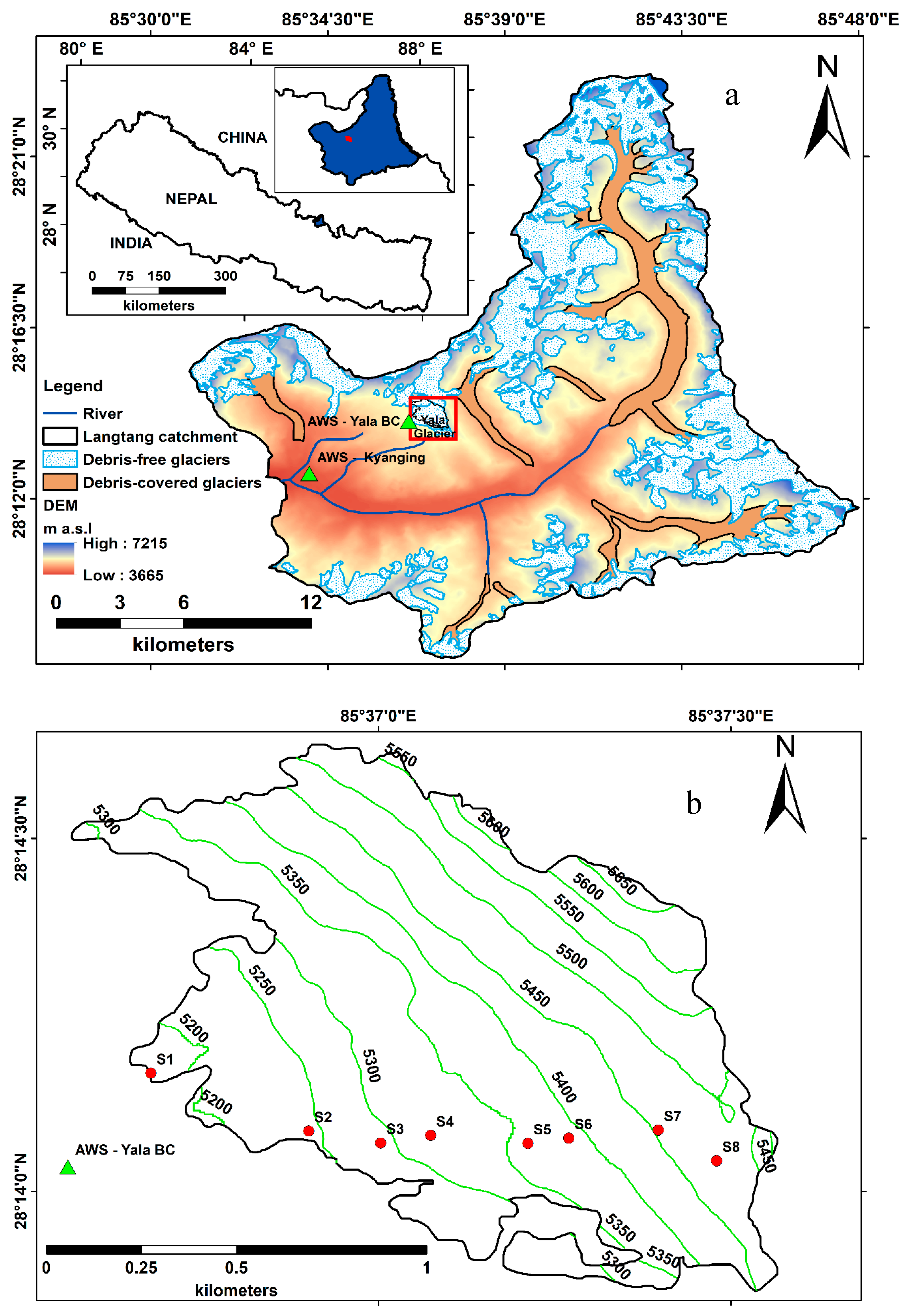
Yala Glacier (28.23526° N, 85.61263° E), a debris-free glacier lies in the Langtang River basin in Langtang Valley of Rasuwa district, Nepal. It is approximately 60 km north of Kathmandu Valley. It is a summer-accumulation type glacier and influenced by the Indian summer monsoon [19], associated with high solar radiation and high atmospheric moisture content. It covers an area of 1.37 km2 and flows from 5681 to 5143 m a.s.l. The glacier is a plateau type, it faces south-west and has an average slope of 22°. It is a benchmark glacier of the Central Himalaya [30]. Figure 1 shows the location map of the study site.
2.2. Meteorological Datasets
Meteorological data from two AWSs (AWS at Yala base camp (5060 m a.s.l.) and AWS at Kyangjing (3862 m a.s.l.)) from Campbell have been used in the model to calculate the point mass balance of the Glacier. AWS at Yala base camp was used for all calculations while AWS at Kyangjing was used to fill few missing air temperature and precipitation data at Yala base camp AWS using the temperature lapse rate of −0.0054 °C m−1 precipitation gradient of +0.041 % m−1 as determined for the Langtang valley [1]. Table 1 shows the variables measured and sensors used in the Campbell AWS and pluvio installed at Yala base camp. Measurements were taken at 10 minutes interval and averaged over one hour.
2.3. Glacier-Wide Mass Balance Using Glaciological Method
In this study, MB measurements at 8 different stakes at the elevations ranging from 5179 m a.s.l. to 5482 m a.s.l. are analyzed. Mass balance measurements on Yala Glacier have been carried out since November 2011 to present by the Cryosphere Monitoring Project (CMP). Measurements are made twice a year: in October-November and in April-May to characterize the ‘summer’ and ‘winter’ balance respectively. Various stakes installed by Chinese and Japanese researchers are also used in this study. Data from a minimum of four stakes were analyzed for 2014–2015 and a maximum of eight stakes for 2015–2016. In MB calculations, snow density was used on the basis of snow pit analysis near every stake position. Densities of snow were found to be between 200 kg m−3–532 kg m−3 during the field measurements. The density of ice was estimated to be 870 kg m−3 for Yala Glacier [30]. The length of stake above the ice and snow depth are measured at the beginning and at the end of the measurement period then multiplied with respective ice and snow densities and summed up algebraically to obtain the mass balance at every stake location (point mass balance).
The hypsometry of the Yala Glacier was obtained from ALOS PALSAR DEM (12.5 m × 12.5 m) (https://vertex.daac.asf.alaska.edu/). Glacier outline was manually delineated using a Landsat image (13 November 2017, path 141, and row 40) and verified during field visits. The annual glacier-wide mass balance (Ba) is calculated as follows:
where, bi is point mass balance at the i elevation, si is the area of elevation band i and S is the total area of the glacier.
Mass balance was obtained for discrete elevation belts with a 10 m step using linear regression between all the available observed point mass balance data and elevation. Area of every 10 m belt was multiplied by the corresponding mass balance value, summed over the entire glacier and divided by the glacier area S to obtain a glacier-wide mass balance (Ba) [38,43,44].
Equilibrium line altitude (ELA) was determined using the regression equation where the regression line crosses the zero mass balance line. Accumulation area ratio (AAR) was determined by dividing the total area where mass balance was positive by the total area of the glacier. Mass balance gradient (db/dz) was derived from the regression between the observed point mass balance and elevation.
2.4. Mass Balance Calculation using Surface Energy Balance Model
In this study, point energy and mass balance are calculated by using a mass balance model based on SEB [22]. The hourly meteorological data from AWS at Yala base camp (Table 1) along with initial surface conditions (snow density, snow depth, albedo, and roughness length) at every stake position were used to derive SEB at point scale. The same values of incoming shortwave and longwave radiation were used for all stake locations. Temperature and precipitation were calculated for each stake location using the AWS data and temperature lapse rate and precipitation gradient available from earlier studies “Section 2.2 [1]”. The model calculates ablation, using the observed hourly meteorological data. Accumulation is calculated from the solid precipitation fraction. Precipitation at the Yala Glacier occurs as solid, liquid and mixed. Correlation between air temperature and humidity is based upon the type of precipitation and this relationship is used to distinguish between snow and rain precipitation during the precipitation event [22].
The model calculates the surface temperature, which balances the right hand side of Equation (2). If surface temperature is below 0 °C, QM is taken as zero. If the surface temperature rises above 0 °C, the excess heat calculated by fixing the surface temperature at 0 °C is taken as QM. This QM is used to calculate the amount of ablation. At the end of every hour calculation, the resulting surface snow or ice temperature is used to begin the next iteration. The study was carried out for the period of 2012 (5 June–13 October), 2013 (8 May–19 November) and 2014 (5 May–15 November).
where Snet is net shortwave radiation, Lnet is net longwave radiation, is net radiation is turbulent sensible heat flux, is turbulent latent heat flux, is heat conduction flux, is energy flux from rain and is energy used to melt snow and ice in W m−2. Energy flux towards the glacier surface is taken as positive whereas energy flux away from the glacier surface is taken as negative.
In general, rainwater contributes only a very minor component of the energy balance of glaciers and hence, it is neglected during the energy balance calculations [22]. A rainfall event of 10 mm at 10 °C on a melting surface would produce a heat flux of 2.4 W m−2 averaged over a day, hence negligible compared to other heat fluxes [23].
2.4.1. Net Radiation
The incoming shortwave (Sin) and longwave (Lin) radiation fluxes were obtained from the AWS. The reflected shortwave (Sout) and outgoing longwave (Lout) radiation fluxes were calculated using albedo and emissivity values of snow and ice for each stake using Equations (3) and (4)
where, is net shortwave radiation flux and is surface albedo is the emissivity of the glacier surface which is assumed to be unity, is Stefan’s Boltzmann constant (5.67 × 10⁻⁸ W m−2 K−4), and Ts is the surface temperature (K).
Surface albedo is an important and a critical factor in the mass balance of a glacier [45,46]. In this study, snow and ice surfaces are treated individually on the basis of their different shortwave radiation absorption/reflection behavior. In this model, albedo values are iterated being within the range (0.6–0.9) for snow and (0.3–0.4) for ice on the basis of previous studies [22,47] and best albedo values, resulting in the most realistic calculations, are 0.33 for ice and 0.72 (ablation zone) and 0.81 (accumulation zone) for snow. And initial albedo values of 0.33 (ice) and 0.72 (snow) are used at every stake position in ablation zone whereas initial albedo values 0.33 for ice and 0.81 for snow are used for every stake position in accumulation zone. In the ablation zone, due to melt, there is strong temporal and spatial variation in albedo while in the accumulation zone, albedo is higher and nearly constant.
Depth of snow layer present on the glacier surface during the ablation season has an important effect on albedo, hence, relating the depth of snow to the albedo of the underlying surface [48], following equations are incorporated:
where, is the surface albedo when the thickness of snow is d in meters, is the albedo of snow, and is the albedo of the underlying surface before the snowfall that is an assumed albedo of ice. When the thickness of snow exceeds 0.02 m, the albedo of the surface is assumed to be the albedo of snow whereas, when the thickness is lower than or equal to 0.02 m then the surface albedo is calculated by model using Equation (5).
2.4.2. Turbulent Sensible Heat Flux
Turbulent sensible heat flux is the function of temperature gradient and wind speed and is given as:
where, is density of air (kg m−3), is the specific heat capacity of air at constant pressure (J kg−1 K−1), and A is the turbulent transfer coefficient, u is wind speed (m s−1), is air temperature (°C) measured at 2 m above the surface. and is surface temperature of the glacier in °C. Turbulent transfer coefficient (A) is calculated by:
where, k is the Von Karman constant 0.41, z (m) is the measurement level above the snow or ice surface, and (m) is the aerodynamic roughness length. is considered to be 0.5 × 10⁻³ m for snow and 5 × 10⁻³ m for ice [22].
2.4.3. Turbulent Latent Heat Flux
Turbulent latent heat flux, is the function of vapor pressure gradient and wind speed and calculated as:
where, L is the latent heat of evaporation (2.5 × 10⁶ J kg−1), and are the specific humidity of air at measurement level z, and specific humidity at the snow surface respectively. However, due to unavailability of , it has been calculated using the following equation based on the values of atmospheric pressure (), vapor pressure of the air () and saturation vapor pressure at the snow surface ( ) (all in 103 Pa).
Substituting the value of in Equation (9), the Equation (8) for becomes
where, (Pa) is calculated from the saturation vapor pressure over a plane surface of the pure water using the Goff–Gratch formulation and the prevailing relative humidity. (Pa) is assumed to be the same as the saturation vapor pressure over a plane surface of pure water at surface temperature Ts.
2.4.4. Heat Conduction Flux
Heat conduction into the glacier from the surface is calculated using Equation (11) where no meltwater percolation is assumed [22].
where, is the thermal conductivity of snow (W m−1 K−1), and is the temperature gradient. Temperature profile between the surface and a depth of 10.24 m with a step of 0.02 m was calculated with the following thermodynamic equation.
where is the density of snow or ice (kg m−3), is the specific heat capacity of ice (2009 J kg−1 K−1) and, t is time.
Thermal conductivity is obtained using the following equation [49]:
2.4.5. Point Mass Balance
The algebraic sum of the individual SEB components and solid precipitation (Ps) gives the point mass balance of a glacier as follows:
where is latent heat of fusion (3.34 × 10⁵ J Kg−1). Point mass balance represents mass balance at stake location. The glacier-wide mass balance is calculated using Equation (1).
3. Results
3.1. Meteorological Conditions at the Study Site
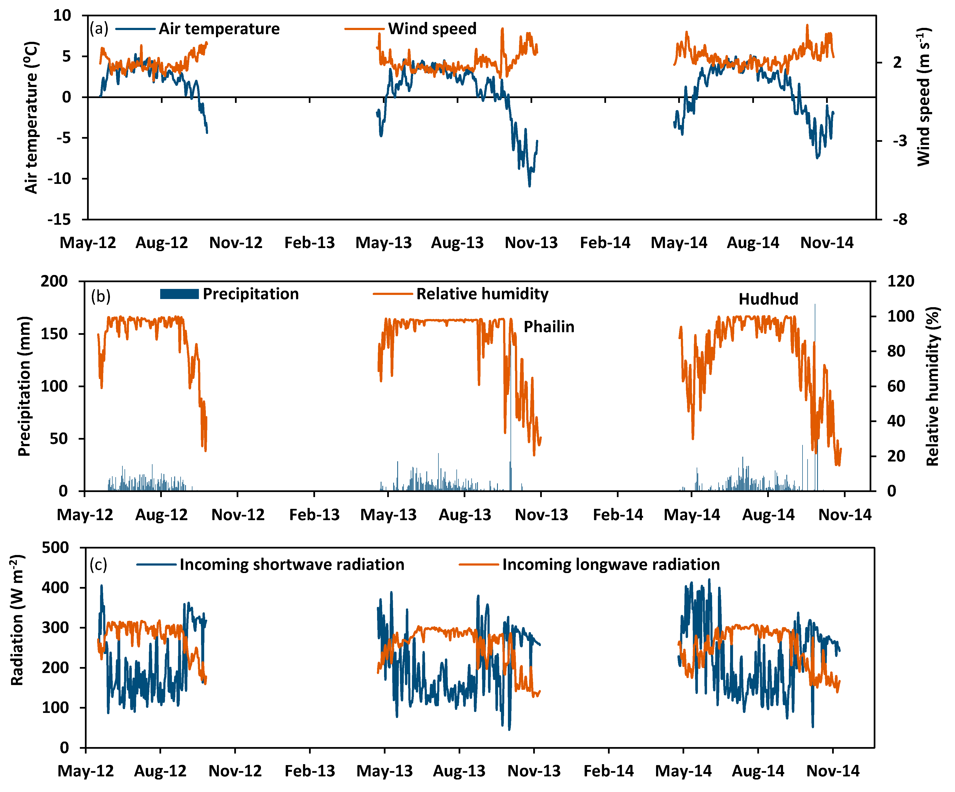
Figure 2 shows the daily mean values of air temperature, wind speed, relative humidity (RH), precipitation, incoming longwave radiation and incoming shortwave radiation recorded at Yala base camp AWS at 5060 m a.s.l. for the period of 2012 (5 June–13 October), 2013 (8 May–15 November) and 2014 (5 May–19 November).
Daily air temperature ranges between 5.3 °C and −10.9 °C for the considered periods. From June to September (monsoon season) daily mean temperature rose above 0 °C. Similarly, RH changed markedly, however, during monsoon period RH values were very high (>90 %) because of frequent precipitation events. On an average, 78% of the total precipitation falls during the monsoon. Cyclones, Phailin (13–15 October 2013) and Hudhud (15 October 2014) events brought the extremely large amount of precipitation 194 mm and 179 mm respectively within a few days. Such events are extreme and, if they are not considered, precipitation during the monsoon season accounts for 89% of precipitation recorded during the study period. Wind speed is low and never exceeded 3.1 m s−1 for the monsoon period whereas high value of 4.4 m s−1 is observed during 14 October 2014. Incoming shortwave radiation is maximum during May with an average value of 284 W m−2. Conversely, incoming longwave radiation is very high during monsoon with an average value of 280 W m−2.
3.2. Observed Mass Balance
3.2.1. Annual and Cumulative Glacier-Wide Mass Balance of Yala Glacier
Table 2 shows the annual glacier wide mass balances (Ba), seasonal glacier wide mass balances, ELA, AAR and mass balance gradients of Yala Glacier for the period of November 2011–November 2017. Annual mass balance values were negative during the entire study period with high negative values observed in 2016–17 particularly in comparison with 2012–13 and 2013–14 mass balance years. Cumulative mass balance was −4.88 m w.e., mean annual glacier-wide mass balance (Ba) of −0.81 m w.e. a−1 with mean annual variability of ±0.48 (standard deviation) were observed for the duration of 2011–17. The mean annual ELA was 5457 m a.s.l with mean AAR and steep mass balance gradient of 0.28 and 1.08 m w.e. (100 m)−1 a−1 respectively. ELA is increasing for every year except for 2012–2013 and 2013–2014. AAR decreased strongly after 2015. Very high ELA value of 5555 m a.s.l. and very low AAR value of 0.06 were observed in 2016–2017.
Both positive and negative components of mass balance are a function of density of snow and ice, and depth of snow layer. Accuracy of the overall glacier wide annual mass balance is determined and presented on the basis of errors in stake reading, errors in ice/snow density measurements, errors in snow depth measurements, errors in the representatives of stakes or accumulation measurement sites (sampling error) and the period of study considered [50]. In this study, errors in the positive and negative mass balances are determined to be ±0.15 m w.e. a−1 and ±0.19 m w.e. a−1 respectively while sampling error is found to be ±0.12 m w.e. a−1, which results in the error of ±0.27 m w.e. a−1.
The annual mass balance gradients of Yala Glacier are shown in Figure S1 for the measuring period of November 2011–November 2017. The regression lines are plotted over annual point MBs measured in the debris-free Yala Glacier between 5143 and 5681 m a.s.l. A steep mean mass balance gradient (1.08 m w.e. (100)−1 a−1) is observed for the Yala Glacier (Table 2). Mass balance gradients of Nepalese glaciers can differ in between 0.5 m w.e. (100 m−1) to 1.5 m w.e. (100 m−1) depending on the size and aspect of the glacier [38]. The obtained mass balance gradient values ranging from 0.86 m w.e. (100)−1 to 1.4 m w.e. (100)−1 for the Yala Glacier are within the range of the published values and are comparable to those observed in the Alps, Western Himalaya or mid-latitude glaciers [38,51]. Few snow and glacier melt models at watershed scale in the Himalayan region are developed based on ablation gradient only [52]. These models can therefore be improved in the future using different MB gradients for different glacier zones depending on debris-covered or its ablation and accumulation areas.
3.2.2. Seasonal Glacier-wide Mass Balance
Winter and summer glacier-wide mass balances (Table 2) are derived on the basis of glaciological field measurements conducted twice in a year. More negative summer balance with the value of −1.97 m w.e. is observed for the period of 2016–2017 and less negative summer value of −0.32 m w.e. is observed for the period of 2012–2013. More negative mass balance, indicating more ablation during summer is observed for all the considered years despite of being summer-accumulation type glacier [19,36]. Every winter experiences positive mass balance and do not vary strongly except for the period of the mass balance year 2012–2013 and never exceeded more than +0.24 m w.e. throughout the study period. This indicates that the winter can experience accumulation, which is very limited.
3.3. Calculated (Modelled) Energy and Mass Balance
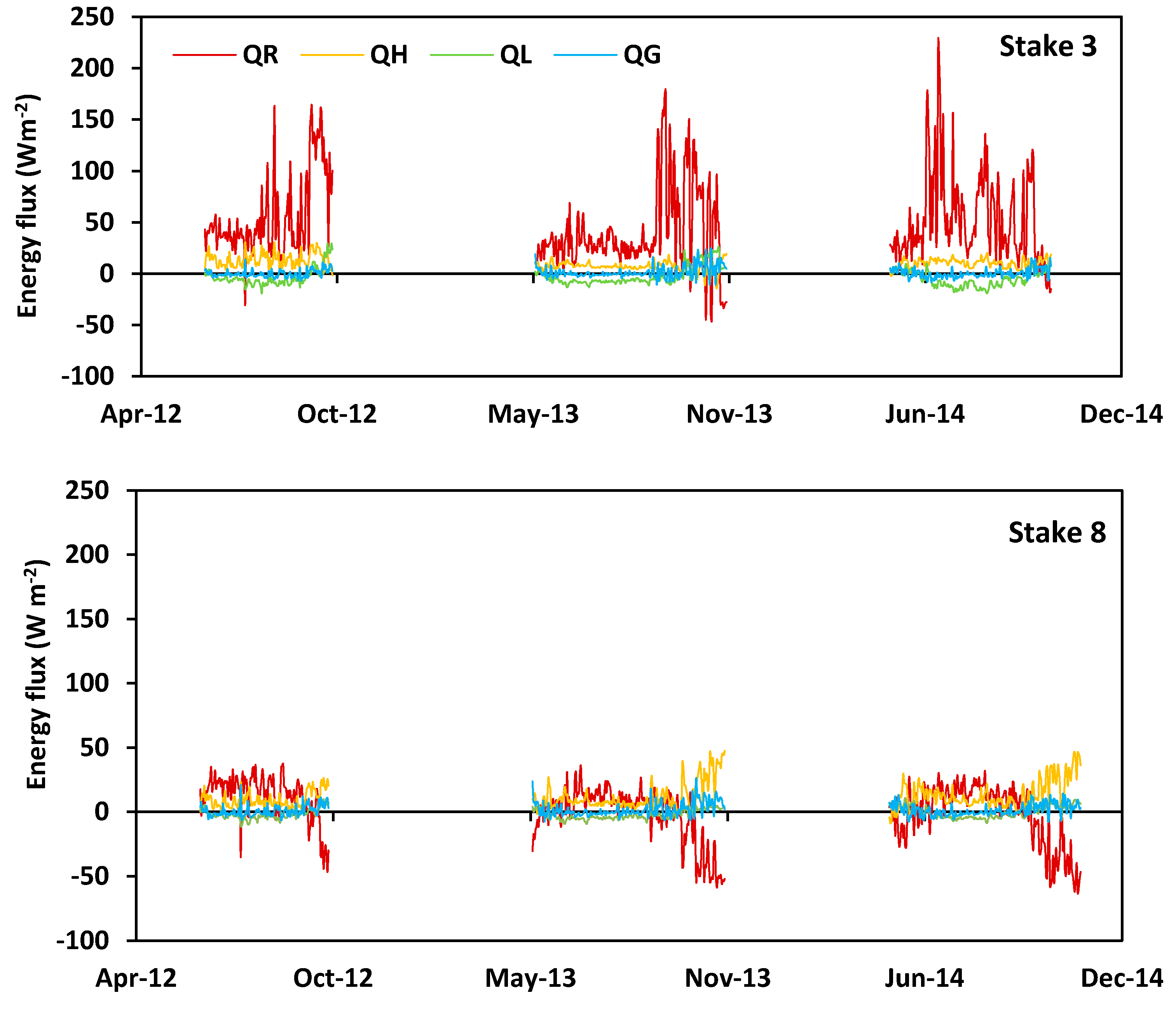
Calculated daily mean values and percentage of surface energy balance components at different stake locations on the Yala Glacier during the summer of 2012, 2013, and 2014 are shown in Figure 3 and Table 3. The contribution of net radiation flux to glacier surface melting is high in comparison to the rest of the components (sensible, latent, and heat conduction). Positive turbulent sensible heat flux indicates heat transfers to the glacier surface throughout the melting season. The turbulent latent heat is usually negative which implies that the evaporation exceeded condensation because of high temperature and low precipitation. The contribution of net radiation flux is very high at lower elevations (below 5451 m a.s.l.) in all three years (Table S1). There is a high variation of net radiation in the ablation and accumulation area of the glacier. It is because of the different albedo and snow depths in higher altitudes. Snow depth and albedo are higher in both stake 7 and stake 8 than at the lower stakes. As more snow with high albedo was present in the accumulation area (stakes 7 and 8), value of net radiation was low in 2012 (Table S1) and net radiation contributed very little to melt in 2013 and 2014. Moreover, extreme precipitation, brought by the cyclones Phailin and Hudhud which hit the area in October 2013 and October 2014, respectively, maintained the high albedo of snow in the accumulation area in the post-monsoon season. Therefore, melt was weak sustained by QH and QG. Similar conditions were observed in 2013 and 2014. Sensible heat contributes significantly to melt particularly at the end of summer season (Figure 3). This is because surface temperature decreases strongly in comparison with air temperature. The contribution of the conduction heat flux is relatively small but increases at higher elevations (Figure 3, stake 8).
3.4. Glacier-Wide Mass Balance
Table 4 shows the modelled summer mass balance in 2012, 2013, and 2014 and observed summer mass balance of Yala Glacier in 2013 and 2014. The modelled and observed results show more negative mass balance for all considered summer period, indicating more ablation than accumulation. Equilibrium line altitude (ELA) are also calculated and agree well with the observed ELA values. The magnitude of errors in mass balances for the summer 2013 and 2014 are 3.1% and 3.8% respectively, whereas magnitude of errors in ELA determination are 0.02% and 0.04% for the summer 2013 and 2014 respectively.
3.5. Validation of Energy-Mass Balance Model
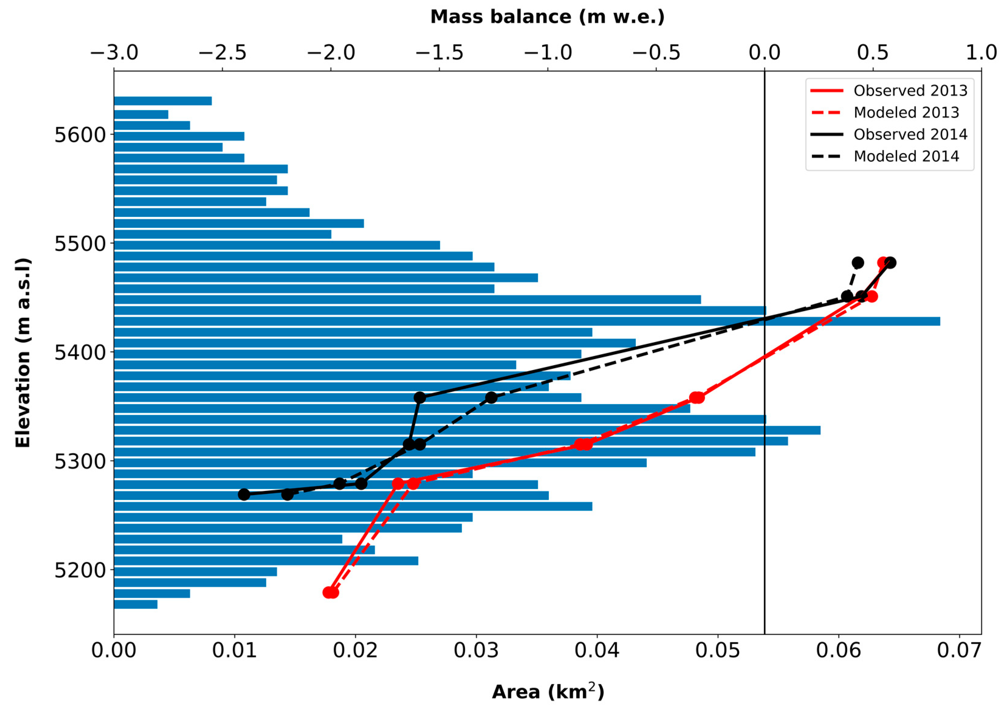
The modelled point mass balance is compared with the observed point mass balance of the Yala Glacier for two consecutive summer seasons of 2013 and 2014 as shown in Table 5. Figure 4 displays the difference between modelled and observed summer mass balance values. At every stake location, the observed and modelled values are in good agreement although discrepancies increase at higher elevations (stakes 5, 7 and 8).
3.6. Sensitivity Analysis
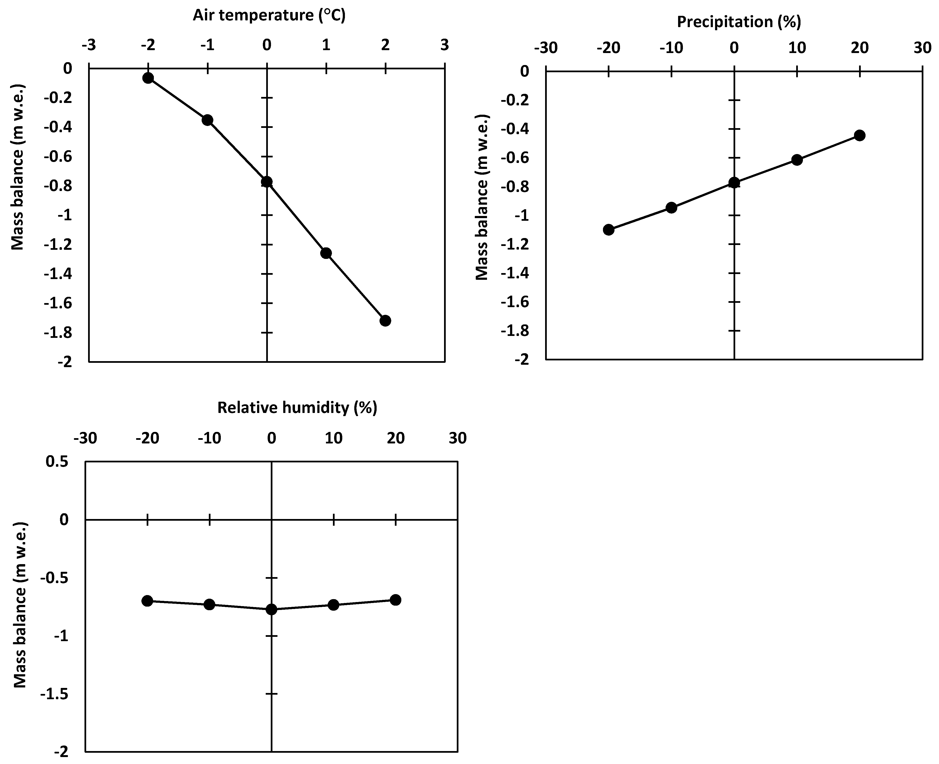
Sensitivity of mass balance to changes in air temperature, precipitation, and relative humidity were conducted using data from 2014 (Figure 5). Air temperature was altered by ±1 °C and ±2 °C whereas relative humidity and precipitation were altered by ±10 % and ±20 %. When temperature is increased by 1 °C, the value of mass balance becomes −1.26 m w.e. from the reference case of −0.77 m w.e. whereas it moves towards less negative side (−0.35 m w.e.) when the air temperature is decreased by 1 °C. Subsequently same increasing and decreasing pattern is seen when it is increased and decreased by 2 °C (−1.72 m w.e. and −0.066 m w.e.). Reduction/increase in precipitation results in the enhancement/impediment of net negative mass balance. With an increment of precipitation by 10% and 20% displays the less negative mass balance values of −0.62 m w.e. and −0.45 m w.e. respectively, whereas, with a decrement of precipitation by 10% and 20% shows the more negative mass balance values of −0.95 m w.e. and −1.1 m w.e. respectively. Mass balance is found to be less sensitive to relative humidity in comparison to other variables. With increment in relative humidity by 10% and 20%, net mass balance shows very small change, −0.69 m w.e. being the highly altered value when relative humidity is increased by 20%.
Sensitivity analysis is also performed for the initial surface parameters altering values in snow density, ice density, snow albedo, ice albedo, and roughness length as shown in Table 6. The mass balance is most sensitive to the albedo of snow and least sensitive to the roughness length as only 3.7% difference is seen even though roughness length is increased by 25%. When albedo of snow is increased by 0.1, mass balance value changes by 18% in comparison with its reference value. This is because the surface albedo has a strong effect on net radiation, which is the most important contributor to the melting. Density and roughness length do not affect the mass balance appreciably because their effect appears only in the heat conduction, and sensible and latent heat fluxes, respectively. These heat fluxes make relatively small contributions to the total energy available for melting, compared with the net radiation.
4. Discussion
4.1. Annual and Seasonal Glacier-Wide Mass Balance
Annual Ba, ELA, AAR, and mass balance gradients for Yala glacier have been observed for the period of 2011 to 2017. In this study period Yala Glacier is found to be losing its mass at an accelerated rate with an average annual MB rate of −0.81 ± 0.27 m w.e. a−1. The highest negative value of MB (−1.73 m w.e.) is observed for the period of 2016–2017 and the lowest negative MB value (−0.31 m w.e.) is observed for the period of 2012–2013. Low air temperature of 0.34 ℃ compared to other years in the summer of 2013 promoted the less negative mass balance value in 2013 (Table S1). Moreover, bountiful precipitation of 1057 mm including cyclone Phailin during the end of summer 2013 also contributed for this result. As, summer is the major season responsible for the melting and hence, determining the MB of a glacier [19]. Even though, precipitation is higher in the summer of 2014, the mean observed air temperature is quite high, more than double of the mean value observed in the summer of 2013 (Table S1). So, this resulted into the more negative MB value in 2013–2014, as MB is more sensitive to air temperature than the precipitation.
4.2. Comparison of Present Mass Balance and Energy Balance Studies with Other Studies in the High Mountain Asia
Present study shows the similar result to the previous studies in the High Mountain Asia, i.e., negative mass balances. MB of Yala Glacier was estimated to be −0.89 m w.e. for the period of November 2011–November 2012 [37]. Small glaciers such as Pokalde (0.1 km2) and West Changri Nup (0.92 km2) had mean MBs of −0.69 ± 0.28 m w.e. a−1 and −1.24 ± 0.27 m w.e. a−1 for the period of 2009–15 and 2010–15 respectively [16], and from this study mean MB of the Yala Glacier was observed as −0.81 ± 0.27 m w.e. a−1 which lies between MBs of West Changri Nup and Pokalde glaciers. However, Mera Glacier (5.1 km2), located at higher elevations, had mass balance of −0.03 ± 0.28 m w.e. a−1 which indicated almost balanced conditions, it might be because the more area of the glacier is located at highest elevations. Indeed, low maximum-elevation glaciers, such as Pokalde, Changri Nup and Yala experience ablation over the entire surface area with low-albedo bare ice exposed to their highest elevations and the accumulation zone reduced very significantly (Table 2).
Analysis of relative contributions of the components of energy balance to melt were conducted at several other Himalayan glaciers. It has been concluded that the net radiation is the dominant energy factor for the melting of Himalayan glaciers. This is because of high incoming shortwave radiation during the clear sky condition in the summer. The net longwave radiation is mostly negative with its high value during the peak monsoon due to warm, humid and cloudy atmosphere. Contribution of net radiation in Yala Glacier ranges from 66% to 61% for the stake positions up to 5358 m a.s.l. Study conducted in 25 May–25 Sep 1978 on Glacier AX010 in the Central Himalaya showed 85% contribution of the net radiation followed by sensible heat flux (10%) and latent heat flux (5%) at an elevation of 4960 m a.s.l. [22]. Similarly, study carried out in 8 Jul–5 Sep 2013 on Chhota Shigri Glacier in western Himalaya also revealed the 80% contribution [53] of net radiation whereas sensible and latent heat fluxes contributions were found to be 13% and 5% respectively at an elevation of 4670 m a.s.l. A study conducted in the Glacier Parlung No. 4 in Southeast Tibetan Plateau during 21 May–8 Sep 2009 resulted in the 86% contribution of net radiation followed by sensible (16%) and latent (−1%) fluxes at an elevation of 4800 m a.s.l. [54]. For the observation period of 4 Oct 2009–15 Sept 2011 in Zhadang Glacier [29], the radiation component contributed 82% of the total energy fluxes. This was followed by 10% and 6% contributions of sensible and latent heat fluxes respectively. The published results agree well with those obtained for the Yala Glacier. However, the results signify that the net radiation contribution decreases for the increasing altitude. Moreover, Yala Glacier is not surrounded by mountain walls, it is a plateau type glacier so, incoming longwave radiation is reduced and hence, lesser value of net radiation is observed. Sensible heat flux is positive on the Yala Glacier during the summer which means heat is transported to the glacier surface. The values of sensible heat flux are higher during the post-monsoon season than during the monsoon. This can be due to the clear sky condition during October and November which enhances the high temperature gradient. Moreover, wind speeds are also high in these months. Positive heat conduction is calculated for this study on the Yala Glacier. Heat conduction flux represented a very minor proportion (2%) of the total heat flux on Zhadang Glacier for two years of observation period [29]. Similarly, heat conduction flux on Chhota Shigri Glacier in Western Himalaya was also estimated to be 2% for the summer [28]. On the other hand, in the ablation zone of Parlung No. 4 Glacier in southeast Tibetan Plateau, negative heat conduction flux was observed (−1%) [54]. Similar contribution pattern of 0.10% and 0.56% are seen at the lower altitudes of the Yala Glacier.
5. Conclusions
This study presented results of analysis of a six-year dataset of annual and seasonal mass balance values measured using the direct glaciological method between November 2011 and November 2017. It also presents the use of energy balance model to predict the summer mass and energy balance for the period of 2011–2014 for Yala Glacier. Yala Glacier has been losing its mass rapidly with the mean annual mass balance of −0.81 ± 0.27 m w.e. a−1 (2011–2017). While comparing with other glaciers, small and low altitude glaciers like Yala in the Himalaya are losing their mass at accelerated rate.
Energy balance study shows that the net radiation flux is the primary energy source for the melting of glacier ice and snow. Sensible heat flux and heat conduction are the secondary components responsible for the melting. The net shortwave radiation contribution is very high in lower part of the glacier compared to the upper part because of higher albedo values in the upper part. Sensitivity analysis of mass balance to the input meteorological and surface parameters showed that the mass balance is highly sensitive to the change in air temperature, precipitation, and albedo of the snow. Mass balance was found to be considerably less sensitive to changes in relative humidity and moderately sensitive to changes in snow density.
Supplementary Materials
The following are available online at https://www.mdpi.com/2073-4441/11/1/6/s1, Figure S1: Annual mass balance (dots) of Yala Glacier from 2011 to 2017 as a function of altitude derived from the field measurements, Table S1: Total contribution of energy balance components to the surface melting at various stake locations on Yala Glacier for the period of 5 June 2012–13 October 2012 (131 days), 8 May 2013–19 November 2013 (195 days) and 5 May 2014–15 November 2014 (196 days), Table S2: Mean meteorological variables measured at Yala base camp AWS (5060 m a.s.l.) on Yala Glacier for the period June 2012–October 2012, May 2013–November 2013 and May 2014–November 2014.
Author Contributions
A.A. conducted this research work and finalized the manuscript. The Project leadership was assumed by R.B.K. who also analyzed the initial draft. He also discussed the results with me and contributed to the preparation of final manuscript.
Funding
The Hindu Kush Himalaya (HKH) Cryosphere Monitoring Project implemented by International Centre for Integrated Mountain Development (ICIMOD) and supported by the Norwegian Ministry of Foreign Affairs.
Acknowledgments
We would like to thank the HKH Cryosphere Monitoring Project implemented by International Centre for Integrated Mountain Development (ICIMOD) and supported by the Norwegian Ministry of Foreign Affairs. We would also like to thank project partners for their help in carrying out this study including The Himalayan Cryosphere, Climate and Disaster, Research Center, Kathmandu University, Central Department of Hydrology and Meteorology, Tribhuwan University, Department of Hydrology and Meteorology, Government of Nepal and Water and Energy Commission Secretariat, Government of Nepal. We are also thankful to Rakesh Kayastha, Ravi Raj Shrestha, Tika Ram Gurung, Gunjan Silwal and Sunwi Maskey for their valuable suggestions while carrying out this study.
Conflicts of Interest
We have no conflict of interests.
References
- Immerzeel, W.W.; Petersen, L.; Ragettli, S.; Pellicciotti, F. The Importance of Observed Gradients of Air Temperature and Precipitation for Modeling Runoff from a Glacierized Watershed in the Nepalese Himalayas. Water Resour. Res. 2014, 50, 2212–2226. [Google Scholar] [CrossRef]
- Immerzeel, W.W.; Pellicciotti, F.; Bierkens, M.F.P. Rising River Flows throughout the Twenty-First Century in Two Himalayan Glacierized Watersheds. Nat. Geosci. 2013, 6, 742–745. [Google Scholar] [CrossRef]
- Immerzeel, W.W.; Van Beek, L.P.; Bierkens, M.F. Climate Change Will Affect the Asian Water Towers. Science 2010, 328, 1382–1385. [Google Scholar] [CrossRef] [PubMed]
- Kaser, G.; Cogley, J.G.; Dyurgerov, M.B.; Meier, M.F.; Ohmura, A. Mass Balance of Glaciers and Ice Caps: Consensus Estimates for 1961–2004. Geophys. Res. Lett. 2006, 33. [Google Scholar] [CrossRef]
- Bolch, T.; Kulkarni, A.; Kääb, A.; Huggel, C.; Paul, F.; Cogley, J.G.; Frey, H.; Kargel, J.S.; Fujita, K.; Scheel, M. The State and Fate of Himalayan Glaciers. Science 2012, 336, 310–314. [Google Scholar] [CrossRef] [PubMed] [Green Version]
- Bahadur, J. The Himalayas: A Third Polar Region. In Snow and Glacier Hydrology, Proceedings of the International Symposium, Kathmandu, Nepal, 16–21 November 1992; IAHS Publication: Wallingford, UK, 1993; Volume 218, pp. 181–190. [Google Scholar]
- Wang, X.; Tseng, Z.J.; Li, Q.; Takeuchi, G.T.; Xie, G. From “third Pole”to North Pole: A Himalayan Origin for the Arctic Fox. Proc. R. Soc. B 2014, 281, 20140893. [Google Scholar] [CrossRef]
- Yao, T.; Thompson, L.; Yang, W.; Yu, W.; Gao, Y.; Guo, X.; Yang, X.; Duan, K.; Zhao, H.; Xu, B. Different Glacier Status with Atmospheric Circulations in Tibetan Plateau and Surroundings. Nat. Clim. Chang. 2012, 2, 663–667. [Google Scholar] [CrossRef]
- De Smedt, B.; Pattyn, F. Numerical Modelling of Historical Front Variations and Dynamic Response of Sofiyskiy Glacier, Altai Mountains, Russia. Ann. Glaciol. 2003, 37, 143–149. [Google Scholar] [CrossRef]
- Oerlemans, J. Quantifying Global Warming from the Retreat of Glaciers. Science 1994, 264, 243–245. [Google Scholar] [CrossRef] [Green Version]
- Oerlemans, J. Glaciers as Indicators of a Carbon Dioxide Warming. Nature 1986, 320, 607–609. [Google Scholar] [CrossRef]
- Vincent, C.; Ribstein, P.; Favier, V.; Wagnon, P.; Francou, B.; Le Meur, E.; Six, D. Glacier Fluctuations in the Alps and in the Tropical Andes. C. R. Geosci. 2005, 337, 97–106. [Google Scholar] [CrossRef]
- Bolch, T.; Pieczonka, T.; Benn, D.I. Multi-Decadal Mass Loss of Glaciers in the Everest Area (Nepal Himalaya) Derived from Stereo Imagery. Cryosphere 2011, 5, 349–358. [Google Scholar] [CrossRef]
- Mayewski, P.A.; Jeschke, P.A. Himalayan and Trans-Himalayan Glacier Fluctuations since AD 1812. Arct. Alp. Res. 1979, 11, 267–287. [Google Scholar] [CrossRef]
- Bajracharya, S.R.; Maharjan, S.B.; Shrestha, F.; Guo, W.; Liu, S.; Immerzeel, W.; Shrestha, B. The Glaciers of the Hindu Kush Himalayas: Current Status and Observed Changes from the 1980s to 2010. Int. J. Water Resour. Dev. 2015, 31, 161–173. [Google Scholar] [CrossRef]
- Sherpa, S.F.; Wagnon, P.; Brun, F.; Berthier, E.; Vincent, C.; Lejeune, Y.; Arnaud, Y.; Kayastha, R.B.; Sinisalo, A. Contrasted Surface Mass Balances of Debris-Free Glaciers Observed between the Southern and the Inner Parts of the Everest Region (2007–2015). J. Glaciol. 2017, 63, 637–651. [Google Scholar] [CrossRef]
- Gardelle, J.; Berthier, E.; Arnaud, Y. Slight Mass Gain of Karakoram Glaciers in the Early Twenty-First Century. Nat. Geosci. 2012, 5, 322–325. [Google Scholar] [CrossRef]
- Hewitt, K. The Karakoram Anomaly? Glacier Expansion and the “elevation effect,” Karakoram Himalaya. Mt. Res. Dev. 2005, 25, 332–340. [Google Scholar] [CrossRef]
- Ageta, Y.; Higuchi, K. Estimation of Mass Balance Components of a Summer-Accumulation Type Glacier in the Nepal Himalaya. Geogr. Ann. Ser. Phys. Geogr. 1984, 66, 249–255. [Google Scholar] [CrossRef]
- Quincey, D.J.; Braun, M.; Glasser, N.F.; Bishop, M.P.; Hewitt, K.; Luckman, A. Karakoram Glacier Surge Dynamics. Geophys. Res. Lett. 2011, 38. [Google Scholar] [CrossRef]
- Fujita, K.; Ageta, Y. Effect of Summer Accumulation on Glacier Mass Balance on the Tibetan Plateau Revealed by Mass-Balance Model. J. Glaciol. 2000, 46, 244–252. [Google Scholar] [CrossRef]
- Kayastha, R.B.; Ohata, T.; Ageta, Y. Application of a Mass-Balance Model to a Himalayan Glacier. J. Glaciol. 1999, 45, 559–567. [Google Scholar] [CrossRef]
- Hock, R. Glacier Melt: A Review of Processes and Their Modelling. Prog. Phys. Geogr. 2005, 29, 362–391. [Google Scholar] [CrossRef]
- Hock, R. Temperature Index Melt Modelling in Mountain Areas. J. Hydrol. 2003, 282, 104–115. [Google Scholar] [CrossRef]
- Hock, R. A Distributed Temperature-Index Ice-and Snowmelt Model Including Potential Direct Solar Radiation. J. Glaciol. 1999, 45, 101–111. [Google Scholar] [CrossRef]
- Laumann, T.; Reeh, N. Sensitivity to Climate Change of the Mass Balance of Glaciers in Southern Norway. J. Glaciol. 1993, 39, 656–665. [Google Scholar] [CrossRef]
- Oerlemans, J.; Anderson, B.; Hubbard, A.; Huybrechts, P.; Johannesson, T.; Knap, W.H.; Schmeits, M.; Stroeven, A.P.; Van de Wal, R.S.W.; Wallinga, J. Modelling the Response of Glaciers to Climate Warming. Clim. Dyn. 1998, 14, 267–274. [Google Scholar] [CrossRef]
- Nemec, J.; Huybrechts, P.; Rybak, O.; Oerlemans, J. Reconstruction of the Annual Balance of Vadret Da Morteratsch, Switzerland, since 1865. Ann. Glaciol. 2009, 50, 126–134. [Google Scholar] [CrossRef]
- Zhang, G.; Kang, S.; Fujita, K.; Huintjes, E.; Xu, J.; Yamazaki, T.; Haginoya, S.; Wei, Y.; Scherer, D.; Schneider, C. Energy and Mass Balance of Zhadang Glacier Surface, Central Tibetan Plateau. J. Glaciol. 2013, 59, 137–148. [Google Scholar] [CrossRef]
- Fijita, K.; Takeuchi, N.; Seko, K. Glaciological observations of Yala Glacier in Langtang Valley, Nepal Himalayas, 1994 and 1996. Bull. Glacier Res. 1998, 16, 75–78. [Google Scholar]
- Nuimura, T.; Fujita, K.; Yamaguchi, S.; Sharma, R.R. Elevation Changes of Glaciers Revealed by Multitemporal Digital Elevation Models Calibrated by GPS Survey in the Khumbu Region, Nepal Himalaya, 1992–2008. J. Glaciol. 2012, 58, 648–656. [Google Scholar] [CrossRef]
- Fujii, Y. Field Experiment on Glacier Ablation under a Layer of Debris Cover. J. Jpn. Soc. Snow Ice 1977, 39, 20–21. [Google Scholar] [CrossRef] [Green Version]
- Fujita, K.; Nakawo, M.; Fujii, Y.; Paudyal, P. Changes in Glaciers in Hidden Valley, Mukut Himal, Nepal Himalayas, from 1974 to 1994. J. Glaciol. 1997, 43, 583–588. [Google Scholar] [CrossRef]
- Ageta, Y.; Naito, N.; Nakawo, M.; Fujita, K.; Shankar, K.; Pokhrel, A.P.; Wangda, D. Study Project on the Recent Rapid Shrinkage of Summer-Accumulation Type Glaciers in the Himalayas. Bull. Glaciol. Res. 2001, 18, 45–49. [Google Scholar]
- Fujita, K.; Kadota, T.; Rana, B.; Kayastha, R.B.; Ageta, Y. Shrinkage of Glacier AX010 in Shorong Region, Nepal Himalayas in the 1990s. Bull. Glaciol. Res. 2001, 18, 51–54. [Google Scholar]
- Ageta, Y.; Ohata, T.; Tanaka, Y.; Ikegami, K.; Higuchi, K. Mass Balance of Glacier AX010 in Shorong Himal, East Nepal during the Summer Monsoon Season. J. Jpn. Soc. Snow Ice 1980, 41, 34–41. [Google Scholar] [CrossRef]
- Baral, P.; Kayastha, R.B.; Immerzeel, W.W.; Pradhananga, N.S.; Bhattarai, B.C.; Shahi, S.; Galos, S.; Springer, C.; Joshi, S.P.; Mool, P.K. Preliminary Results of Mass-Balance Observations of Yala Glacier and Analysis of Temperature and Precipitation Gradients in Langtang Valley, Nepal. Ann. Glaciol. 2014, 55, 9–14. [Google Scholar] [CrossRef]
- Wagnon, P.; Vincent, C.; Arnaud, Y.; Berthier, E.; Vuillermoz, E.; Gruber, S.; Ménégoz, M.; Gilbert, A.; Dumont, M.; Shea, J.M. Seasonal and Annual Mass Balances of Mera and Pokalde Glaciers (Nepal Himalaya) since 2007. Cryosphere 2013, 7, 1769–1786. [Google Scholar] [CrossRef]
- Pellicciotti, F.; Stephan, C.; Miles, E.; Herreid, S.; Immerzeel, W.W.; Bolch, T. Mass-Balance Changes of the Debris-Covered Glaciers in the Langtang Himal, Nepal, from 1974 to 1999. J. Glaciol. 2015, 61, 373–386. [Google Scholar] [CrossRef]
- Naito, N.; Kadota, T.; Fujita, K.; Sakai, A.; Nakawo, M. Surface Lowering over the Ablation Area of Lirung Glacier, Nepal Himalayas. Bull. Glaciol. Res. 2002, 19, 41–46. [Google Scholar]
- Chand, M.B.; Kayastha, R.B.; Parajuli, A.; Mool, P.K. Seasonal Variation of Ice Melting on Varying Layers of Debris of Lirung Glacier, Langtang Valley, Nepal. Proc. Int. Assoc. Hydrol. Sci. 2015, 368, 21–26. [Google Scholar] [CrossRef]
- Cogley, J.G. Geodetic and Direct Mass-Balance Measurements: Comparison and Joint Analysis. Ann. Glaciol. 2009, 50, 96–100. [Google Scholar] [CrossRef]
- Wagnon, P.; Linda, A.; Arnaud, Y.; Kumar, R.; Sharma, P.; Vincent, C.; Pottakkal, J.G.; Berthier, E.; Ramanathan, A.; Hasnain, S.I.; et al. Four Years of Mass Balance on Chhota Shigri Glacier, Himachal Pradesh, India, a New Benchmark Glacier in the Western Himalaya. J. Glaciol. 2007, 53, 603–611. [Google Scholar] [CrossRef]
- Fountain, A.G.; Vecchia, A. How Many Stakes Are Required to Measure the Mass Balance of a Glacier? Geogr. Ann. Ser. Phys. Geogr. 1999, 81, 563–573. [Google Scholar] [CrossRef]
- Fujita, K. Effect of Dust Event Timing on Glacier Runoff: Sensitivity Analysis for a Tibetan Glacier. Hydrol. Process. 2007, 21, 2892–2896. [Google Scholar] [CrossRef]
- Van de Wal, R.S.W.; Oerlemans, J.; Van der Hage, J.C. A Study of Ablation Variations on the Tongue of Hintereisferner, Austrian Alps. J. Glaciol. 1992, 38, 319–324. [Google Scholar] [CrossRef]
- Cuffey, K.M.; Paterson, W.S.B. Mass Balance Processes: 2. Surface Ablation and Energy Budget. In The Physics of Glaciers, 4th ed.; Butterworth-Heinemann of Elsevier: Oxford, UK, 2010; pp. 137–173. ISBN 978-0-12-369461-4. [Google Scholar]
- Ohata, T.; Ikegami, K.; Higuchi, K. Albedo of Glacier AX 010 during the Summer Season in Shorong Himal, East Nepal. J. Jpn. Soc. Snow Ice 1980, 41, 48–54. [Google Scholar] [CrossRef]
- Van Dusen, M.S. Thermal Conductivity of Non-Metallic Solids. Int. Crit. Tables Numer. Data Phys. Chem. Technol. 1929, 5, 216–217. [Google Scholar]
- Thibert, E.; Blanc, R.; Vincent, C.; Eckert, N. Glaciological and Volumetric Mass-Balance Measurements: Error Analysis over 51 Years for Glacier de Sarennes, French Alps. J. Glaciol. 2008, 54, 522–532. [Google Scholar] [CrossRef]
- Zemp, M.; Hoelzle, M.; Haeberli, W. Six Decades of Glacier Mass-Balance Observations: A Review of the Worldwide Monitoring Network. Ann. Glaciol. 2009, 50, 101–111. [Google Scholar] [CrossRef]
- Racoviteanu, A.E.; Armstrong, R.; Williams, M.W. Evaluation of an Ice Ablation Model to Estimate the Contribution of Melting Glacier Ice to Annual Discharge in the Nepal Himalaya. Water Resour. Res. 2013, 49, 5117–5133. [Google Scholar] [CrossRef]
- Azam, M.F.; Wagnon, P.; Vincent, C.; Ramanathan, A.L.; Favier, V.; Mandal, A.; Pottakkal, J.G. Processes Governing the Mass Balance of Chhota Shigri Glacier (Western Himalaya, India) Assessed by Point-Scale Surface Energy Balance Measurements. Cryosphere 2014, 8, 2195–2217. [Google Scholar] [CrossRef]
- Yang, W.; Guo, X.; Yao, T.; Yang, K.; Zhao, L.; Li, S.; Zhu, M. Summertime Surface Energy Budget and Ablation Modeling in the Ablation Zone of a Maritime Tibetan Glacier. J. Geophys. Res. Atmos. 2011, 116. [Google Scholar] [CrossRef]
Figure 1.
(a) Map of Langtang catchment (blue polygon) in the inset map of Nepal. Location of Yala Glacier (inside the red box), Kyangjing and Yala base camp (BC) Automatic Weather Stations (AWSs) (green triangles) in Langtang catchment. (b) Map of Yala Glacier showing the network of ablation stakes (red circles numbered from S1 to S8), AWS at Yala base camp (green triangle) and contour interval at 50 m altitudinal range (green lines).

Figure 2.
Daily mean values of (a) air temperature and wind speed, (b) precipitation and relative humidity and (c) Incoming shortwave radiation and incoming longwave radiation during 5 June–13 October 2012; 8 May–19 November 2013; and 5 May–15 November 2014.
Figure 2.
Daily mean values of (a) air temperature and wind speed, (b) precipitation and relative humidity and (c) Incoming shortwave radiation and incoming longwave radiation during 5 June–13 October 2012; 8 May–19 November 2013; and 5 May–15 November 2014.

Figure 3.
Daily mean values of energy balance components at stake locations 3 and 8 of Yala Glacier during the period 5 June–13 October 2012, 8 May–19 November 2013 and 5 May–15 November 2014.
Figure 3.
Daily mean values of energy balance components at stake locations 3 and 8 of Yala Glacier during the period 5 June–13 October 2012, 8 May–19 November 2013 and 5 May–15 November 2014.

Figure 4.
Modelled (Red dotted line for 2013 and black dotted line for 2014) and observed (red line for 2013 and black line for 2014) mass balances for May–November 2013 and May–November 2014. Area coverage in each altitudinal zone ranging from 5143 m a.s.l. to 5681 m a.s.l. Hypsometry of the Yala Glacier (blue bars).

Figure 5.
Sensitivity test of mass balance to the input variables; air temperature, precipitation, and relative humidity.
Figure 5.
Sensitivity test of mass balance to the input variables; air temperature, precipitation, and relative humidity.


Table 1.
Variables measured and sensors used in the Campbell AWS and pluvio installed at Yala Glacier base camp located at 5060 m a.s.l.
Table 1.
Variables measured and sensors used in the Campbell AWS and pluvio installed at Yala Glacier base camp located at 5060 m a.s.l.
| Sensor Type | Variable | Height (m) |
|---|---|---|
| Rotronic Hydroclip SC2 | Air temperature Relative humidity | 2.0 |
| Kipp & Zonen CNR4 | Incoming solar and longwave radiations | 2.0 |
| RM Young 015043 | Wind speed | 2.0 |
| Ott Pluvio 400 | Precipitation | 2.0 |
Table 2.
Annual glacier-wide mass balances (Ba), winter and summer glacier-wide mass balances, equilibrium line altitude (ELA), accumulation area ratio (AAR) and mass balance gradients (db/dz) for the Yala Glacier with their respective means and standard deviation (SD) from November 2011–November 2017.
| Year | 2011–12 | 2012–13 | 2013–14 | 2014–15 | 2015–16 | 2016–17 | Mean | SD |
|---|---|---|---|---|---|---|---|---|
| Winter (m w.e.) | - | 0.01 | 0.21 | 0.22 | 0.2 | 0.24 | 0.18 | 0.09 |
| Summer (m w.e.) | - | −0.32 | −0.8 | −0.91 | −0.91 | −1.97 | −0.98 | 0.60 |
| Ba (m w.e.) | −0.85 | −0.31 | −0.59 | −0.69 | −0.71 | −1.73 | −0.81 | 0.48 |
| ELA (m) | 5441 | 5412 | 5417 | 5463 | 5451 | 5555 | 5457 | 52.07 |
| db/dz (m w.e. (100 m)−1) | 1.33 | 0.86 | 1.4 | 1.06 | 0.87 | 0.96 | 1.08 | 0.23 |
| AAR | 0.27 | 0.42 | 0.38 | 0.31 | 0.23 | 0.06 | 0.28 | 0.13 |
Table 3.
Total contribution of energy balance components to the surface melting at various stake locations on Yala Glacier for the period of 5 May 2014–15 November 2014 (196 days). Values in brackets are the altitude of each stake in m a.s.l.
Table 3.
Total contribution of energy balance components to the surface melting at various stake locations on Yala Glacier for the period of 5 May 2014–15 November 2014 (196 days). Values in brackets are the altitude of each stake in m a.s.l.
| Stake | QR (%) | QH (%) | QG (%) | QM (MJ m−2) |
|---|---|---|---|---|
| 2 (5260) | 65.65 | 34.25 | 0.10 | 991 |
| 3 (5279) | 64.48 | 34.96 | 0.56 | 922 |
| 4 (5315) | 62.90 | 36.29 | 0.80 | 819 |
| 5 (5358) | 61.15 | 37.65 | 1.20 | 727 |
| 7 (5450) | - | 90.77 | 9.23 | 218 |
| 8 (5482) | - | 90.35 | 9.65 | 215 |
Table 4.
Observed and calculated mass balances for the summer of 2012, 2013, and 2014.
| Season | Summer 2012 | Summer 2013 | Summer 2014 | |||
|---|---|---|---|---|---|---|
| Observed (m w.e.) | Modelled (m w.e.) | Observed (m w.e.) | Modelled (m w.e.) | Observed (m w.e.) | Modelled (m w.e.) | |
| Glacier wide mass balance (m w.e.) | - | −0.55 | −0.32 | −0.31 | −0.80 | −0.77 |
| ELA (m a.s.l.) | - | 5449 | 5412 | 5411 | 5438 | 5440 |
Table 5.
Observed and modelled point mass balances for the summer of 2013 (8 May–19 November) and 2014 (5 May–15 November) at different stake locations.
Table 5.
Observed and modelled point mass balances for the summer of 2013 (8 May–19 November) and 2014 (5 May–15 November) at different stake locations.
| Elevation (m a.s.l.) | Summer 2013 | Summer 2014 | ||
|---|---|---|---|---|
| Observed (m w.e.) | Modelled (m w.e.) | Observed (m w.e.) | Modelled (m w.e.) | |
| 5179 (Stake 1) | −2.01 | −1.99 | - | - |
| 5260 (Stake 2) | - | - | −2.4 | −2.2 |
| 5279 (Stake 3) | −1.69 | −1.62 | −1.86 | −1.96 |
| 5315 (Stake 4) | −0.82 | −0.85 | −1.64 | −1.59 |
| 5458 (Stake 5) | −0.304 | −0.32 | −1.59 | −1.26 |
| 5451 (Stake 7) | 0.446 | 0.494 | 0.447 | 0.38 |
| 5482 (Stake 8) | 0.576 | 0.547 | 0.579 | 0.43 |
Table 6.
Results of sensitivity analysis of the model for the period of 5 May 2014–15 November 2014.
Table 6.
Results of sensitivity analysis of the model for the period of 5 May 2014–15 November 2014.
| Input Parameters/Processes | Reference Case Mass Balance (m w.e.) 0.54 |
|---|---|
| Surface Parameters | Difference from reference case |
| Snow density increased by 50 kg m−3 | −15.4% |
| Ice density increased by 10 kg m−3 | −1.1% |
| Snow albedo increased by 0.1 | −18.3% |
| Ice albedo increased by 0.1 | −2.9% |
| All roughness length increased by 25% | +3.7% |
© 2018 by the authors. Licensee MDPI, Basel, Switzerland. This article is an open access article distributed under the terms and conditions of the Creative Commons Attribution (CC BY) license (http://creativecommons.org/licenses/by/4.0/).
Share and Cite
MDPI and ACS Style
Acharya, A.; Kayastha, R.B. Mass and Energy Balance Estimation of Yala Glacier (2011–2017), Langtang Valley, Nepal. Water 2019, 11, 6. https://doi.org/10.3390/w11010006
AMA Style
Acharya A, Kayastha RB. Mass and Energy Balance Estimation of Yala Glacier (2011–2017), Langtang Valley, Nepal. Water. 2019; 11(1):6. https://doi.org/10.3390/w11010006
Chicago/Turabian StyleAcharya, Anushilan, and Rijan Bhakta Kayastha. 2019. "Mass and Energy Balance Estimation of Yala Glacier (2011–2017), Langtang Valley, Nepal" Water 11, no. 1: 6. https://doi.org/10.3390/w11010006
Note that from the first issue of 2016, this journal uses article numbers instead of page numbers. See further details here.