Effect of Particle Size and Shape on Separation in a Hydrocyclone

Abstract

Given the complex separation mechanisms of the particulate mixture in a hydrocyclone and the uncertain effects of particle size and shape on separation, this study explored the influence of the maximum projected area of particles on the separation effect as well as single and mixed separations based on CFD–DEM (Computational Fluid Dynamics and Discrete Element Method) coupling and experimental test methods. The results showed that spherical particles flowed out more easily from the downstream as their sizes increased. Furthermore, with the enlargement of maximum projected area, the running space of the particles with the same volume got closer to the upward flow and particles tended to be separated from the upstream. The axial velocity of the combined separation of 60 µm particles and 120 µm particles increased by 25.74% compared with that of single separation of 60 µm particles near the transition section from a cylinder to a cone. The concentration of 60 µm particles near the running space of 120 µm particles increased by 20.73% and those separated from the downstream increased by 4.1%. This study showed the influence of particle size and maximum projected area on the separation effect and the separation mechanism of mixed sand particles in a hydrocyclone, thereby providing a theoretical basis for later studies on the effect of particle size and shape on sedimentation under the cyclone action in a hydrocyclone.

1. Introduction

A hydrocyclone is widely used for various separation purposes in different fields, such as mining, chemical industry, and agriculture. In the engineering field, it is often adopted to separate and classify the sand in water. The specific working process is as follows. As the water and sand mixture enters from the inlet, the water flows out from the upstream and downstream. The sand particles with strong water-following ability are carried out from the upstream and those with poor water-following ability are carried out from the downstream under the internal swirling flow.

In recent years, the separation mechanism of hydrocyclone has been mainly studied from the following aspects:

(1) The separation effect of various solid particle properties and different external conditions: The equation of particle motion in a hydrocyclone is established and the formula for calculating the optimum separation medium density is deduced according to the force analysis on different particles in the separation [1]. The calculation method and equation are put forward based on the relationship between particle size and fluid drag force [2]. The separation effect of submicron particles in a microclone at different temperatures and water pressures [3], the effect of internal flow field on the separation of different-sized particles [4], and the effect of inlet velocity and particle shape on the separation effect [5] are also studied.

(2) The effect of a hydrocyclone structure on separation: The optimal particle separation effect is determined by the orthogonal analysis on the optimal insertion depth, wall thickness, and optimal inlet flow [6]. The influence of the inlet structure in the performance of a hydrocyclone is explored [7]. Three kinds of hydrocyclones are designed to improve the particle separation efficiency, and the optimum separation structure is determined by studying the pressure and velocity distribution inside a hydrocyclone [8]. The effect of cone angle structure on the classification of fine particles [9] and of the inlet angle, cylinder height, and inner cone on separation [10,11] are discussed. In addition, studies are conducted on the separation results with hydrocyclones of diverse structures and different working conditions. Factors such as feed flow rate, size of the downstream, isolation tank, suspension concentration, viscosity, and pressure drop are included [12].

The separation effect of solid particles has been investigated by observing changes in the external conditions, optimization of hydrocyclone structure, and so on. Only a few basic studies have been conducted on the shape and size of sand particles. Thus, more efforts are called for on the study of the interaction between particles and the complex motion of different-shaped particles in a hydrocyclone. Due to the differences in particle sizes and shapes in nature, the separation becomes more complex, with unpredictable separation effects. In this study, the CFD–DEM coupling method and experimental testing method were employed to study the effect of maximum projected area on the separation performance with the same volume of sand. The mechanism underlying the separation of water and sand in a hydrocyclone was proposed by comparing the separation of single 60 µm spherical sand particles and 60 and 120 µm mixed particles.

2. Experimental Modes and Methods

2.1. Hydrocyclone Model

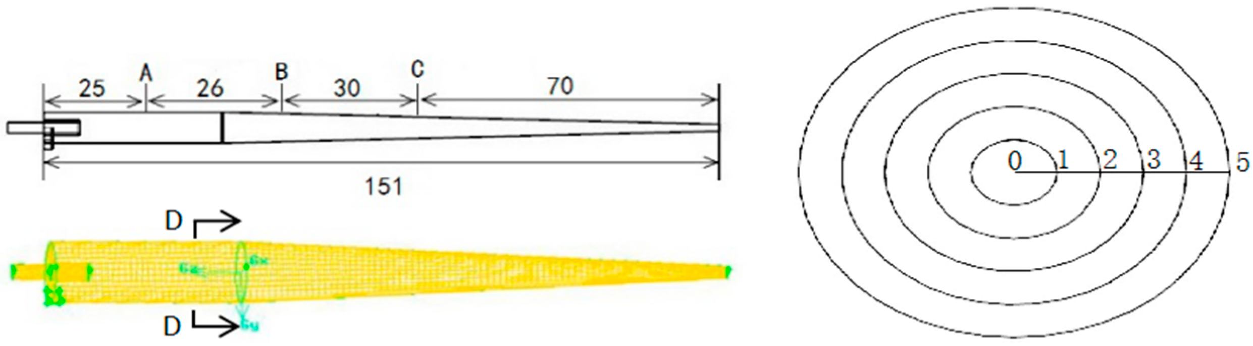
The parameters of the hydrocyclone used in this study were as follows. The diameters of the inlet, upstream, and downstream are 2, 3.4, and 2.2 mm, respectively. The cylinder section was 40 mm in height and 10 mm in diameter. The cone angle was 4 degrees. The shape and mesh conditions are shown in Figure 1. Based on the separation characteristics of hydrocyclones, it is generally believed that the sand particles moving against the wall where the cylinder and cone connect can be separated from the downstream. Therefore, the D-D section was set on the model to divide the area between the radial center and the wall into five regions. Figure 1a shows the model segmentation and meshing, and Figure 1b provides a magnified view of the D-D section 1:5. The three-dimensional structure was drawn using the UG10.0 (Unigraphics NX10.0) software, the meshing was done using the GAMBIT 2.4.6 software, and the numerical simulation was based on the ANSYS 16.0 and DEM 2.6.1 coupling method.

2.2. Numerical Simulation

2.2.1. Particle Characteristics

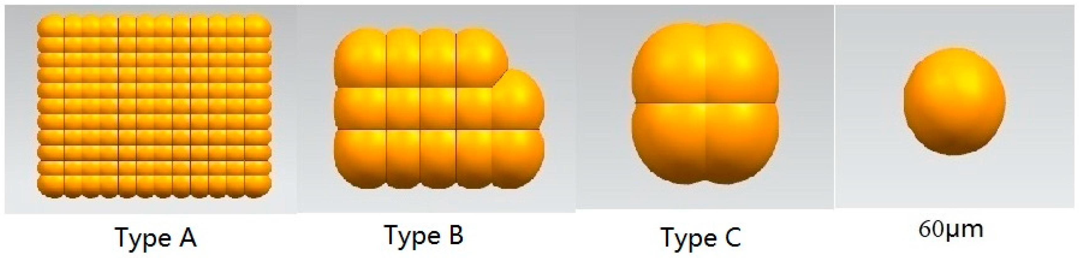
In this study, a single separation simulation of five spherical sand particles with diameters of 60, 70, 90, 106, and 120 µm was performed. A single separation simulation was conducted on three plate-like particles with the same volume as spherical sand particles of 60 µm (in Figure 2, the maximum projected area is S), and their maximum projected area was 3.11 S (type A), 2.24 S (type B), and 1.36S (type C), respectively. A mixed separation simulation was conducted on spherical sand particles with diameters of 60 and 120 µm.

Table 1. Parameters of particles in the numerical simulation.

Title 1	Type A	Type B	Type C	60 µm	70 µm	90 µm	106 µm	120 µm
Mass (μg)	0.28	0.28	0.28	0.28	0.44	0.95	1.54	2.23
Thickness (mm)	0.015	0.030	0.045	0.060	0.070	0.090	0.106	0.120
Maximum projected area (S)	3.11	2.24	1.36	1.00	1.36	2.24	3.11	4.00

shows the deformation amount, thickness, maximum projected area, and equivalent diameters of particles are shown in Table 1. The type C, B, and A particles share the maximum projected area with particles of 70 µm, 90 µm, and 106 µm, respectively.

In simulation experiments, the recorded residence time of sand particles in the cyclone equaled the period from their entering the inlet to their leaving the downstream or upstream. The data of particle velocity, position, and time were exported from the software DEM and edited by the MATLAB 2017b (Matrix Laboratory) postprocessor program. The values between the third and fourth seconds were collected as the analysis data.

2.2.2. Mathematical Model and Simulation Method

Flow in the hydrocyclone is considered to be an incompressible viscous fluid. The effect of gravity and the roughness of the hydrocyclone walls were taken into account, though surface tension was neglected. In the present study, the inlet velocity of the hydrocyclone was 2.00 m s⁻¹, The continuous medium flow is calculated from the continuity and the Navier–Stokes equations based on the local mean variables over a computational cell, which are given by:

$$\frac{\partial \mathsf{\epsilon }}{\partial \mathrm{t}}+\nabla ·\left(\mathsf{\epsilon }\mathrm{u}\right)=0$$

(1)

$$\frac{\partial \left({\mathsf{\rho }}_{\mathrm{f}}\mathsf{\epsilon }\mathrm{u}\right)}{\partial \mathrm{t}}+\nabla ·\left({\mathsf{\rho }}_{\mathrm{f}}\mathsf{\epsilon }\mathrm{uu}\right)=-\nabla \mathrm{P}-{\mathrm{F}}_{\mathrm{p}-\mathrm{f}}+\nabla ·(\mathsf{\epsilon }\mathsf{\tau })+{\mathsf{\rho }}_{\mathrm{f}}\mathsf{\epsilon }\mathrm{g}$$

(2)

F_p−f is Interaction forces between fluid and solid phases, equal to ${\displaystyle \sum _{\mathrm{i}=1}^{{\mathrm{k}}_{\mathrm{c}}}{\mathrm{f}}_{\mathrm{P}-\mathrm{f},\mathrm{i}}/\Delta {\mathrm{V}}_{\mathrm{c}}, \mathrm{N}/{\mathrm{m}}^3}$; the flow solved in Equations (1) and (2) represents the mixture flow of medium and sand, and was obtained by use of the models in a commercial ANSYS software package, i.e., Fluent. The details of the medium flow calculation and its validation can be found elsewhere [13,14]. In this work, we only give an overall description of the ANSYS model for the hydrocyclone.

The governing equations that are described above were discretized by the control volume numerical technique, and then the SIMPLE pressure–velocity coupling technique, with a second-order upwind scheme for the convection terms that were employed to solve the discretized equations over the computational domain.

The maximum particle volume fraction for the sand used in this study was less than 1%, which means the mixture of water and sand belonged to dilute phase flow. The Lagrangian coupling method was employed and

Table 2. Parameters used in the model.

Phase	Parameter	Symbol	Units	Value
Solid	Density distribution	ρ	kg·m−3	2500
	Rolling friction coefficient	μr	-	0.01
	Sliding friction coefficient	μs	-	0.30
	Poisson’s ratio	V	-	0.40
	Young’s modulus	E	N·m−2	2 × 10−7
	Coefficient of Restitution	cr	-	0.55
fluid	Density	ρ	kg·m−3	998.20
	Viscosity	μ	kg·m−1·s−1	0.001

summarizes the parameter settings for the sand [15],

Table 3. Boundary condition.

	Symbol	Units	Value
Particle velocity at inlet	v	m·s−1	2.00
Viscosity of Water Phase	v	m·s−1	2.00
Turbulent intensity	I	-	5%
Hydraulic radius	D	mm	2.00
Pressure at upstream	-	Pa	0.00
Pressure at downstream	-	Pa	0.00
Back-flow turbulence intensity	Ih	-	5%
Number of particle	-	N·s−1	1000
Particle diameter	di	μm	-

summarizes the boundary condition in the model. Ansys16.0 and DEM2.6.1 were employed during this study. The discrete approach was used to simulate sand movement, collisions among sand particles and between the sand particle and the hydrocyclone wall, and the effects of sand movement on the surrounding continuous phase, energy and momentum exchange. Collisions among sand particles and between sand particles and the wall did not lead to significant plastic deformation, which in consequence were attributed to hard particle contact, which is a wet grain contact model. The ‘Hertz-Mindlin (no slip) built-in’ model was utilized in this work [16].

In the simulation, the contributions of viscous drag force, pressure gradient force and gravity were considered. Other additional forces such as virtual mass force and Saffman force were not considered, as they are an order of magnitude smaller compared with the foregoing [17].

The CFD-DEM coupling process is described as follows: the continuous phase is resolved by ANSYS to acquire fluid drag force with sand, which was transformed from flow field information through the drag force model. The stress state of sands was measured by DEM to obtain new information such as the position and velocity of sands and to the flow field. ANSYS was used to model the flow and the most representative stress condition of sediments. The two approaches were coupled with a compound model that included the particle–fluid interaction force [16]. The relevant equations can be seen in

Table 4. Equations and specifications.

S/N	Name	Formula	Description
1	The normal force (Fn)	${\mathrm{F}}_{\mathrm{n}}=\frac{4}{3}{\mathrm{E}}^{\ast }{\left({\mathrm{R}}^{\ast }\right)}^{\raisebox{1ex}{$1$}\!\left/ \!\raisebox{-1ex}{$2$}\right.}{\mathsf{\alpha }}^{\raisebox{1ex}{$3$}\!\left/ \!\raisebox{-1ex}{$2$}\right.}$	R* is the equivalent radius α is the normal overlap
2	The equivalent elastic modulus (E*)	$\frac{1}{{\mathrm{E}}^{\ast }}=\frac{1-{\mathrm{V}}_1^2}{{\mathrm{E}}_1}+\frac{1-{\mathrm{V}}_2^2}{{\mathrm{E}}_2}$	E1, v1 and E1, v1 are elastic modulus and Poisson’s ratio of sand 1 and sand 2
3	The damping force (Fnd)	${\mathrm{F}}_{\mathrm{n}}^{\mathrm{d}}=-2\sqrt{\frac{5}{6}}\mathsf{\beta }\sqrt{{\mathrm{S}}_{\mathrm{n}}{\mathrm{m}}^{\ast }}{\mathrm{V}}_{\mathrm{n}}^{\mathrm{rel}}$	${\mathrm{V}}_{\mathrm{n}}^{\mathrm{rel}}$ is the normal relative velocity; Sn is the normal stiffness β is coefficient
4	The equivalent mass (m*)	${\mathrm{m}}^{\ast }=\frac{{\mathrm{m}}_1{\mathrm{m}}_2}{{\mathrm{m}}_1+{\mathrm{m}}_2}$	m1 and m2 are the mass of sand 1 and sand 2
5	The tangential force among the sands (Ft)	${\mathrm{F}}_{\mathrm{t}}=-{\mathrm{S}}_{\mathrm{t}}\mathsf{\delta }$	δ is the tangential overlap
6	The tangential stiffness (St)	${\mathrm{S}}_{\mathrm{t}}={8\mathrm{G}}^{\ast }\sqrt{{\mathrm{R}}^{\ast }\mathsf{\alpha }}$
7	The equivalent shear modulus (G*)	${\mathrm{G}}^{\ast }=\frac{2-{\mathrm{V}}_1^2}{{\mathrm{G}}_1}+\frac{2-{\mathrm{V}}_2^2}{{\mathrm{G}}_2}$	G1 and G2 are shear modulus of sand 1 and sand 2
		-	V1 and V2 are velocity of sand 1 and sand 2
8	The tangential damping force among sand particles (Ft)	${\mathrm{F}}_{\mathrm{t}}=-2\sqrt{\frac{5}{6}}\mathsf{\beta }\sqrt{{\mathrm{S}}_{\mathrm{t}}{\mathrm{m}}^{\ast }}{\mathrm{V}}_{\mathrm{t}}^{\mathrm{rel}}$	${\mathrm{V}}_{\mathrm{t}}^{\mathrm{rel}}$ is the tangential relative velocity
9	The rolling friction (Ti)	${\mathrm{T}}_{\mathrm{i}}=-{\mathsf{\mu }}_{\mathrm{r}}{\mathrm{F}}_{\mathrm{n}}{\mathrm{R}}_{\mathrm{i}}{\mathsf{\omega }}_{\mathrm{i}}$	μr is coefficient of rolling friction Ri is the distance between the center of mass to the point of contact; ωi is unit angular velocity vector of object at the contact point

.

Particle–fluid interaction, force (f_p−f, _i):

$$\begin{array}{l}{\mathrm{f}}_{\mathrm{D},\mathrm{i}}={(0.63+\frac{4.8}{{\mathrm{Re}}_{\mathrm{p},\mathrm{i}}^{0.5}})}^2\frac{{\mathsf{\rho }}_{\mathrm{f}}|{\mathrm{u}}_{\mathrm{i}}-{\mathrm{v}}_{\mathrm{i}}|\left(|{\mathrm{u}}_{\mathrm{i}}-{\mathrm{v}}_{\mathrm{i}}|\right)}{2}\frac{{\mathsf{\pi }\mathrm{d}}_{\mathrm{i}}^2}{4}{\mathsf{\epsilon }}_{\mathrm{i}}^{-\mathsf{\beta }}\\ {\mathrm{Re}}_{\mathrm{p},\mathrm{i}}=\frac{{\mathrm{d}}_{\mathrm{i}}{\mathsf{\rho }}_{\mathrm{f}}{\mathsf{\epsilon }}_{\mathrm{i}}|{\mathrm{u}}_{\mathrm{i}}-{\mathrm{v}}_{\mathrm{i}}|}{{\mathsf{\mu }}_{\mathrm{f}}},\mathsf{\beta }=3.7-0.65\exp \left[-\frac{{(1.5-{\mathrm{logRe}}_{\mathrm{p},\mathrm{i}})}^2}{2}\right]\\ \mathsf{\epsilon }=1-\frac{{\displaystyle \sum _{\mathrm{i}=1}^{{\mathrm{k}}_{\mathrm{C}}}{\mathrm{V}}_{\mathrm{i}}}}{{\Delta \mathrm{V}}_{\mathrm{C}}}\end{array}$$

(3)

$${\mathrm{f}}_{\mathrm{pg},\mathrm{i}}={\mathrm{V}}_{\mathrm{p},\mathrm{i}}\nabla \mathrm{P}$$

(4)

The free settling velocity (u_t)

$${\mathrm{u}}_{\mathrm{t}}=\frac{{\mathrm{gd}}^2}{18\mathsf{\upsilon }}\left(\frac{{\mathsf{\rho }}_{\mathrm{p}}-\mathsf{\rho }}{\mathsf{\rho }}\right)$$

(5)

Here, the drag coefficient (C) is

$$\mathrm{C}=\frac{\left({\mathsf{\rho }}_{\mathrm{P}}-\mathsf{\rho }\right)\mathrm{Vg}}{\mathrm{A}\mathsf{\rho }\left(\frac{{\mathrm{u}}^2}{2}\right)}$$

(6)

And the particle Reynolds number (Re) is

$$\mathrm{Re}=\frac{{\mathrm{D}}_{1\mathrm{p}}\mathrm{u}\mathsf{\rho }}{\mathsf{\mu }}$$

(7)

The drag coefficient varies depending on the inverse of the particle Reynolds number, thus the approximated drag coefficient was calculated as a function of the particle Reynolds number. The approximated drag coefficient Ca is expressed as

$${\mathrm{C}}_{\mathrm{a}}={\mathrm{C}}_0+{\mathrm{C}}_1\left(\frac{1}{\mathrm{Re}}\right)$$

(8)

and C₀ and C₁ were determined from the correlation of the particle Reynolds numbers and measured drag coefficients using the ratio of the particle diameter D₂ to thickness T as the particle shape factor

$${\mathrm{C}}_0=0.4555\mathrm{Ln}\left(\frac{{\mathrm{D}}_2}{\mathrm{T}}\right)+0.4687$$

(9)

$${\mathrm{C}}_1=19.285$$

(10)

Finally, the approximated drag coefficient was expressed as [18]:

$${\mathrm{C}}_{\mathrm{a}}=19.285\left(\frac{1}{\mathrm{Re}}\right)+0.4555\mathrm{Ln}\left(\frac{{\mathrm{D}}_2}{\mathrm{T}}\right)+0.4687$$

(11)

Pressure gradient force [19]: Due to the uneven distribution of hydraulic pressure on the surfaces of particles, the force is given by:

$${\mathrm{F}}_{\mathrm{p}}=-\frac{\nabla \mathrm{p}}{{\mathsf{\rho }}_{\mathrm{p}}}$$

(12)

The total drag force of fluid on sand particles (F_D)

$${\mathrm{F}}_{\mathrm{D}}={\mathsf{\xi }\mathrm{A}}_{\mathrm{p}}\frac{{\mathsf{\rho }\mathsf{\mu }}^2}{2}$$

(13)

When a particle accelerates in the viscous fluid, it will cause the surrounding fluid to accelerate, too. Due to the inertia effect, the fluid has a reaction force to the particle, which makes the inertia of the particle virtually increase. The related force is given by [2]:

$${\mathrm{F}}_{\mathrm{A}}=\frac{1}{2}\frac{\mathsf{\rho }}{{\mathsf{\rho }}_{\mathrm{p}}}\left(\frac{\mathrm{du}}{\mathrm{dt}}-\frac{{\mathrm{du}}_{\mathrm{p}}}{\mathrm{dt}}\right)$$

(14)

When a particle moves in a flow field with velocity gradient, it will experience a lateral force from the low flow rate side to the high flow rate side, given by:

$${\mathrm{F}}_{\mathrm{S}}=\frac{9.69}{{\mathsf{\pi }\mathrm{d}}_{\mathrm{p}}{\mathsf{\rho }}_{\mathrm{p}}}{\left(\mathsf{\mu }\mathsf{\rho }\left|\mathsf{\gamma }\right|\right)}^{\frac{1}{2}}{\mathrm{C}}_{\mathrm{LS}}\left(\mathrm{u}-{\mathrm{u}}_{\mathrm{p}}\right)$$

(15)

when a particle rotates at an angular velocity of ω, a lateral force perpendicular to the relative velocity and the rotation axis of the particle is generated from the upstream side to the downstream side, given by:

$${\mathrm{F}}_{\mathrm{M}}=\frac{3}{4}\frac{\mathsf{\rho }}{{\mathsf{\rho }}_{\mathrm{p}}}\frac{{\left(\mathrm{u}-{\mathrm{u}}_{\mathrm{p}}\right)}^2}{{\mathrm{d}}_{\mathrm{p}}}{\mathrm{C}}_{\mathrm{LM}}\frac{{\mathsf{\omega }}_{\mathrm{r}}\times {\mathrm{u}}_{\mathrm{r}}}{\left|{\mathsf{\omega }}_{\mathrm{r}}\right|\left|{\mathrm{u}}_{\mathrm{r}}\right|},{\mathsf{\omega }}_{\mathrm{r}}=\mathsf{\omega }-\mathsf{\Omega }$$

(16)

When a particle moves in a viscous fluid, the boundary layer on the surface of the particle will carry a certain amount of fluid. Due to the inertia of the fluid, the fluid cannot immediately follow the acceleration or deceleration of the particle, so this boundary layer is unstable, and the particle will be affected by a time-dependent force, given by:

$${\mathrm{F}}_{\mathrm{B}}=\frac{9}{{\mathrm{d}}_{\mathrm{p}}{\mathsf{\rho }}_{\mathrm{p}}}\sqrt{\frac{\mathsf{\rho }\mathsf{\mu }}{\mathsf{\pi }}}{\displaystyle {\int }_{{\mathrm{t}}_0}^{\mathrm{t}}\frac{\left(\mathrm{du}/\mathrm{d}\mathsf{\tau }\right)-\left({\mathrm{du}}_{\mathrm{p}}/\mathrm{d}\mathsf{\tau }\right)}{\sqrt{\mathrm{t}-\mathsf{\tau }}}}\mathrm{d}\mathsf{\tau }$$

(17)

In the Lagrangian coordinate system, the motions of particles are predicted based on the forces acting on them. In our studied system, the governing equation of particles can be given by

$$\frac{{\mathrm{du}}_{\mathrm{p}}}{\mathrm{dt}}=\left(1-\frac{\mathsf{\rho }}{{\mathsf{\rho }}_{\mathrm{p}}}\right)\mathrm{g}+{\mathrm{F}}_{\mathrm{D}}+{\mathrm{F}}_{\mathrm{P}}+{\mathrm{F}}_{\mathrm{A}}+{\mathrm{F}}_{\mathrm{S}}+{\mathrm{F}}_{\mathrm{M}}+{\mathrm{F}}_{\mathrm{B}}$$

(18)

The formula for the separation effect of the hydrocyclone:

$$\begin{array}{l}{\mathrm{P}}_{\mathrm{downstream}}=\frac{{\mathrm{N}}_{\mathrm{downstream}}}{{\mathrm{N}}_{\mathrm{downstream}}+{\mathrm{N}}_{\mathrm{upstream}}}\%\\ {\mathrm{P}}_{\mathrm{upstream}}=\frac{{\mathrm{N}}_{\mathrm{upstream}}}{{\mathrm{N}}_{\mathrm{downstream}}+{\mathrm{N}}_{\mathrm{upstream}}}\%\end{array}$$

(19)

2.3. Separation Experiments

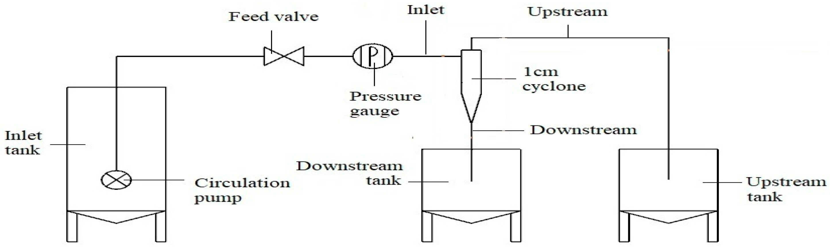
Figure 3 provides the flow chart of separation experiment in the hydrocyclone. The water pressure was controlled at 20 kPa by adjusting the feed valve (consistent with the pressure set in numerical simulation).

Sand particles with D50 of 120 µm were screened using a 115 to 125 mesh screen to substitute the 120 µm particles in numerical simulation, and particles with D50 of 60 µm were screened using a 230 to 250 mesh screen to substitute the 60 µm particles in numerical simulation.

The volume of 120 µm particles was eight times that of 60 µm particles. The volume of 120 µm particles put into the hydrocyclone was eight times that of 60 µm particles to ensure an equal number of both particles.

Table 5. Experiments for particle separation.

Particles	Particle Size (µm)	Concentration (kg·m−3)	Separation Time (s)
Singe	60	5	16
	120	40	16
Mixed	60 + 120	5 + 40	16

shows the standard volume concentration adopted. The concentrations for 60 and 120 µm particles were 5 kg·m⁻³ and 40 kg·m⁻³, respectively.

Experiment 1.

Sand particles (61–106 µm; 9 kg) were screened out using a 150 to 240 mesh screen to substitute the 60 to 106 µm irregular particles in numerical simulation, and a separation simulation was performed on them.

Experiment 2.

Three experiments were carried out, including two independent single separations of 60 and 120 µm particles and one mixed separation of both particles.

3. Analysis of Experimental Results

3.1. Flow Field, Flow Rate and Particle Distribution

The separation process of water and sand in a hydrocyclone is as follows: the turbulent flow of water drives the sediment particles to move, as a result of which the latter eventually flow out from the upstream and downstream separately. It can be seen that turbulent flow of water plays an important role in the separation of sediment particles. After it flows in from the inlet, the water flows into a swirling turbulent flow in the cavity, and finally carries the sediment particles out of the upstream or downstream separately.

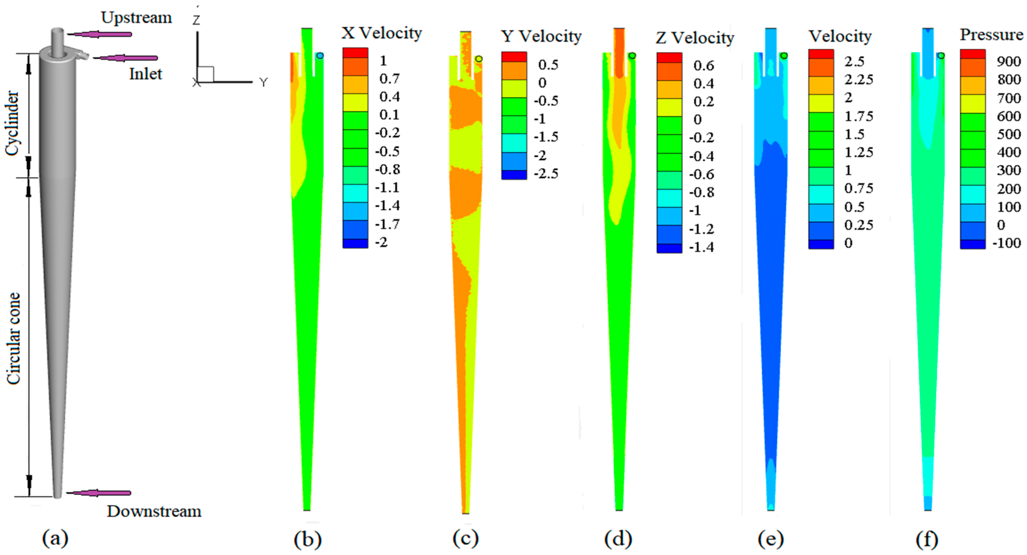
Figure 4 shows the velocity of water flow in the hydrocyclone along the X-, Y- and Z-axes, the resultant velocity of water flow (scalar quantity obtained by calculating the values of three coordinate axis), and the simulated result of water flow pressure distribution.

Figure 4a shows the structure of the hydrocyclone, Figure 4b, Figure 4c and Figure 4d are the water flow velocity (m/s) distributions along the X-, Y- and Z-axes, respectively. Figure 4e and Figure 4f presents the water flow velocity distribution and the water flow pressure distribution, separately. The velocity distribution along the X-axis is symmetrically distributed on both sides centered with the Z axis. The velocity distribution along the Y-axis exhibits periodic positive and negative phases. With regard to the speed distribution along the Z-axis, the velocity near the wall of the cylindrical section is low, and particles there flow from the downstream. The water flows through a zero-speed buffer zone when approaching the axis center, and eventually flows to the upstream. The general trend is that the water flow velocity in the cavity changes significantly at the intersection between cylinders, and the flow velocity increases near the downstream (as shown in Figure 4e). The pressure distribution in the cavity did not show obvious changes, but changes significantly when near the outlet. By observing the water flow velocity and pressure distribution, it can be known that the water flow carries the sediment particles from the inlet, and being blocked by the wall, particles rotate in circles in the cyclone chamber, and finally flow out from the upstream or the downstream. Since the water carrying capacity is influenced by the shape and size of the particles themselves, the hydrocyclone is usually used for sediment particle separation.

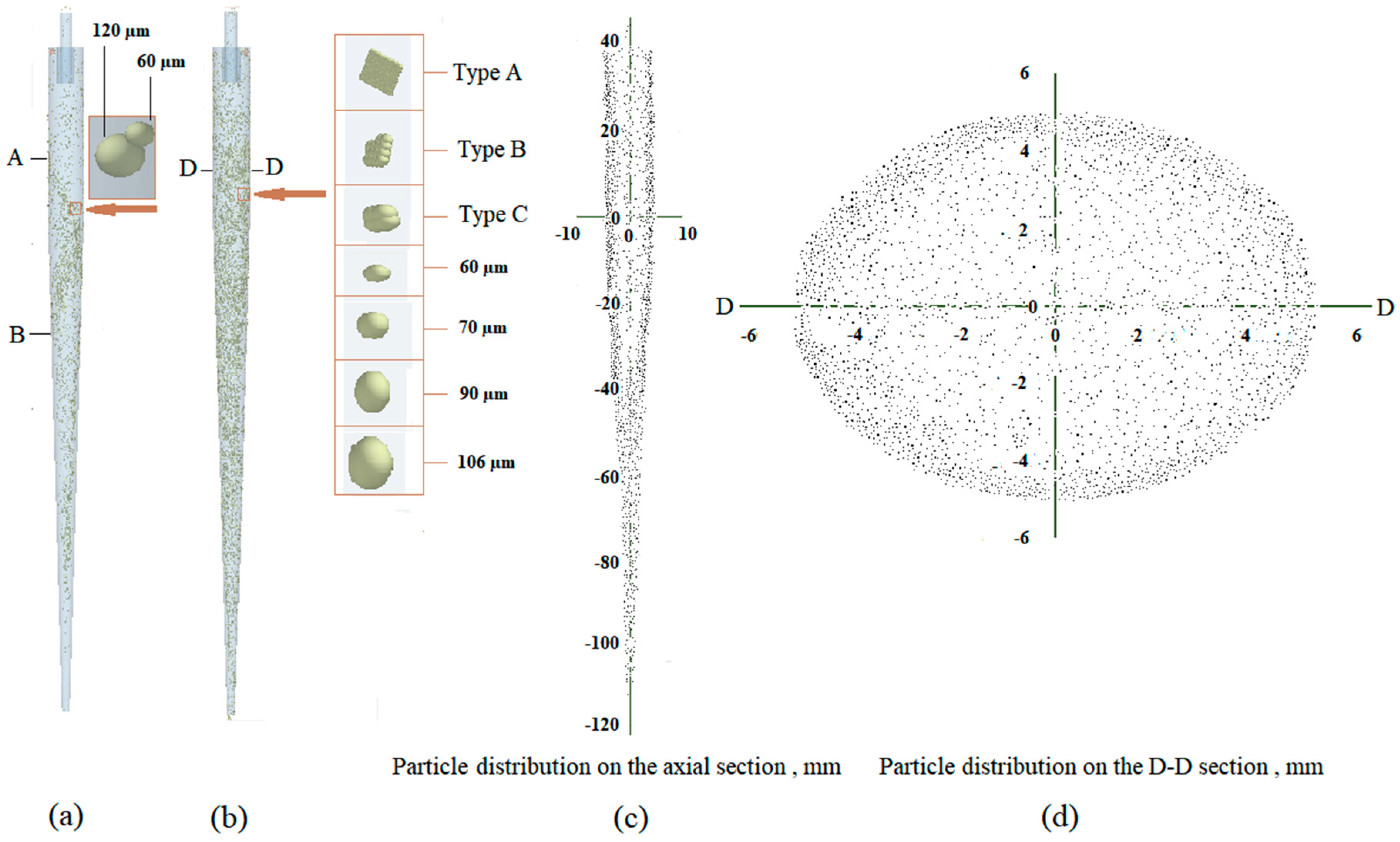
Figure 5 shows the position distribution of the particles in the hydrocyclone during the simulation. Figure 5a shows the separation simulation of 60 and 120 μm particles, and Figure 5b shows the simulation of the effect of the cross-section change of sand particles in the separation. Figure 5c shows the distribution of sand particles along the Z-axis and Figure 5d shows the particle distribution at the D-D section in Figure 5b.

From Figure 5c,d, the overall distribution of sand particle in the cylindrical section and part of the conical section can be obtained, and the closer of particles are to the wall, the higher the density is. The radial (X-axis) concentration distribution, as well as the velocity and the separation results in Figure 5b are shown in

Table 6. Concentration distribution of different sand particles in the cylindrical section.

Radial Distance	Type A	Type B	Type C	60 µm	70 µm	90 µm	106 µm
	Percentage of Content (%)
0–1	8.10	6.82	3.96	2.65	2.11	1.81	1.01
1–2	9.01	7.12	5.39	5.14	3.23	2.34	1.96
2–3	12.87	11.12	9.01	8.63	7.05	5.91	3.21
3–4	18.59	17.36	16.20	13.85	11.61	7.32	6.89
4–5	51.43	57.58	65.44	69.73	76.00	82.62	86.93

and

Table 7. Separation results of particles from the upstream.

Radial Distance	Maximum Projected Area (S)	tupstream (s)	tdownstream (s)	Vupstream (m s−1)	Vdownstream (m s−1)	Lupstream (m)	Ldownstream (m)	p (%)
Type A	3.11	0.63	2.21	0.41	0.59	0.26	1.30	24.0
Type B	2.24	0.66	2.15	0.41	0.59	0.27	1.27	17.8
Type C	1.36	0.69	2.11	0.41	0.59	0.28	1.25	14.9
60 µm	1.00	0.72	2.08	0.40	0.58	0.29	1.21	9.4
70 µm	1.36	0.75	2.02	0.39	0.59	0.29	1.19	7.4
90 µm	2.24	0.79	1.98	0.39	0.60	0.31	1.19	3.2
106 µm	3.11	0.81	1.92	0.39	0.60	0.32	1.15	0.9

t_upstream, the average residence time of particles crossing the upstream; t_downstream is the average residence time of particles crossing the downstream; V_upstream is the average absolute velocity of particles crossing the upstream; V_downstream is the average absolute velocity of particles crossing the downstream; L_upstream is the average path length of particles crossing the upstream; L_downstream is the average path length of particles crossing the downstream; and p is the percentage of the particles crossing the upstream in the separated particles, which was obtained using Equation (19).

, respectively. The axial velocity of the Z-axis, the radial (X-axis) distribution percentage, and the separation results in Figure 5a are shown in Figure 6,

Table 8. Concentration distribution of 60 and 120 µm particles in the cylinder section.

		0–1 mm	1–2 mm	2–3 mm	3–4 mm	4–5 mm
60 µm particles	Single	2.65	5.14	8.63	13.85	69.73
	Mixed	1.41	1.16	1.19	5.78	90.46
	Difference	−1.24	−3.98	−7.44	−8.07	20.73
120 µm particles	Single	1.33	1.50	1.64	2.30	93.23
	Mixed	1.21	1.32	1.79	2.95	92.73
	Difference	−0.12	−0.18	0.15	0.65	−0.5

and

Table 9. Separation of 60 and 120 µm particles.

		tavearge	Ndownstream	Nupstream	p (%)
Single	X	2.00	906	94	90.6
	D	1.70	1000	0	100
Mixed	X	1.80	947	53	94.7
	D	1.70	1000	0	100

X and D, the number of X (60 µm particles) and D (120 µm particles) was 1000 per second; t_avearge is the average time duration in which particles were separated from the downstream staying in the hydrocyclone in 3–4 s; N_downstream is the number of particles passing the downstream; N_upstream is the number of particles passing the upstream in 3–4 s; and p is the percentage of particles in the downstream, which was calculated using Formula (19).

, respectively.

3.2. Relationship between Maximum Projected Area and Separation Results

3.2.1. Radial Concentration Distribution of Particles

Table 6 shows the concentration distribution of different sand particles in the radial area of Figure 1. The general trend of sand particle distribution was that the higher the concentration distribution and the nearer the sands to the wall, the more concentrated the large sand particles, especially the 106 µm sand particles, which accounted for 86.93% of the total area.

The volume of 60 µm particles was the same as that of particle types C, B, and A. Their concentrations were 69.73%, 65.44%, 57.58%, and 51.43%, respectively, in the area with 4 to 5 mm radial distance near the wall. Therefore, the concentration of sand particles with the same volume tended to decrease gradually near the wall of the hydrocyclone with the increase in the maximum projected area.

The concentrations of 60, 70, 90, and 106 µm particles in the area with 4 to 5 mm radial distance were 69.73%, 76.00%, 82.62%, and 86.93%, respectively. That is to say, the concentration of spherical particles tended to increase in the direction of the hydrocyclone wall with the increase in the volume.

Taking the 2-3 area as the center, the concentrations of types C, B, and A in the area with 0 to 2 mm radial distance were 4.01%, 9.79%, and 14.14% higher than those of 70, 90, and 106 µm particles, respectively. Furthermore, their concentrations in the area with 3 to 5 mm radial distance were 5.97%, 15.00%, and 23.80% lower, respectively. Therefore, for the particles with the same volume and maximum projected area, the higher the concentration in the center of the hydrocyclone, the more likely the central part (the upwelling) flowing out from the upstream; for the particles with the same maximum projected area, the bigger the volume, the higher the concentration near the hydrocyclone wall, and the closer to the side wall, the more likely they might flow out from the downstream.

3.2.2. Separation Results in Numerical Simulation

Table 7 shows the separation results of the upstream and downstream with changes in the volume and maximum area.

As shown in Table 7, 9.4%, 7.4%, 3.2%, and 0.9% of spherical particles with diameters of 60, 70, 90, and 106 µm flowed out from the upstream, respectively. Therefore, it was harder for larger spherical particles to be separated from the upstream. The 60 µm particles had the same volume as types C, B, and A particles. As the maximum projected area increased gradually, 9.4%, 14.9%, 17.8%, and 24% of them flowed out from the upstream, accordingly. Thus, it was easier for the particles with the same volume to be separated from the upstream as the maximum projected area increased.

The 60 µm particles and types C, B, and A particles flowed out from the upstream in less time and traveled a shorter distance with the increase in the maximum projected area. For instance, the particles of type A took 0.09 s less compared with 60 µm particles and the average distance decrreased by 0.03 m.

However, the 60, 70, 90, and 106 µm particles needed more time to flow out from the upstream and travel a longer distance with the increase in their size. Among them, the 106 µm particles took the most time, 0.09 s more compared with 60 µm particles on average, and the average distance increased by 0.03 m.

For particles obtained from the upstream, the average velocity of 60 µm spherical particles and types A, B, and C particles was greater than that of 70, 90, and 106 µm particles. However, the average velocity of particles obtained from the downstream was in contrast to those from the upstream. The absolute velocity of different particles was less than that of water flow. Therefore, the smaller the particles or the larger the projected area, the stronger the ability to flow.

3.3. Separation Mechanism of Single and Mixed Particles

3.3.1. Distribution of Axial Velocity and Radial Concentration

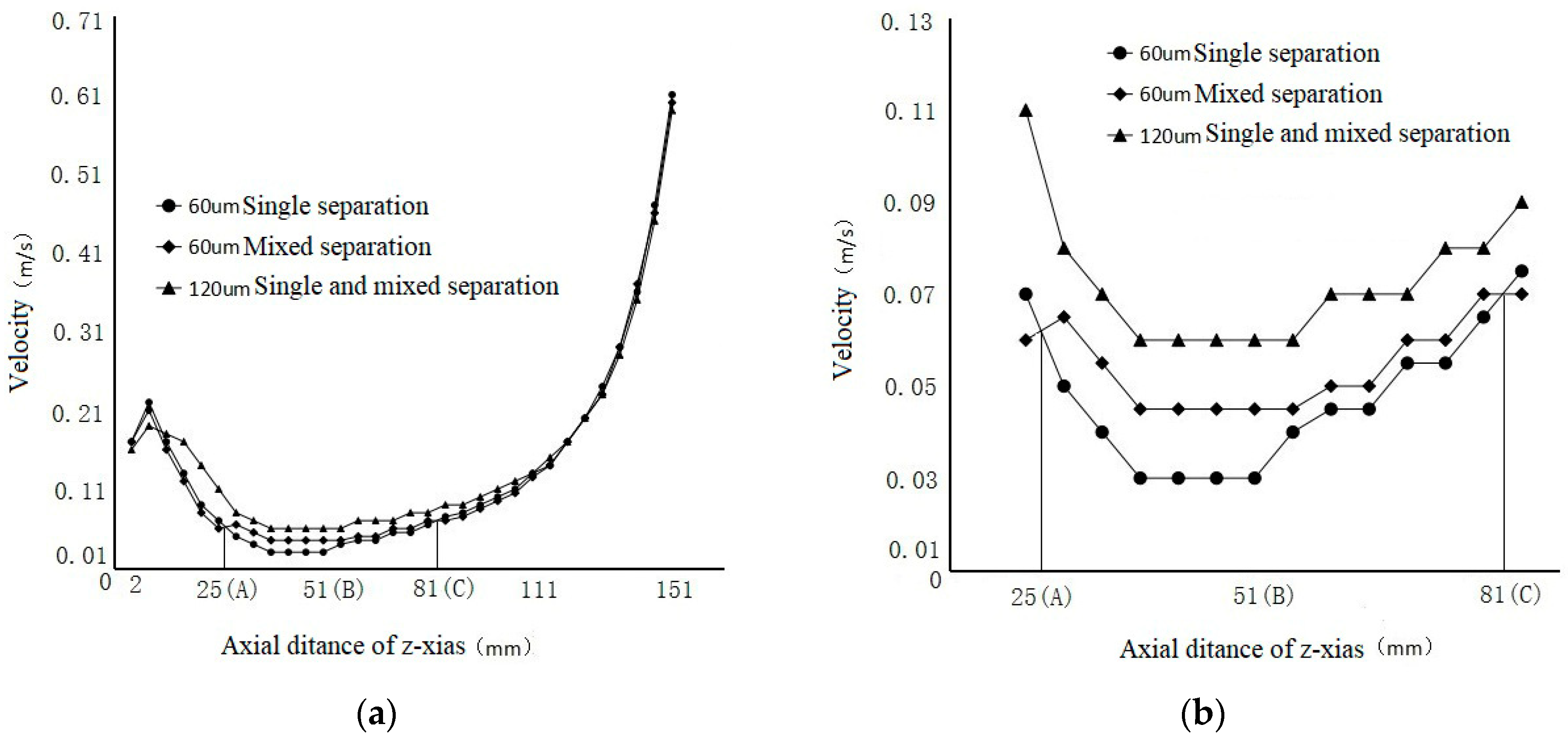
Figure 6 reflects the radial velocity of 60 and 120 µm particles. Three curves are seen from the top downward. The first one is about the average velocity of 120 µm particles in a positive direction, the direction of downstream. (The average velocity of 120 µm particles in single and mixed separations is shown by the same curve as it is the same in different separations, and 60 µm particles have no influence on 120 µm particles.) The second curve shows the average velocity of 60 µm particles in mixed separation in a positive direction (the direction of downstream). The third one is about the average velocity of 60 µm particles in single separation in a positive direction of Z axis. Figure 6b shows the partially enlarged image of Figure 6a (the former is five times bigger than the latter).

The velocity and direction of water flow significantly changed at 25–81 mm in Figure 6, which is the transition from a cylinder to a cone. Particles slowed down in a positive direction on the Z axis due to a lower water velocity, and the average velocity of different-sized particles also decreased. Thus, particles in this section mostly flow slowly in the whole separation process.

The velocity of 60 and 120 µm particles on Z axis had four changing stages: rising, falling, flattening, and rising again. Compared with a single separation, the average velocity of 60 µm particles increased by 25.74% at 25–81 mm in mixed separation, which was quite obvious at 25–51 mm. However, the velocity tended to be consistent at 0–25 mm and 81–151 mm.

The velocity was the lowest at 25–81 mm in the whole process. As shown in Figure 1, it was the border of cylinder and cone sections, 25–51 mm in the cylinder section and the rest in the cone section.

Table 8 shows the distribution of particle concentration at A to B in Figure 4. It was found that 93.23% of 120 µm particles in single separation were concentrated 4–5 mm away from the center of the circle in the radial direction. The percentage of particles nearest to the center of the circle was 1.33%. However, 69.73% of 60 µm particles in single separation were concentrated at 4–5 mm, and the percentage of particles nearest to the center of the circles was 2.65%. When the particles of these two sizes were mixed, the radial concentration distribution of 120 µm particles was in accordance with that of single separation generally. However, the radial concentration distribution of 60 µm particles in single separation was quite different from that of mixed separation. The difference was reflected in the section of 4–5 mm, and the percentage reached 20.73%.

In other words, influenced by 120 µm particles, 20.73% of 60 µm particles were concentrated in the aforementioned section in mixed separation.

3.3.2. Particle Separation Results

The calculation of particle separation took 4 s (see Table 9). The number of particles that flowed into the hydrocyclone was more than the sum of particles separated from upstream and desilting port in 0–3 s; the separation was unstable. However, it reached a dynamic balance because the number of particles flowing into the hydrocyclone was close to that of the particles separated from it in 3–4 s. When 60 µm particles were mixed with others, the average time spent in separation from the downstream was 0.2 s less than that in single separation while the separation increased by 4.1%. Furthermore, 120 µm particles were not separated in either single separation or mixed separation from the upstream.

4. Experimental Tests

4.1. Test on the Effect of Cross-Section Change on Separation

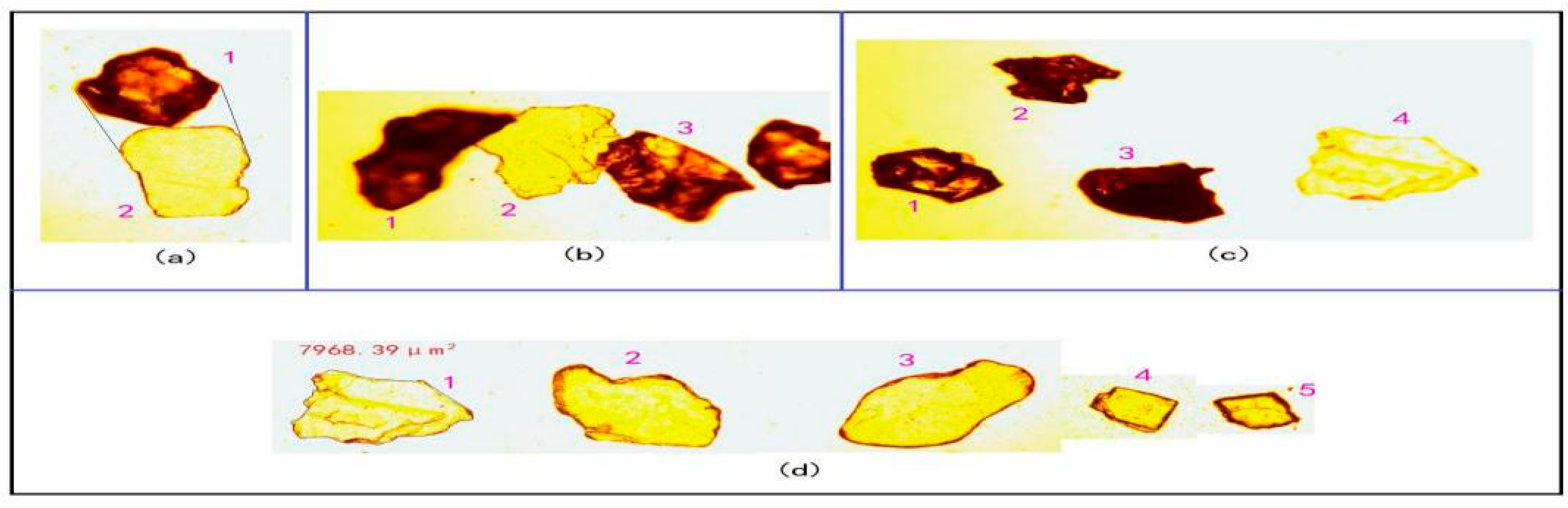
Figure 7 depicts the observation results of sand samples in the experiment. Figure 7a shows the representative sand particles screened using a vibrating screen. Both particles 1 and 2 could pass the 110 µm hydrocyclone screen, but they were not typical spherical particles, and their volume was less than that of spherical particles of the same size. Figure 7b shows the typical comparison of thickness. Obviously, particles 1 and 3 were thicker than particle 2 in terms of light transmittance. Figure 7c shows the particles with different projected area and thickness. Among them, the volumes of particles 1, 2, 3, and 4 might be the same. Figure 7d shows statistics on the maximum projected area of typical lamelliform particles separated from the upstream. The maximum projected area of particles 1, 2, 3, and 4 in Figure 4 was 7968.39, 8346.47, 8596.55, 3826.37, and 3949.87 µm², respectively. Accordingly, the size of spherical particles was 100.75, 103.11, 104.65, 69.81, and 70.93 µm, whose volume was less than that of spherical particles with the same projected area. Smaller particles were more than larger particles. Moreover, most were lamelliform particles with a similar size.

Different particles (10 groups) were observed with a transflective polarized microscope whose number was 59XC-PC before the experiment. It was found that most of 500 particles had a bad light transmittance and only a small number of them (10–30 particles) had a good light transmittance. However, about 160–210 among 500 particles obtained from the upstream were good in light transmittance (because they were relatively thin) after the experiment.

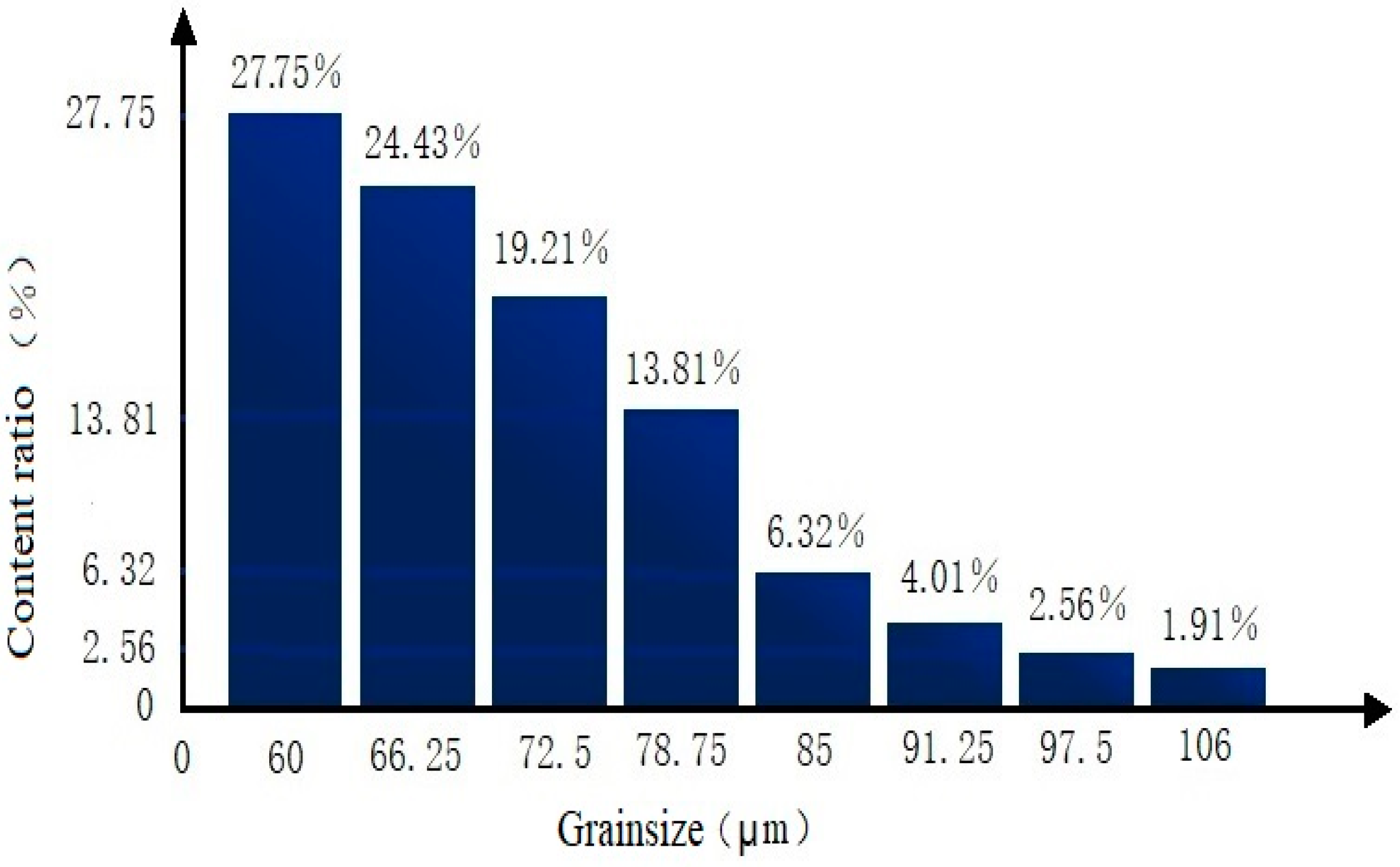
The results indicated that the larger the size of particles, the less the particles were separated from the upstream. As shown in Figure 8, the percentage of 60 and 106 µm particles was 27.75 and 1.91%, respectively.

Therefore, smaller and thinner particles were separated from the upstream more easily. In other words, the process of separating sand particles in the hydrocyclone led to the classification of particles of different sizes, which was equivalent to the filtering of particles of different shapes (lamelliform particles). The experimental result was consistent with the regularities reflected in numerical simulation.

4.2. Separation Test of Sand Particles 60 and 120 μm

The concentration of 60 and 120 µm sand particles was set as 5 kg·m⁻³ and 40 kg·m⁻³, respectively, to ensure an equal number of sand particles put into the hydrocyclone. The capacity of the container was 1 m³. The separation experiment lasted for 16 min.

Table 10. Separation experiments for 60 and 120 µm sand particles.

	Single		Mixed
	60 µm	120 µm	60 µm	120 µm
Upstream	0.312	0	0.255	0
Downstream	28.85		29.25

shows the results: 120 µm sand particles were separated from the downstream in both single and mixed separations. However, 312 g of 60 µm sand particles were separated from the upstream in single separation, and 255 g were separated in mixed separation. It was concluded that larger particles improved the separation of smaller ones from the upstream in mixed separation, which was consistent with the regularities reflected in numerical simulation.

5. Discussion

5.1. Influence of Maximum Projected Area and Volume Changes on Separation Results

Several parameters affect the performance of hydrocyclones, including the inlet velocity, solid content, liquid-phase viscosity, particle size and shape, and so forth. Saber et al. [20] believed that the separation effect would improve with the increase in the size of spherical particles, which was obviously better than that of plate-like particles. Also, the separation effect declined with the increase in the size of plate-like particles with diameters more than 60 µm. Abdollahzadeh et al. [21] thought that the separation effect decreased along with the increase in flatness when the particle diameter was more than 10 µm. Endoh et al. [22] found that particles with a large size and high proportion were separated from the upstream. Wills et al. [23] held the view that plate-like particles, such as mica, were often discharged upstream even though they were relatively coarse. Kashiwaya et al. [17] believed that the shape of particles would influence the drag coefficient and separation effect. The drag coefficient would increase when the particles became flatter. Then, the increased drag force would increase the influence of water movement on particles. Wang et al. [24] found that the change in particle velocity fluctuated evidently as the size of particles became smaller and the drag force increased. Some particles passed through the locus of zero vertical velocity, joined the upward flow, and then moved out from the upstream. In this study, particles of types C, B, and A, corresponding to 70, 90, and 106 µm particles, respectively, could enter the upward flow and then flow out of the upstream easily as particles became smaller and drag force increased. Therefore, the corresponding percentage dropped sharply in the area with 3 to 5 mm radial distance and increased in the area with 1 to 3 mm radial distance.

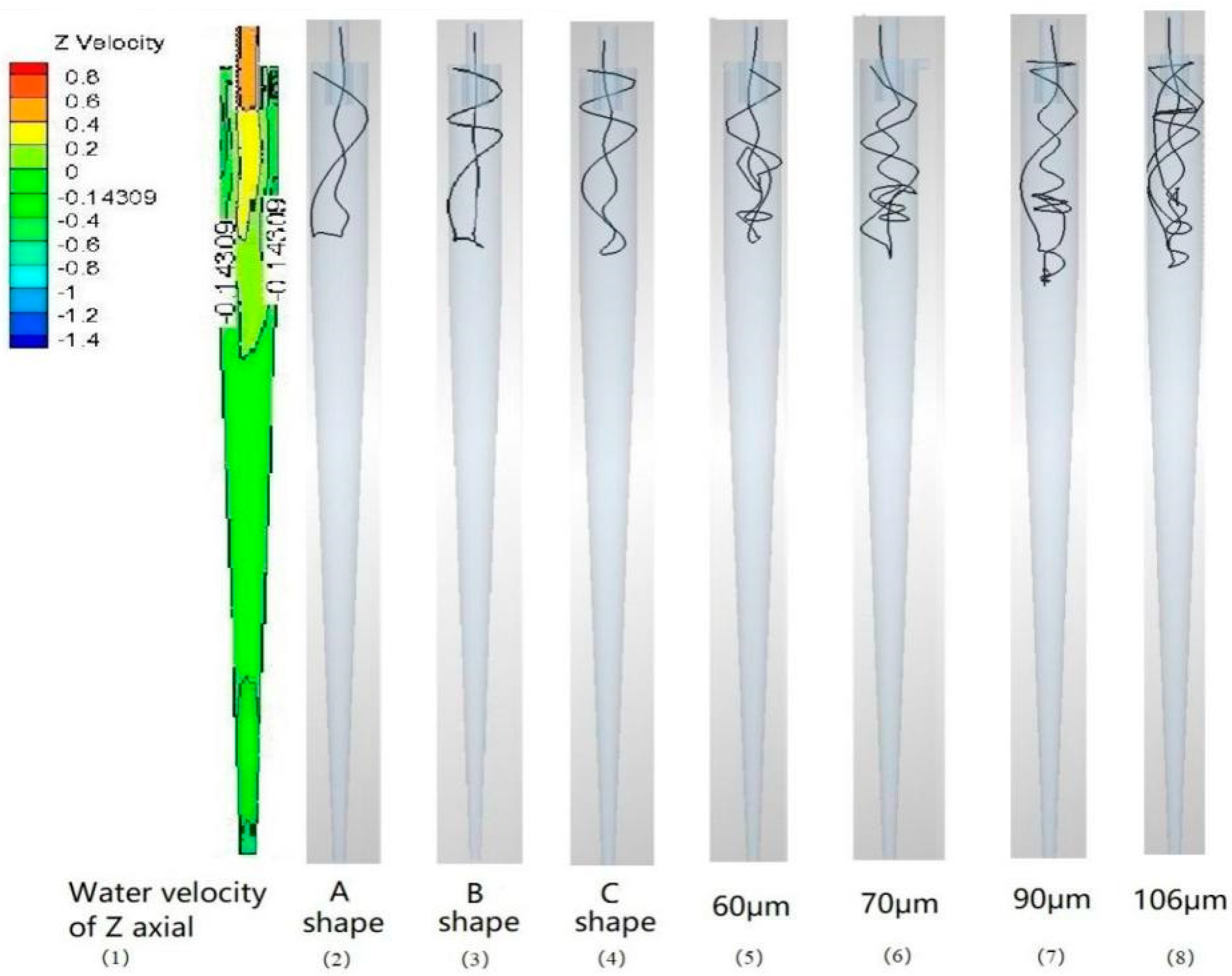
Drag force is proportional to the maximum projected area of particles along the direction of fluid flow (Formula (19)), which means that the drag force is strengthened with the increase in the maximum projected area of particles. Hence, the maximum projected area of particles has a certain influence on the separation results of the hydrocyclone. Kashiwaya et al. considered that when Reynolds number reached a certain level (above 50), the maximum projected area of particles was a major influencing factor. They also claimed that the radial variation in the tangential velocity in the hydrocyclone gave rise to a moment on plate-like particles and the particles settled, maintaining the orientation as their broad planes became perpendicular to the radial direction. In this study, the pressure gradient force in the upwelling direction toward the center of the hydrocyclone in the same position increased with the increase in the cross-sectional area. Also, the particles could be easily pushed into the upwelling and then out of the upstream. Figure 9 shows that the volume of 60 µm spherical particles was the same as that of particles of types C, B, and A, but the cross-sectional area was larger and hence the track was simpler in the hydrocyclone.

Figure 9 shows the representative motion tracks of sand particles with different cross-sectional areas when they moved from the upstream. The figure shows that 60 µm spherical particles had the same volume as that of particles of types C, B, and A. With the increase in the maximum projected area, the tracks became simpler and the time needed for separation became shorter. Furthermore, 60, 70, 90, and 106 µm particles were all spherical. The tracks separated from the upstream become more complex with the increase in the volume of particles. That is, it was harder for particles to separate from the upstream as the time taken for separation increased. Tracks (2) and (8), (3) and (7), and (4) and (6) belong to the particles with the same maximum projected area. The smaller the volume of particles, the simpler the tracks when separated from the upstream, indicating that the time taken for separation was shorter, and it was harder for particles to separate from the upstream. Hence, the maximum projected area might have an obvious and a stable influence on the motion tracks of particles, hence affecting the separation effect.

5.2. Analysis of the Following Phenomenon of Fine Particles

Zhang et al. [19] believed that the movement of particles was controlled by the combined effect of the radial fluid drag force, pressure gradient force, and centrifugal force. Of these, the fluid drag force of the inward direction increased exponentially with decreasing size of small particles. A part of the small particles was pushed into the center of the hydrocyclone and then flowed out of upstream. Xu et al. [25] held the view that large particles moved toward the wall under the effect of inertial force and gravity. In this test, a part of 60 µm particles flowed out of the upstream, while the 120 µm particles did not. However, the following phenomenon enhanced the density of the 60 µm particles near the wall, where most 120 µm sand particles were present, thereby reducing the possibility of 60 µm particles flowing into the center of the hydrocyclone and out of the upstream. Therefore, the force on particles in the hydrocyclone was complicated. Zhu et al. [26] noted that the comprehensive effect of the fluid drag force, pressure gradient force, virtual mass force, and gravity on particles should be taken into consideration. Peng et al. used the lattice Boltzmann method to successfully simulate the shallow water flows and river bed evolution [27,28,29,30,31,32,33,34] as well as two-phase flows [35,36].

Tsuji et al. [37] believed that the large leading particles had a huge drag force on small trailing particles, which had little or even no drag force on leading particles in turn. The experiment showed that 120 µm particles had a great impact on 60 µm particles in terms of distribution, velocity, or separation effect. However, no 120 µm particles separated from the upstream. Furthermore, 120 µm sand particles could influence 60 µm particles to a great degree, but the latter’s influence on the former could be neglected, which was consistent with the findings of other studies. Meanwhile, Zhu et al. [38] claimed that Re could affect drag, and the increase in Re could obviously weaken the influence of leading particles on small ones. Zhang et al. [18] held the view that the following drag of small particles toward large ones would decrease with the increasing distance, and it would be affected by particle’s ratio and the local wake flow compared with that between the particles and the incoming fluid stream. Schubert et al. [39] considered that this phenomenon was due to particle interaction, while the finer particles were captured by the larger particles and the effect was more prominent with the increase in the fraction of large particles. In this study, Re did not change at all under the force of inlet pressure, which was the only one used in this experiment. However, the following phenomenon was quite obvious from the perspectives of process and results.

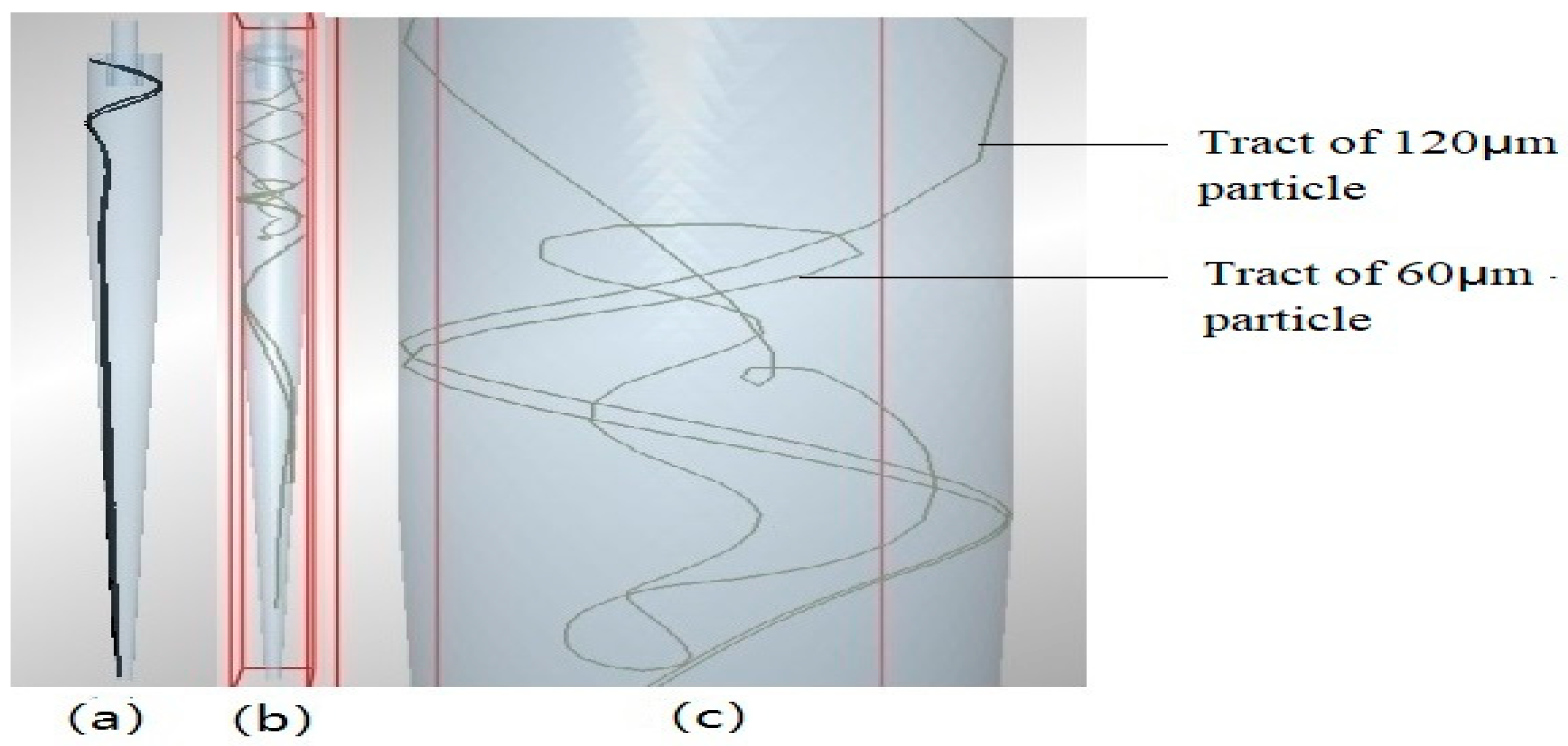
Under the ideal circumstances, the deposition velocity of spherical particles is proportional to particle diameter (Formula (13)). The velocity is high with the increase in the particle diameter. The numerical calculation and experimental results in this study showed that larger particles were faster than smaller particles in terms of deposition velocity in the hydrocyclone. CFD–DEM coupling was adopted to capture the following phenomena of the movement of small particles toward large ones (see Figure 10). Figure 10a,b presents the motion tracks of 120 and 60 µm particles in the downstream in mixed separation, whereas Figure 10c is the enlarged drawing of the complex segment in Figure 10b. In the figure, among particles around the transition section from a cylinder to a cone, 60 µm particles firstly entered the hydrocyclone, and their motion track was chaotic. After meeting with the 120 µm particles, the 60 µm particles changed their direction and were separated from the downstream together with the 120 µm ones. This phenomenon also explains why the average velocity of mixed separation of 60 and 120 µm particles near the boundary of cylinder and cone was higher than that of single separation (Figure 6).

6. Conclusions

In this study, numerical simulation and experimental methods were applied to reveal the separation mechanism of the hydrocyclone for different-sized particles and the influence of maximum projected area on the separation effect. The conclusions were as follows:

The percentage of 60, 70, 90, 106, and 120 µm spherical particles separated from the upstream was 9.4%, 7.4%, 3.2%, 0.9%, and 0%, respectively, indicating that spherical particles were more easily separated from the downstream as their size increased.

For 60 µm spherical particles and types C, B, and A particles with the same volume, the separation percentages from the upstream were 9.4%, 14.9%, 17.8%, and 24.0%, respectively, implying that the running space was closer to the upward flow in the hydrocyclone as the maximum projected area increased. Hence, particles with the same volume were easier to be separated from the upstream.

The axial velocity of 60 µm particles mixed with 120 µm particles in separation increased by 25.74% compared with that in the single separation of 60 µm particles near the transition section from a cylinder to a cone. The concentration near the wall, where mainly 120 µm particles were present, increased by 20.73%, and the separation effect in the downstream improved by 4.1%. Therefore, large particles could optimize the separation effect of small particles from the downstream.

References

- Fu, S.; Yong, F.; Yuan, H.; Tan, W.; Dong, Y. Effect of the medium’s density on the hydrocyclonic separation of waste plastics with different densities. Waste Manag. 2017, 67, 27–31. [Google Scholar] [CrossRef] [PubMed]
- Zhang, Y.; Cai, P.; Jiang, F.; Dong, K.; Jiang, Y.; Wang, B. Understanding the separation of particles in a hydrocyclone by force analysis. Powder Technol. 2017, 322, 471–489. [Google Scholar] [CrossRef]
- Neesse, T.; Dueck, J.; Schwemmer, H.; Farghaly, M. Using a high pressure hydrocyclone for solids classification in the submicron range. Miner. Eng. 2015, 71, 85–88. [Google Scholar] [CrossRef]
- Yu, L.; Zou, X.; Hong, T.; Yan, W.; Chen, L.; Xiong, Z. 3D numerical simulation of water and sediment flow in hydrocyclone based on coupled cfd-dem. Trans. Chin. Soc. Agric. Mach. 2016, 01, 126–132. [Google Scholar]
- Zhu, G.; Liow, J. Experimental study of particle separation and the fishhook effect in a mini-hydrocyclone. Chem. Eng. Sci. 2014, 111, 94–105. [Google Scholar] [CrossRef]
- Liu, H.; Wang, Y.; Han, T. Influence of vortex finder configurations on separation of fine particles. CIESC J. 2017, 05, 1921–1931. [Google Scholar]
- Tang, B.; Xu, Y.; Song, X.; Xu, J. Effect of inlet configuration on hydrocyclone performance. Trans. Nonferrous Met. Soc. China 2017, 27, 1645–1655. [Google Scholar] [CrossRef]
- Hwang, K.-J.; Chou, S.-P. Designing vortex finder structure for improving the particle separation efficiency of a hydrocyclone. Sep. Purif. Technol. 2017, 172, 76–84. [Google Scholar] [CrossRef]
- Vakamalla, T.R.; Koruprolu, V.B.R.; Arugonda, R.; Mangadoddy, N. Development of novel hydrocyclone designs for improved fines classification using multiphase cfd model. Sep. Purif. Technol. 2017, 175, 481–497. [Google Scholar] [CrossRef]
- Zhang, C.; Wei, D.Z.; Cui, B.Y.; Li, T.S.; Luo, N. Effects of curvature radius on separation behaviors of the hydrocyclone with a tangent-circle inlet. Powder Technol. 2017, 305, 156–165. [Google Scholar] [CrossRef]
- Zhou, Q.; Wang, C.; Wang, H.; Wang, J. Eulerian–lagrangian study of dense liquid–solid flow in an industrial-scale cylindrical hydrocyclone. Int. J. Miner. Process. 2016, 151, 40–50. [Google Scholar] [CrossRef]
- Zhao, Q.; Li, W.; He, W. Experimental study of pressure drop characteristics of a novel solid/liquid hydrocyclone. J. Eng. Thermophys. 2010, 01, 61–63. [Google Scholar]
- Wang, B.; Chu, K.W.; Yu, A.B. Numerical study of particle–fluid flow in a hydrocyclone. Ind. Eng. Chem. Res. 2007, 46, 4695–4705. [Google Scholar] [CrossRef]
- Wang, B.; Chu, K.W.; Yu, A.B.; Vince, A. Modelling the multiphase flow in a dense medium cyclone. Ind. Eng. Chem. Res. 2009, 48, 3628–3639. [Google Scholar] [CrossRef]
- Asakura, K.; Asari, T.; Nakajima, I. Simulation of solid–liquid flows in a vertical pipe by a collision model. Powder Technol. 1997, 94, 201–206. [Google Scholar] [CrossRef]
- Chu, K.W.; Wang, B.; Yu, A.B.; Vince, A. Cfd-dem modelling of multiphase flow in dense medium cyclones. Powder Technol. 2009, 193, 235–247. [Google Scholar] [CrossRef]
- Niu, W.; Liu, L.; Chen, X. Influence of fine particle size and concentration on the clogging of labyrinth emitters. Irrig. Sci. 2013, 31, 545–555. [Google Scholar] [CrossRef]
- Kashiwaya, K.; Noumachi, T.; Hiroyoshi, N.; Ito, M.; Tsunekawa, M. Effect of particle shape on hydrocyclone classification. Powder Technol. 2012, 226, 147–156. [Google Scholar] [CrossRef] [Green Version]
- Zhang, J.; Fan, L.S. A semianalytical expression for the drag force of an interactive particle due to wake effect. Ind. Eng. Chem. Res. 2002, 41, 5094–5097. [Google Scholar] [CrossRef]
- Niazi, S.; Habibian, M.; Rahimi, M. A comparative study on the separation of different-shape particles using a mini-hydrocyclone. Chem. Eng. Technol. 2017, 40, 699–708. [Google Scholar] [CrossRef]
- Abdollahzadeh, L.; Habibian, M.; Etezazian, R.; Naseri, S. Study of particle’s shape factor, inlet velocity and feed concentration on mini-hydrocyclone classification and fishhook effect. Powder Technol. 2015, 283, 294–301. [Google Scholar] [CrossRef]
- Endoh, S. Study of the shape separation of fine particles using fluid fields-dynamic properties of irregular shaped particles in wet cyclones. J. Soc. Powder Technol. Jpn. 1992, 29, 125–132. [Google Scholar] [CrossRef]
- Wills, B.A.; Napier-Munn, T. Wills’ Mineral Processing Technology, 7th ed.; Elsevier Science & Technology Books: Amsterdam, The Netherlands, 2006; pp. 145–206. [Google Scholar]
- Wang, B.; Yu, A.B. Computational investigation of the mechanisms of particle separation and “fish-hook” phenomenon in hydrocyclones. AIChE J. 2010, 56, 1703–1715. [Google Scholar] [CrossRef]
- Xu, P.; Wu, Z.; Mujumdar, A.S.; Yu, B. Innovative hydrocyclone inlet designs to reduce erosion-induced wear in mineral dewatering processes. Dry. Technol. 2009, 27, 201–211. [Google Scholar] [CrossRef]
- Zhu, C.; Liang, S.C.; Fan, L.S. Particle wake effects on the drag force of an interactive particle. Int. J. Multiph. Flow 1994, 20, 117–129. [Google Scholar] [CrossRef]
- Peng, Y.; Zhou, J.G.; Burrows, R. Modelling the free surface flow in rectangular shallow basins by lattice Boltzmann method. J. Hydraul. Eng. ASCE 2011, 137, 1680–1685. [Google Scholar] [CrossRef]
- Peng, Y.; Zhou, J.G.; Burrows, R. Modelling solute transport in shallow water with the lattice Boltzmann method. Comput. Fluids 2011, 50, 181–188. [Google Scholar] [CrossRef]
- Peng, Y.; Zhang, J.M.; Zhou, J.G. Lattice Boltzmann Model Using Two-Relaxation-Time for Shallow Water Equations. J. Hydraul. Eng. ASCE 2016, 142, 06015017. [Google Scholar] [CrossRef]
- Peng, Y.; Zhang, J.M.; Meng, J.P. Second order force scheme for lattice Boltzmann model of shallow water flows. J. Hydraul. Res. 2017, 55, 592–597. [Google Scholar] [CrossRef]
- Peng, Y.; Zhou, J.G.; Zhang, J.M.; Burrows, R. Modeling moving boundary in shallow water by LBM. Int. J. Mod. Phys. C 2013, 24, 1–17. [Google Scholar] [CrossRef]
- Peng, Y.; Zhou, J.G.; Zhang, J.M.; Liu, H.F. Lattice Boltzmann Modelling of Shallow Water Flows over Discontinuous Beds. Int. J. Numer. Method Fluids 2014, 75, 608–619. [Google Scholar] [CrossRef]
- Peng, Y.; Zhou, J.G.; Zhang, J.M. Mixed numerical method for bed evolution. Proc. Inst. Civ. Eng. Water Manag. 2015, 168, 3–15. [Google Scholar] [CrossRef]
- Peng, Y.; Meng, J.P.; Zhang, J.M. Multispeed lattice Boltzmann model with stream-collision scheme for transcritical shallow water flows. Math. Probl. Eng. 2017, 2017, 8917360. [Google Scholar] [CrossRef]
- Peng, Y.; Mao, Y.F.; Wang, B.; Xie, B. Study on C-S and P-R EOS in pseudo-potential lattice Boltzmann model for two-phase flows. Int. J. Mod. Phys. C 2017, 28, 1750120. [Google Scholar] [CrossRef]
- Peng, Y.; Wang, B.; Mao, Y.F. Study on force schemes in pseudopotential lattice Boltzmann model for two-phase flows. Math. Probl. Eng. 2018, 2018, 6496379. [Google Scholar] [CrossRef]
- Tsuji, Y.; Morikawa, Y.; Terashima, K. Fluid-dynamic interaction between two spheres. Int. J. Multiph. Flow 1982, 8, 71–82. [Google Scholar] [CrossRef]
- Zhu, G.; Liow, J.L.; Neely, A. Computational study of the flow characteristics and separation efficiency in a mini-hydrocyclone. Chem. Eng. Res. Des. 2012, 90, 2135–2147. [Google Scholar] [CrossRef]
- Schubert, H. On the origin of “Anomalous” shapes of the separation curve in hydrocyclone separation of fine particles. Part. Sci. Technol. 2004, 22, 219–234. [Google Scholar] [CrossRef]
Figure 1.
The axial length of Z axis and cross section of the cylinder of the hydrocyclone.
Figure 2.
Particle shapes in numerical simulation.
Figure 3.
Schematic diagram of the hydrocyclone test.
Figure 4.
Structure of the cyclone, water flow velocity (m·s−1) and pressure (Pa) distribution: (a) structure of hydrocyclone; (b) flow velocity in X-axis; (c) flow velocity in Y-axis; (d) flow velocity in Z-axis; (e) water flow velocity distribution; (f) water flow pressure distribution.
Figure 5.
Sand particle distribution in simulation: (a) the separation simulation of 60 and 120 μm particles; (b) the simulation of the effect of the cross-section change of sand particles in the separation; (c) the distribution of sand particles along the Z-axis; (d) the particle distribution at the D-D section in (b).
Figure 6.
Average velocity distribution in a positive direction of Z axis: (a) radial velocity of 60 and 120 µm particles; (b) partially enlarged image of (a).
Figure 7.
Distribution of particle characteristics (×1 k).
Figure 8.
Percentage of particles with different sizes on the upstream.
Figure 9.
Representative motion tracks of sand particles.
Figure 10.
Representative motion tracks of particles.