Sensitivity Analysis of a Wall Boundary Condition for the Turbulent Pipe Flow of Herschel–Bulkley Fluids
by

Dhruv Mehta
1,*,†, 
Adithya Krishnan Thota Radhakrishnan
1,
Jules Van Lier
1 and
Francois Clemens
1,2,‡
1
Sanitary Engineering, Faculty of Civil Engineering and Geosciences, Delft University of Technology, 2628 CN Delft, The Netherlands
2
Stichting Deltares, 2629 HV Delft, The Netherlands
*
Author to whom correspondence should be addressed.
†
Current address: Sanitary Engineering, Stevinweg 1, 2628 CN Delft, The Netherlands.
‡
This document is a follow-up study to Mehta et al. and is a collaborative effort.
Water 2019, 11(1), 19; https://doi.org/10.3390/w11010019
Submission received: 17 October 2018
/
Revised: 13 December 2018
/
Accepted: 19 December 2018
/
Published: 22 December 2018
(This article belongs to the Special Issue Smart Hydraulics in Wastewater Transport)
Abstract
:This article follows from a previous study by the authors on the computational fluid dynamics-based analysis of Herschel–Bulkley fluids in a pipe-bounded turbulent flow. The study aims to propose a numerical method that could support engineering processes involving the design and implementation of a waste water transport system, for concentrated domestic slurry. Concentrated domestic slurry results from the reduction in the amount of water used in domestic activities (and also the separation of black and grey water). This primarily saves water and also increases the concentration of nutrients and biomass in the slurry, facilitating efficient recovery. Experiments revealed that upon concentration, domestic slurry flows as a non-Newtonian fluid of the Herschel–Bulkley type. An analytical solution for the laminar transport of such a fluid is available in literature. However, a similar solution for the turbulent transport of a Herschel–Bulkley fluid is unavailable, which prompted the development of an appropriate wall function to aid the analysis of such flows. The wall function (called hereafter) was developed using Launder and Spalding’s standard wall function as a guide and was validated against a range of experimental test-cases, with positive results. is assessed for its sensitivity to rheological parameters, namely the yield stress, the fluid consistency index and the behaviour index and their impact on the accuracy with which can correctly quantify the pressure loss through a pipe. This is done while simulating the flow of concentrated domestic slurry using the Reynolds-Averaged Navier–Stokes (RANS) approach for turbulent flows. This serves to establish an operational envelope in terms of the rheological parameters and the average flow velocity within which is a must for accuracy. One observes that, regardless of the fluid behaviour index, is necessary to ensure accuracy with RANS models only in flow regimes where the wall shear stress is comparable to the yield stress within an order of magnitude. This is also the regime within which the concentrated slurry analysed as part of this research flows, making a requirement. In addition, when the wall shear stress exceeds the yield stress by more than one order (either due to an inherent lower yield stress or a high flow velocity), the regular Newtonian wall function proposed by Launder and Spalding is sufficient for an accurate estimate of the pressure loss, owing to the relative reduction in non-Newtonian viscosity as compared to the turbulent viscosity.
The research described in this article is aimed at experimentally and numerically supporting the design of a novel sanitation system for urban areas with emphasis on the separation of black water from toilets and grey water from kitchen and washing, in order to facilitate a decentralised recovery of nutrients and biomass. This also requires investigating the efficient and effective transport of the resulting concentrated domestic slurry [1,2]. The experiments provide information on the rheology of the slurry and the pressure losses it brings about (due to wall friction) while flowing through circular pipes and bends. Instead of real domestic slurry, a clay-based slurry is used for the experiments, which was confirmed to be rheologically similar to concentrated domestic slurry [1]. Similar to many industrial slurries (clay, coal, iron oxide, etc.), the experimental slurry also departs from Newtonian behaviour and behaves like a Herschel–Bulkley fluid [3].
These experiments are then used to develop a suitable simulation methodology to enable industrial studies and applications such as the design of a waste water system carrying concentrated domestic slurry. This article is in line with Mehta et al. [4] that outlines a modification to the Newtonian wall function proposed by Launder and Spalding [5], to enable the simulation of the wall-bounded turbulent flow of a Herschel–Bulkley fluid. This modification (mentioned in Mehta et al. [4] as or ) was shown to improve the accuracy in terms of estimating frictional losses in a pipe carrying a turbulent Herschel–Bulkley fluid.
To further explore the reliability of (or ), this article presents a sensitivity-analysis of these wall functions. The objective is to observe trends in the accuracy of the proposed wall functions in terms of the turbulent flow conditions inside a pipe and the fluid properties of the Herschel–Bulkley slurry being transported. Using the observations, the authors aim to propose an operational envelope within which the use of () is important to guarantee accuracy as regards the estimation of the wall shear stress incurred by the slurry in turbulent transport.
Section 1 provides a brief introduction, followed by Section 2 that presents an overview of the experimental test cases considered in this article. Next, Section 3 describes the Navier-Stokes (NS) solver, computational mesh and the relevant numerics, while Section 4 summaries the results of the sensitivity analysis of and . Finally, Section 5 reflects the conclusions and recommendations.
1. Introduction
This introductory section summarises the content of Mehta et al. [4] and provides details on the topics pertinent to this article. Furthermore, the term domestic slurry that is relevant to the authors is replaced with the term Herschel–Bulkley fluid in this article, in order to generalise it for other possible applications of the numerical methods discussed here.
1.1. Herschel–Bulkley Fluids
A non-Newtonian fluid experiences viscous stresses that not only depend on temperature and pressure but also on the flow itself. Herschel and Bulkley [6] studied a certain class of non-Newtonian fluids that display a shear-thinning (pseudoplastic behaviour), which is the reduction in the apparent viscosity with increasing shear rate. Furthermore, it was observed that such fluids also require a minimum shear stress before they flow like a fluid. This minimum stress is called the yield stress and, hence, such fluids are also called yield pseudoplastic fluids. Herschel and Bulkley [6] introduced a mathematical definition for this type of fluid, known as a Herschel–Bulkley fluid,
where is the yield stress, m is the fluid-consistency index and n is the fluid-behaviour index (all are standard terms as used in Chabbra and Richardson [3]). Furthermore, all terms in Equation (1) are scalars with being the shear rate and being the second invariant of the stress tensor . Equation (1) is only valid when . If , . In three dimensions with full tensor notation [7], Equation (1) reads
If a Herschel–Bulkley fluid undergoes a laminar flow through a circular pipe, one can simply calculate the velocity profile and shear stress through the balance between the shear stress and the pressure gradient across the pipe. Using the symbols shown in Figure 1 and the constitutive relation for a Herschel–Bulkley fluid (Equation (1)), one gets an implicit relation between , r and the wall shear stress [8] (also refer to Chabbra and Richardson [3], Govier and Aziz [9], Bird et al. [10,11] for details and relevant literature):
where . Heywood and Cheng [12] provide a review of known expressions for the laminar flow of Herschel–Bulkley fluids through circular horizontal pipes.
Although a solution for a laminar flow of a Herschel–Bulkley fluid can be obtained, its turbulent counterpart is hard to ascertain, although a few equations similar to Equation (3) have been proposed [12,13,14]. For better accuracy and reliability, one must resort to computational fluid dynamics (CFD) to analyse the flow with the fundamental NS-equations, modified to solve for only the turbulent features that are relevant to the flow. This is done to reduce computational costs [15]. For fully-turbulent flows, Reynolds-averaged Navier–Stokes (RANS) modelling, in which the turbulent scales are ensemble-averaged (an average over many instances of the flow) to obtain a time-invariant representation of the flow [16], can provide adequate insight into flow properties such as velocity, pressure gradient, turbulence kinetic energy and its dissipation.
Relative to the pipe, all flows slow down to zero velocity at the wall (the no-slip condition) and, in doing so, even a turbulent flow passes through a laminar region near the wall [17]. Therefore, RANS models, such as the that are meant for the analysis of fully-turbulent flows, require a correction to model the transition into a laminar regime and ultimately zero velocity.
Mathematical modifications that mimic the effect of walls to permit the analysis of a turbulent wall-bounded flow are known as wall functions. Launder and Spalding [5] developed a wall function based on the velocity profile of a turbulent Newtonian fluid in a smooth tube proposed by Prandtl [18,19], which was later extended to the universal law of the wall [20]. For a Newtonian fluid,
where ∼0.41 is the von Kármán constant and is another constant that equals . In the above equation, the symbol m has been used to represent the constant dynamic viscosity of a Newtonian fluid, for consistency with Equation (1). Equation (1) reduces to for a fluid without a yield stress and the absence of shear-thinning (or thickening), which is the constitutive relation for a Newtonian fluid. In common literature, m in this case would be replaced with or .
1.2. A Wall Function for a Non-Newtonian Fluid
Following the idea put forth by Launder and Spalding [5], a relation between the wall shear stress and the velocity near a wall for a Herschel–Bulkley fluid was derived in [4] based on Prandtl’s theory [18,19]. Readers are also referred to the book by Skelland [8] that presents the derivation of the original Newtonian law of the wall. The wall function, called in [4], is an approximated modification of the theoretical equations to enable the simulation of Herschel–Bulkley fluids. Therefore, the intention of this article is not to prove the theoretical accuracy of this approach but evaluate its practical applicability in terms of modelling the flow.
reads
Furthermore, a second equation, , was derived for Herschel–Bulkley fluids in turbulent conditions when the wall shear stress is comparable to the yield stress. In such situations, it is important to consider the effective region in a pipe available for turbulent mixing, as an unyielding region forms in the centre of the pipe, as shown in Figure 2.
At the centre of the pipe, the shear stress must reduce to zero, which in the case of a Herschel–Bulkley fluid implies a region that does not yield but flows as a plug, as shown in Figure 2. In case of a turbulent flow, this plug is not as smooth as shown in the Figure 2 for a laminar flow. However, direct numerical studies by Rudman and Blackburn [21] (at , defined in Section 3.1.1) show the existence of a region characterised by high effective viscosity and a smoother, nearly uniform velocity profile. Furthermore, this region also displays reduction in turbulence and, hence, turbulent mixing, which possibly could lead to laminar pockets coexisting with unsteady turbulent flow until the wall, followed by transition to a laminar flow consistent with a wall boundary. As result, the effective mixing region that could sustain turbulence is reduced to that shown in Figure 2.
A detailed explanation of how the above is used to derive a relevant wall function is provided in [4]. The proposed function called reads
where is
and were validated for a range of test-cases in [4]. Combined with a RANS model, both equations are capable of accurately estimating the wall shear stress experienced by a pipe carrying a Herschel–Bulkley fluid in turbulent flow. However, these equations are not always applicable and apart from being limited by the assumptions made in their derivations; they may also be limited by rheological parameters and the average flow velocity. Thus, before these equations could be generalised for industrial applications, a suitable operational envelope, within which and are required for accuracy, must be determined.
Determining this envelope and assessing the sensitivity of and to average flow velocity, turbulence model and rheological parameters is the primary content of this article.
1.3. Approach
To determine the functional envelope, the wall functions and , various test-cases with Herschel–Bulkley fluids (from literature and the authors’ experiments with concentrated domestic slurry) of different rheological parameters will be simulated to gather data on the relationship between the average flow velocity and the wall shear stress. These simulations are done for a long horizontal section of a circular pipe (, see [4]). Next, the numerical estimates will be assessed not only in terms of accuracy by comparison against experimental data but will also be scrutinised in terms of the effect of using or not using or , the effect of the rheological parameters and also the explicit requirement of using and .
For validating the functions, the entire experimental set-up used by the co-authors was simulated using the functions and . The set-up involves a 100 mm (internal diameter) pipe with a long horizontal section to permit the flow to reach a fully-developed state, before the flow passes through two pressures sensors separated by a horizontal section of 15 m, two 90 bends and another horizontal section of 12.85 m. The numerical estimates on the pressure drop between the two locations marked in Figure 3 were compared against their experimental counterparts to validate the proposed wall functions.
2. Experiments
Table 1 presents an overview of the various experimental test cases with Herschel–Bulkley fluids, considered in this article. As per Equation (1), the unit of m for a given behaviour index n, is Pas.
Details on the experimental errors in the test-cases mentioned in Table 1 have been discussed in Mehta et al. [4]. For more details on the experiments conducted by the authors, the readers are referred to Thota Radhakrishnan et al. [1] and Thota Radhakrishnan et al. [2]. The experimental error in estimating the wall shear stress is about ±0.24 Pa, corresponding to or confidence. The flowmeter operates with an error of ±10 L/min, which corresponds to an error of ±0.02 m/s in measuring the average flow velocity through a pipe with an internal diameter of 100 mm.
The sensitivity analysis was carried out for straight horizontal sections with values of shown in Table 1. These values were kept high to ensure that the flow reaches a fully-developed state, which was assessed by tracking the change in the centreline velocity along the length of the pipe. Details on similar simulations of some of the slurries mentioned in Table 1 are provided in [4]. In contrast to the conservative sizing used for this article, a fully-developed flow state was reached in about 2–3 m from the inlet boundary. This helped size the straight sections of the pipe shown in Figure 3 for the simulations to include an extra 5 m of pipe length after the inlet to reach a fully-developed state. Furthermore, the numerical analyses for the slurries , , , and were also validated by simulating the set-up shown in Figure 3. For the range of velocities that concern our research on the flow of concentrated domestic slurry ( m/s to m/s), the pressures calculated numerically matched their experimental counterparts at the locations shown in Figure 3, while accounting for the presence of two vertical pipe bends.
3. Methodology
This section provides details on the NS solver used for this research, ANSYS FLUENT [24] and how the wall functions and are implemented in the solver and how are they solved. Furthermore, an appropriate Reynolds number is defined along the lines of [25] to help interpret the results of the numerical computations. Details on the computational mesh are also provided.
3.1. Solver and Numerics
ANSYS FLUENT [24] that is based on a finite volume method is used to solve the RANS equations. The spatial discretisation is done with a second order upwind scheme to ensure numerical stability. The pressure is resolved with second order accuracy but is decoupled from the velocity field with the Semi-Implicit Method for Pressure-Linked Equations (SIMPLE). The standard and the Reynolds Stress Model (RSM) are used to resolve the turbulence. These models are chosen because the flow near the wall boundaries is not resolved as a solution of the RANS equations but modelled indirectly through a wall function. As a result, the transition of the turbulent flow into a laminar regime near the wall is not directly a part of the solution, in effect, implying a fully turbulent flow, with which both the standard and RSM are compatible.
Furthermore, these models are used with their standard model constants, which were experimentally-determined for Newtonian fluids [24]. The choice of these constants stems from the fact that any difference in their values for Herschel–Bulkley fluids will require detailed experimental investigation on the nature of turbulence within such fluids. This is currently missing in literature, at least for the relatively high Reynolds numbers considered in this article. Given the turbulent nature of the pipe flow, the effect of molecular viscosity (by extension, the Newtonian or non-Newtonian nature of the fluid) would be small as opposed to the effect of turbulent viscosity. Therefore, the modification of the model constants for Herschel–Bulkley fluids may not be completely necessary for strongly turbulent flows. Another motivation to use the standard model constants were studies by Malin [26,27] and Bartosik [28,29], which showed promising results with the standard model constants but with modified wall functions to incorporate the non-Newtonian behaviour of the fluid under consideration.
To implement the constitutive relation Equation (1), FLUENT uses a bi-viscosity model similar to the one proposed by Tanner and Milthorpe [30] (see Mitsoulis [31] for a summary of similar approaches and ANSYS [24] for the implementation in FLUENT). This approach prevents numerical instability arising from the yield stress at zero strain.
One notices that both and are implicit in terms of for a given value of u in the first cell near a wall boundary. Thus, unlike the original wall function described above, and must be implemented as a specified shear boundary conditions as described in Mehta et al. [4]. Once a flow field is initialised, is calculated from the initial velocity field, following which the RANS equations are solved to obtain a new velocity field. This process is repeated until a converged solution is obtained. A solution is considered as converged once the iterative (absolute, not normalised) residuals for continuity, velocity, and are below .
3.1.1. An Appropriate Reynolds Number
The flows analysed in this article will be categorised using the Reynolds number proposed by Rudman et al. [25] based on the wall effective viscosity. This viscosity can only be determined once the wall shear stress is known and hence serves only as post-experimental (numerical) parameter.
where is the wall effective viscosity,
Rudman et al. [25] mentioned that this definition of the Reynolds number was more pertinent to the analysis of wall-bounded flows as it reflected the behaviour of Herschel–Bulkley fluids in the near-wall region, as compared to the more commonly used Metzner–Reed Reynolds numbers [32].
In essence, can still be thought of as the standard Reynolds number i.e., the ratio of the inertial force to the viscous force, with the constant Newtonian dynamic viscosity replaced by an effective non-Newtonian viscosity defined as per Equation (9).
3.2. Mesh
Details on the mesh, its metrics and the relevant convergence study can be found in Mehta et al. [4]. The mesh has been created using the guidelines for wall treatment listed in ANSYS [24]. A similar approach is also used to create a mesh suitable for simulating the entire experimental set-up (see Figure 3) used for validating the wall functions. However, instead of a quarter-pipe, a half-pipe is used in keeping with the fact that an upward-facing bend in the pipe has a plane of symmetry and the gravity vector also lies within this plane. The next paragraph provides a reason for the choice of a half-pipe.
When the flow within a pipe passes through a bend, the centrifugal force leads to the creation of Dean vortices. These are two counter-rotating vortices, which in laminar flows, are symmetrically formed as regards to the pipe’s plane of symmetry [33]. In contrast, within turbulent regimes, these vortices change their size and intensity periodically in time, leading to an asymmetric oscillatory phenomenon that goes by the name swirl-switching in literature [34]. Various studies, both experimental and numerical, have been carried out to understand this phenomenon that is rather complex [35,36]. Nevertheless, it is important to note that, even within turbulent flows, the time-averaged behaviour of the swirl-switching manifests itself as the symmetric Dean vortices. Therefore, for the ensemble-averaged RANS, a symmetry boundary condition applied to the symmetry plane of the pipe will be appropriate and will help reduce computational effort. At the same time, should a time-resolving method such as Large Eddy Simulation (LES) be used, the symmetry condition could lead to incorrect resolution of the time-dependent asymmetric swirl-switching.
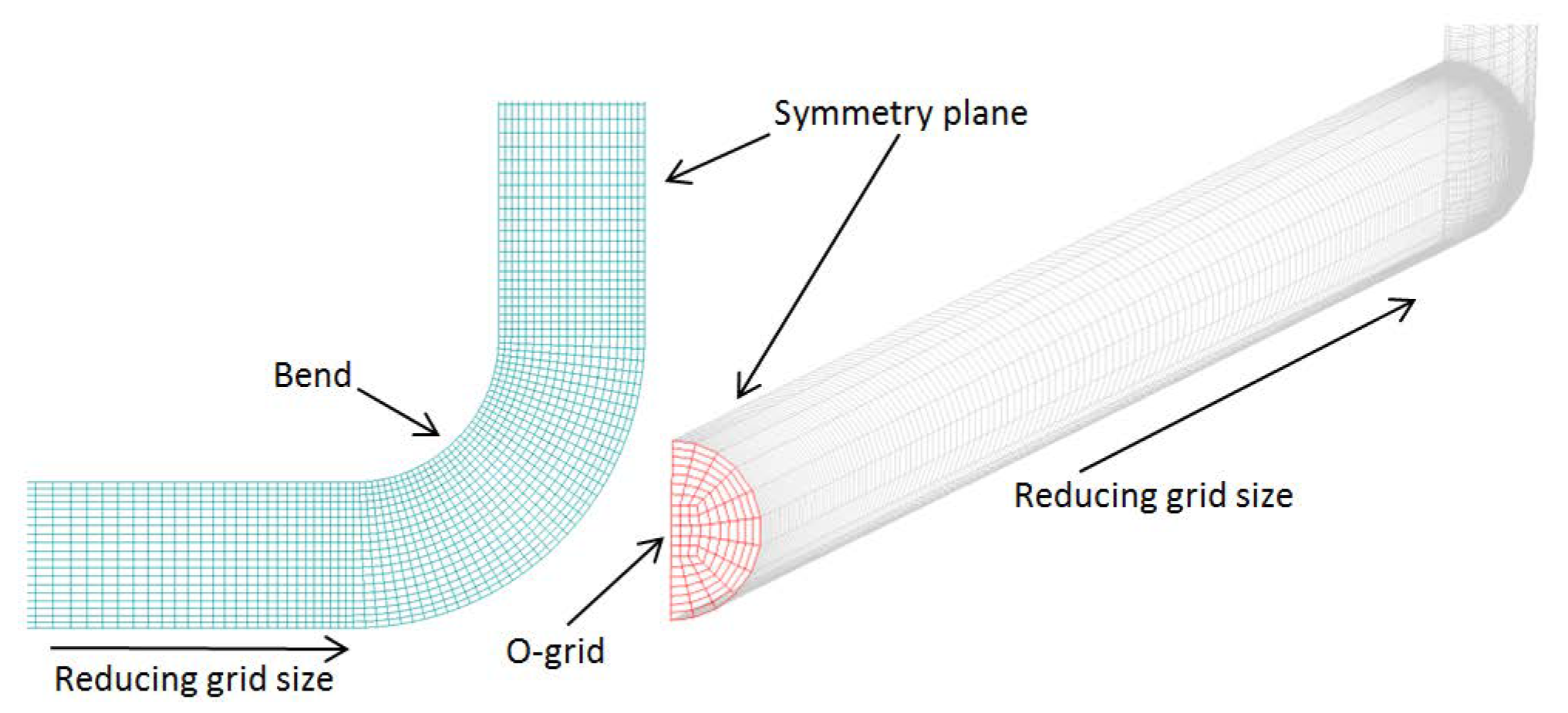
Figure 4 shows a part of the mesh corresponding to the lower horizontal section and a 90 upward bend of the set-up shown in Figure 3.
The outflow boundary has a stress-free outflow condition, which ensures zero diffusion flux on the outflow boundary. This is helpful in this case as the velocity and pressure conditions at the boundary are not known a priori.
The inflow boundary was provided with a constant axial flow velocity corresponding to the experimental average flow velocity. To add the effect of turbulence, ANSYS FLUENT provides the option of specifying an inflow turbulence intensity and hydraulic diameter, to calculate the values of and (see ANSYS [24] for details). In each case considered, the hydraulic diameter is equal to the pipe’s inner diameter as the pipes are circular. The inflow turbulence intensity is not known a priori in any of the experimental cases. However, for wall-bounded flows, the shear layers generate more turbulence than the inflow boundary alone, making the results insensitive to the inflow specifications (ANSYS [24]; this was also checked by varying the inflow turbulence intensity). However, to play safe, the inflow turbulence was restricted to and an ample distance from the inflow boundary was considered before accepting the flow as fully-developed.
Finally, as the wall boundary is treated with a wall function, the boundary conditions for and are calculated as per the wall function approach, instead of being set to 0 at the wall (can only be done if the entire wall region is refined). At the wall boundary, is thus set equal to the turbulence kinetic energy at the first grid point, obtained using the rationale defined by Launder and Spalding (see Launder and Spalding [5] for details).
4. Sensitivity Analysis
This section describes the analysis of the sensitivity of and to various rheological inputs and flow conditions. For each Herschel–Bulkley fluid mentioned in Table 1, a standard case of a long straight horizontal pipe was simulated for a range of flow velocities. The meshes were sized through the process described in Section 3.2 to ensure grid convergence. Here, the operational envelope is defined as the domain of rheological parameters and flow velocities (indirectly the ) within which, and when coupled with a RANS model, can accurately quantify the wall shear stress (hence, the pressure gradient) experienced by a pipe carrying the relevant Herschel–Bulkley fluid in turbulent flow.
This accuracy, in line with [4], is set at either an error, or an error, , as compared to the relevant experimental estimates. For completeness, an error of is also considered, to indicate that a numerical solution was obtained but inaccurate, in contrast with cases in which a converged numerical solution was not obtained.
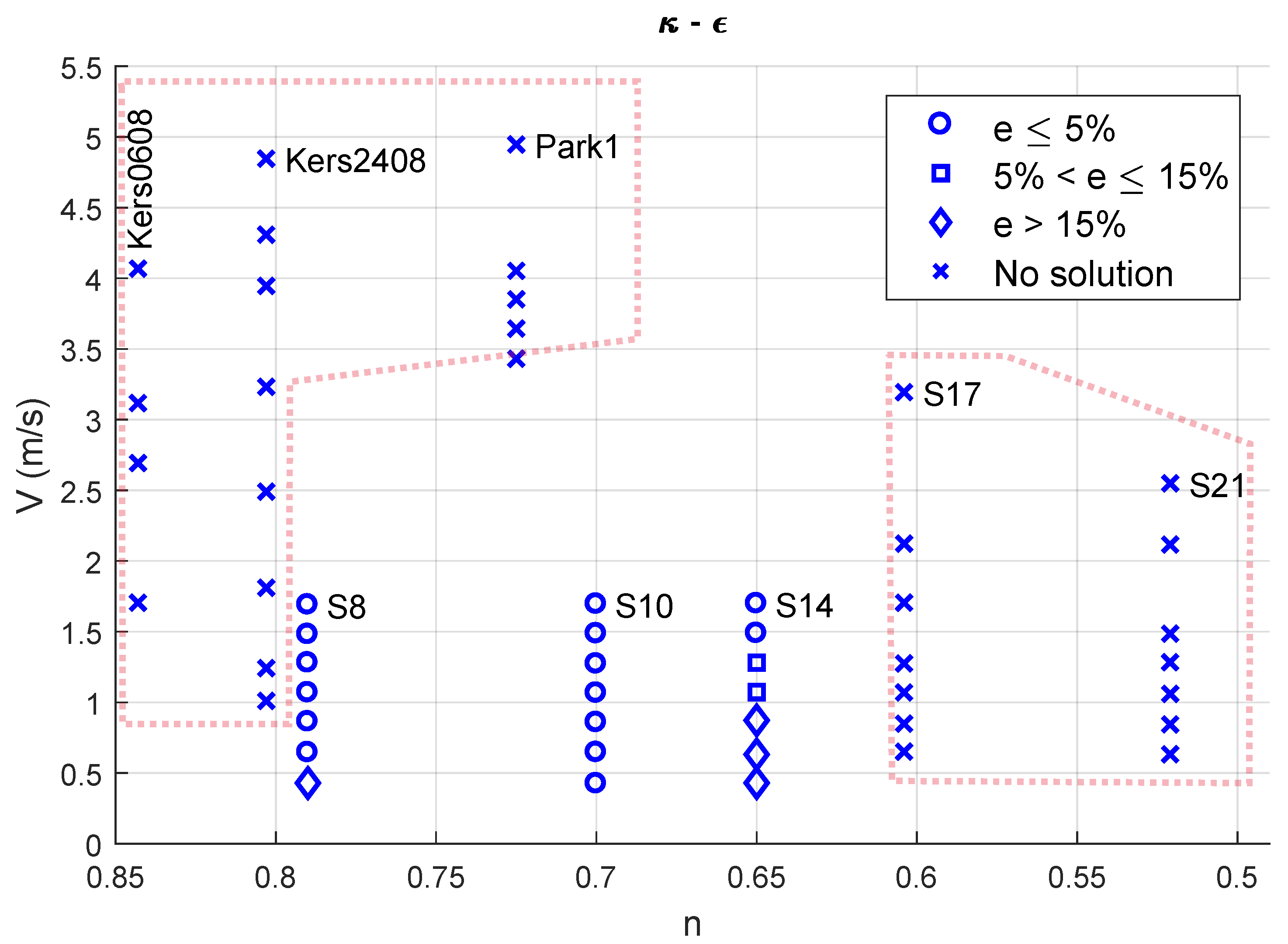
4.1. Flow Velocity, Behaviour Index and Accuracy
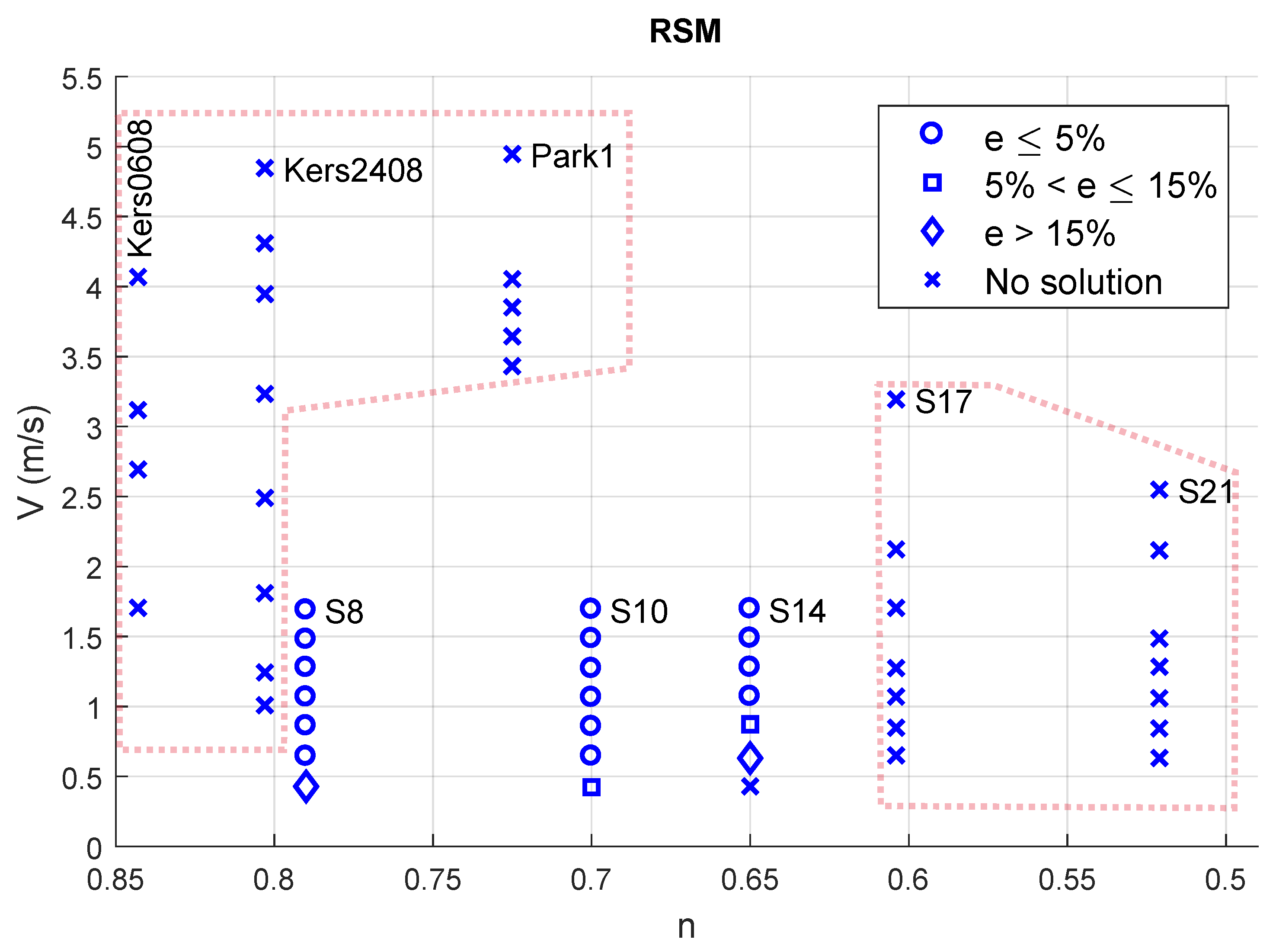
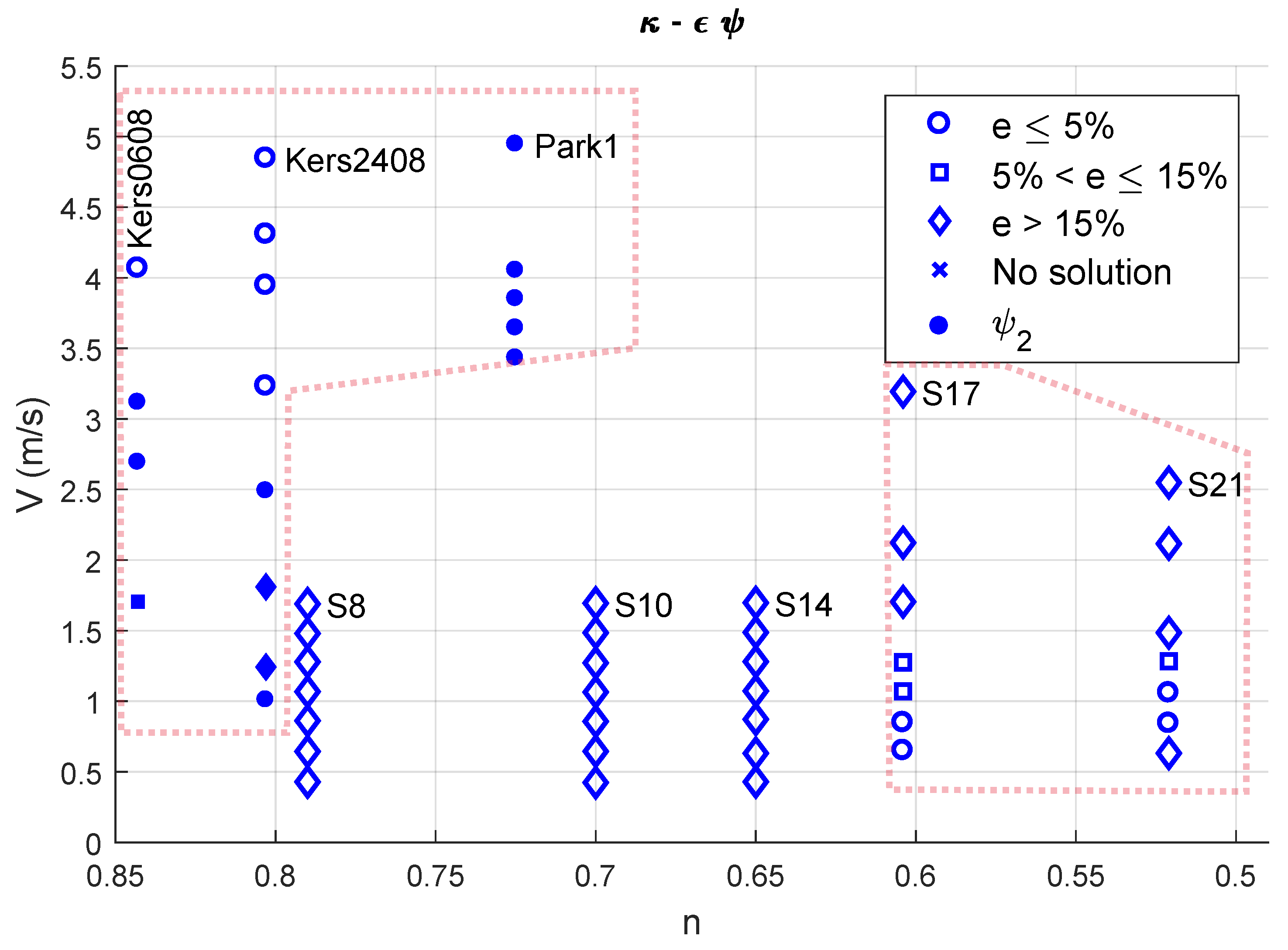
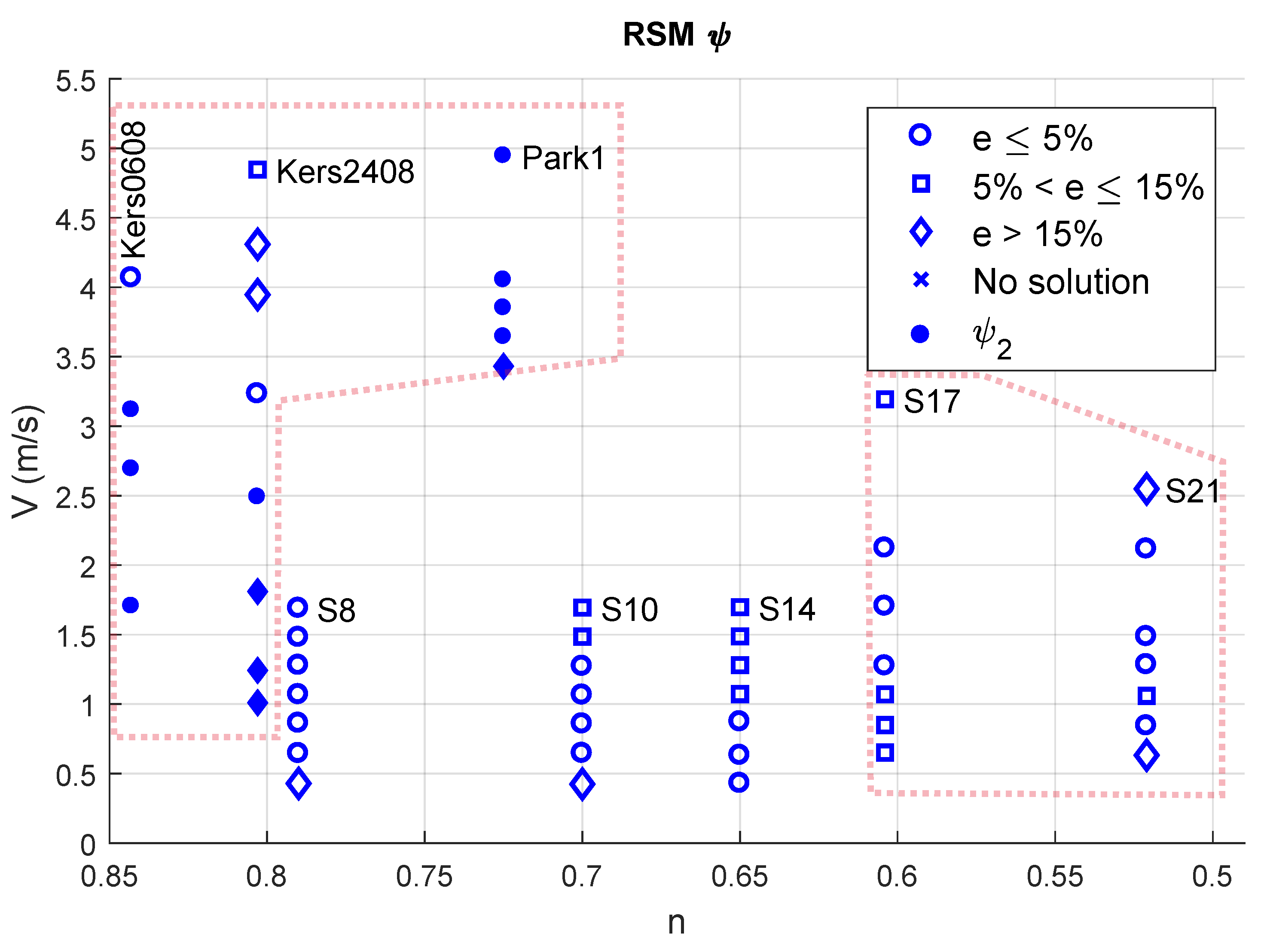
Figure 5, Figure 6, Figure 7 and Figure 8 show scatter plots of the relation between the flow velocity V, the behaviour index n and the accuracy achieved by various combinations of RANS models and wall functions. V is the average axial flow velocity inside the pipe; thus, the area-averaged axial velocity (henceforth referred to as the flow velocity, for simplicity). A ○ indicates , a □ and a ◇ . All values of e are the percentage difference between a numerical estimate and its experimental counterpart. Furthermore, for RANS models combined with or , all symbols (○, □ and ◇) correspond to , unless filled (or ●, ■ and ◆), in which case, they correspond to . A x represents no solution with either wall function.
Figure 5 and Figure 6 depict results obtained with the and RSM RANS models without or i.e., these cases used the standard Newtonian wall function proposed by Launder and Spalding [5] described in Section 3.1. One notices that no converged solution is obtained for the considered flow velocities, for slurries apart from , and . The region in which no solution is obtained is highlighted by dotted polygons in Figure 5, Figure 6, Figure 7 and Figure 8. Furthermore, the estimates for with either RANS model can only be considered accurate once V is more than 1 m/s (the aim is to transport the turbulent slurry with a flow velocity ranging from 0.5 m/s to 1.5 m/s). Apart from the lowest velocities considered, the wall shear stresses generated by and are well-estimated () by either RANS model (regions outside the dotted polygons).
Figure 7 and Figure 8 depict results obtained with the and RSM RANS models with or , the latter being shown with a filled (shaded) symbol. A stark difference between Figure 5, Figure 6, Figure 7 and Figure 8 is the existence of a converged numerical solution for slurries and the considered velocities, for which a solution was not obtained in the absence of and . These slurries are namely , , , and .
Comparing Figure 7 and Figure 8 in regard to and , there is no particular trend in the effect of the RANS model on the accuracy. However, a simple count reveals that, in most cases, RSM performs better than regarding the delivery of . Furthermore, given the low values of yield stress summarised in Table 1, none of these slurries require .
For , both RANS models deliver accurate results, with the lower velocities (when the shear stress is low enough) requiring the application of . As explained in [4] and shown in Figure 2, the reduction in flow velocity leads to a reduction in the wall shear stress; the ratio of the yield stress to the wall stress determines the extent of the plug-like unyielding region in the centre of the pipe, which also affects turbulent mixing. was proposed keeping this effect in mind and reducing the effective mixing length. Finally, numerical quantifications of are not only existent after the application of but also obtain an error , with either RANS model (except for the lowermost velocity when analysed with RSM). must be used in keeping with the relatively high yield stress of = 9.3 Pa.
A point worth noting is that, in contrast with the lower errors obtained during the analysis of , and with without or , using these wall functions leads to inaccurate solutions () for all velocities considered. However, the same is not noticed when these slurries are analysed with the RSM—in which case, the results are nearly the same, whereas remains the same with and without .
One may attribute this behaviour to the differences in the formulation of the two RANS models. The ignores anisotropy in the Reynolds-stress tensor, whereas the RSM incorporates all anisotropy by solving six transport equations for the different components of the Reynolds-stress tensor. Within the wall-bounded flow described here, the anisotropy arises primarily from the walls and the fact that the flow in the core converges onto an unyielding plug. However, the direct effect of these differences in formulation on the accuracy requires a more detailed analysis supported by experiments, which is beyond the scope of the research related to this article.
To facilitate the understanding of the observations mentioned above, it is necessary to incorporate the effect of the yield stress into the analysis. The yield stress is a property of the slurry; however, its ratio to the wall shear stress that is directly related to the flow velocity is consequential in governing the flow dynamics, to the extent of (or ) being essential for guaranteeing accurate estimates for Herschel–Bulkley slurries with acceptably high yield stresses. Therefore, the results from Figure 5, Figure 6, Figure 7 and Figure 8 are re-plotted while considering the ratio . Furthermore, given that the analysis so far is inconclusive as to the nature of the RANS model itself, the results will be segregated not in terms of the error but rather in terms of the RANS models for a fixed error.
4.2. Flow Velocity, Yield Stress and RANS Model
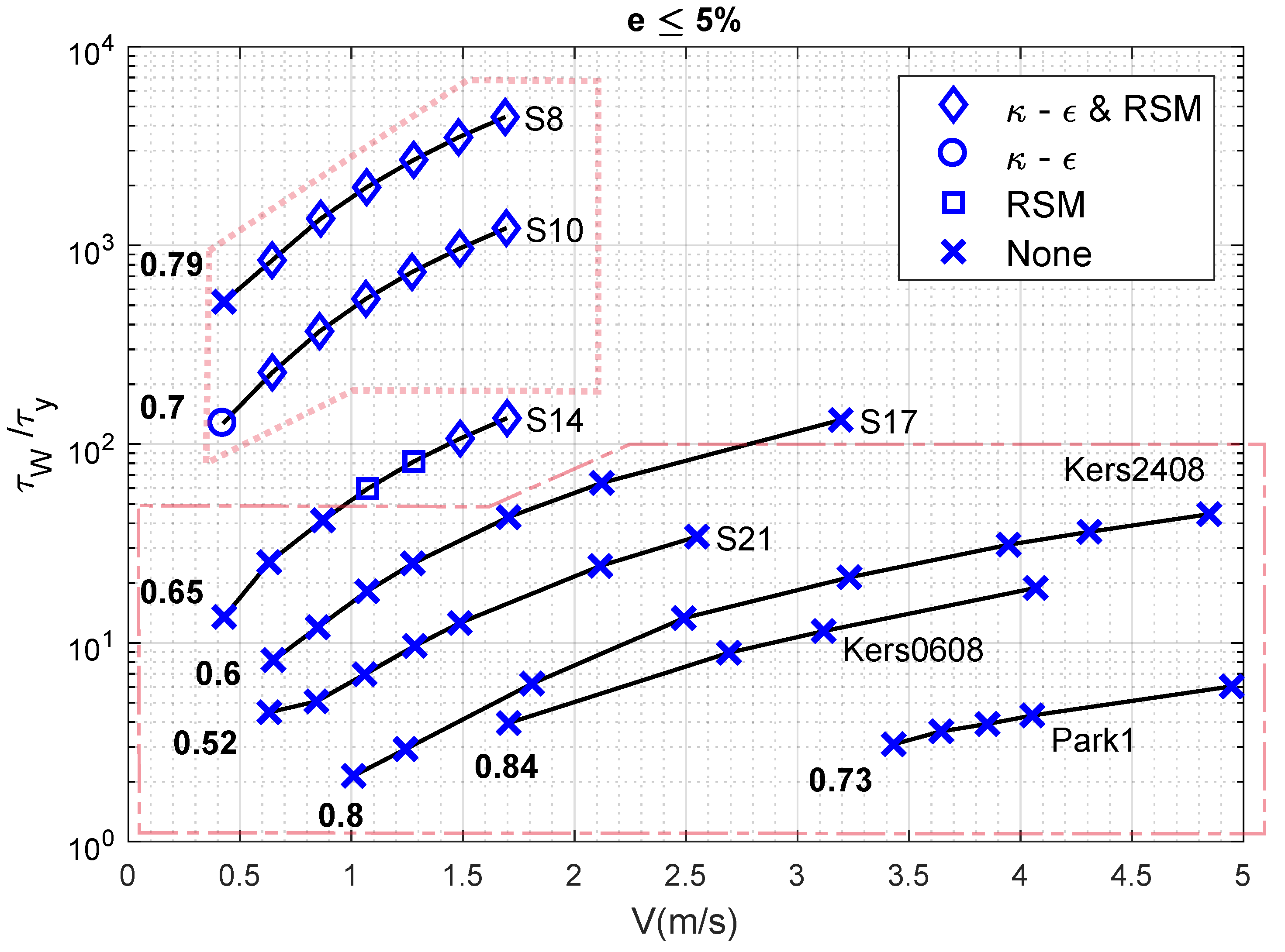
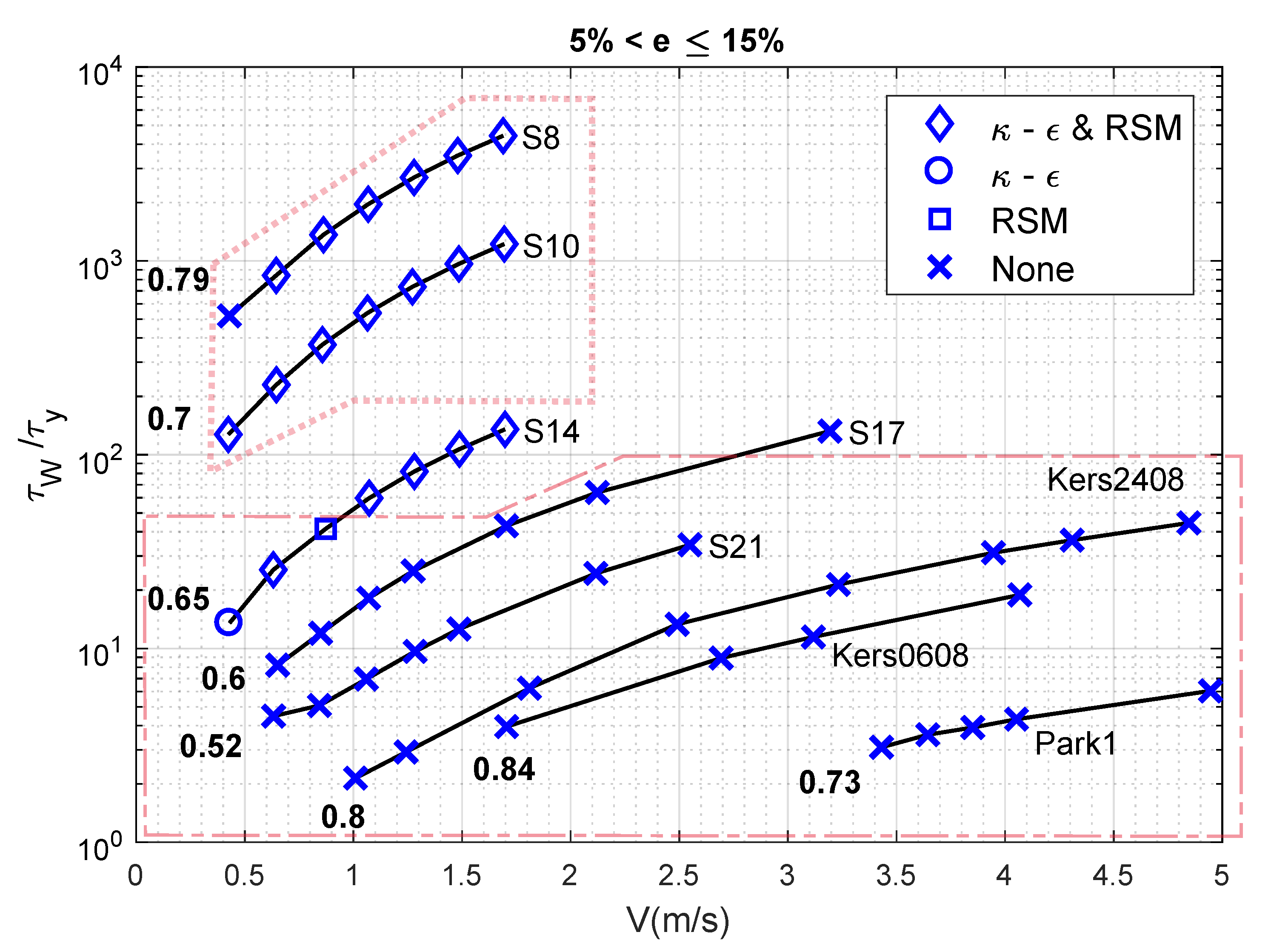
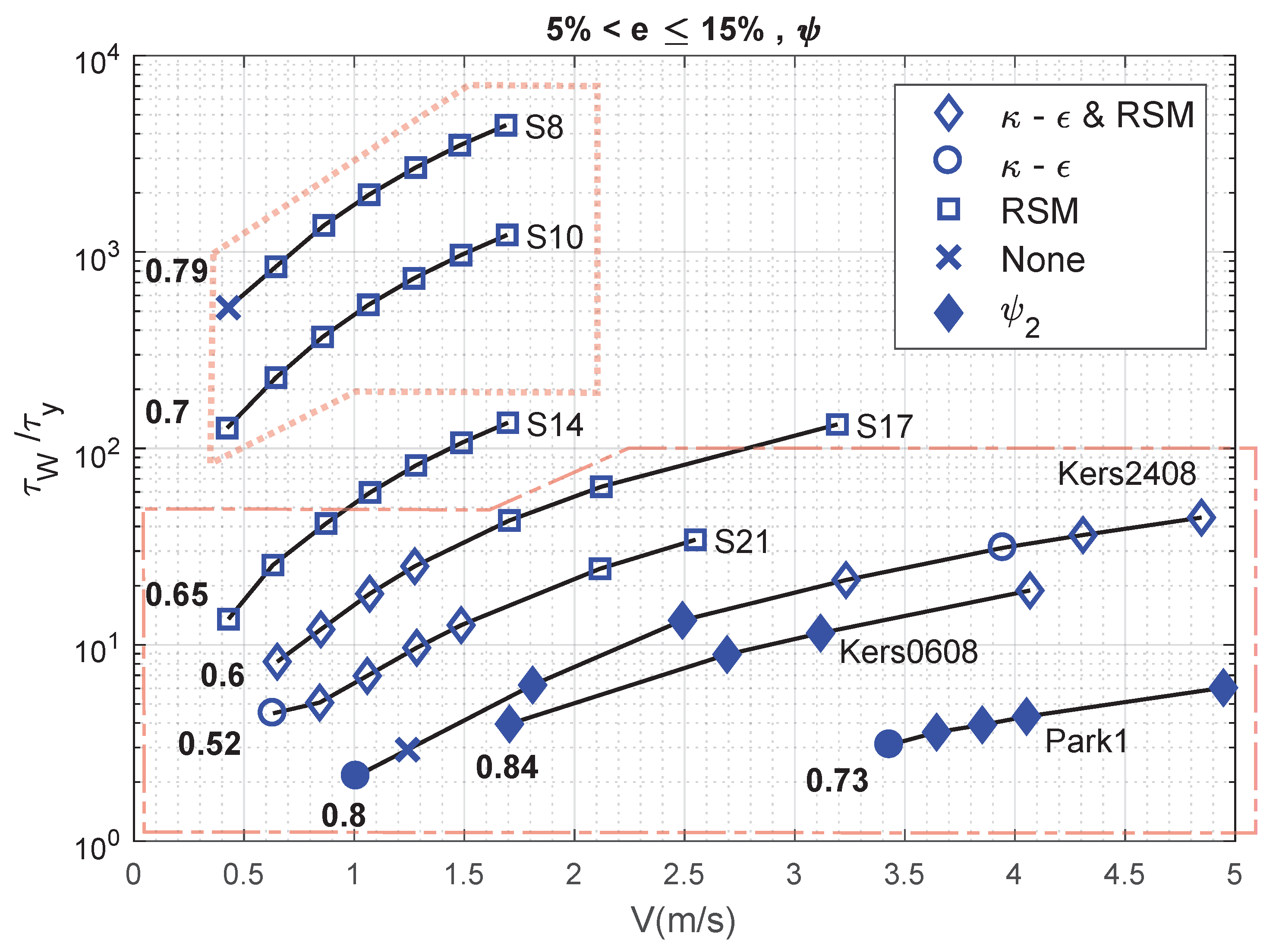
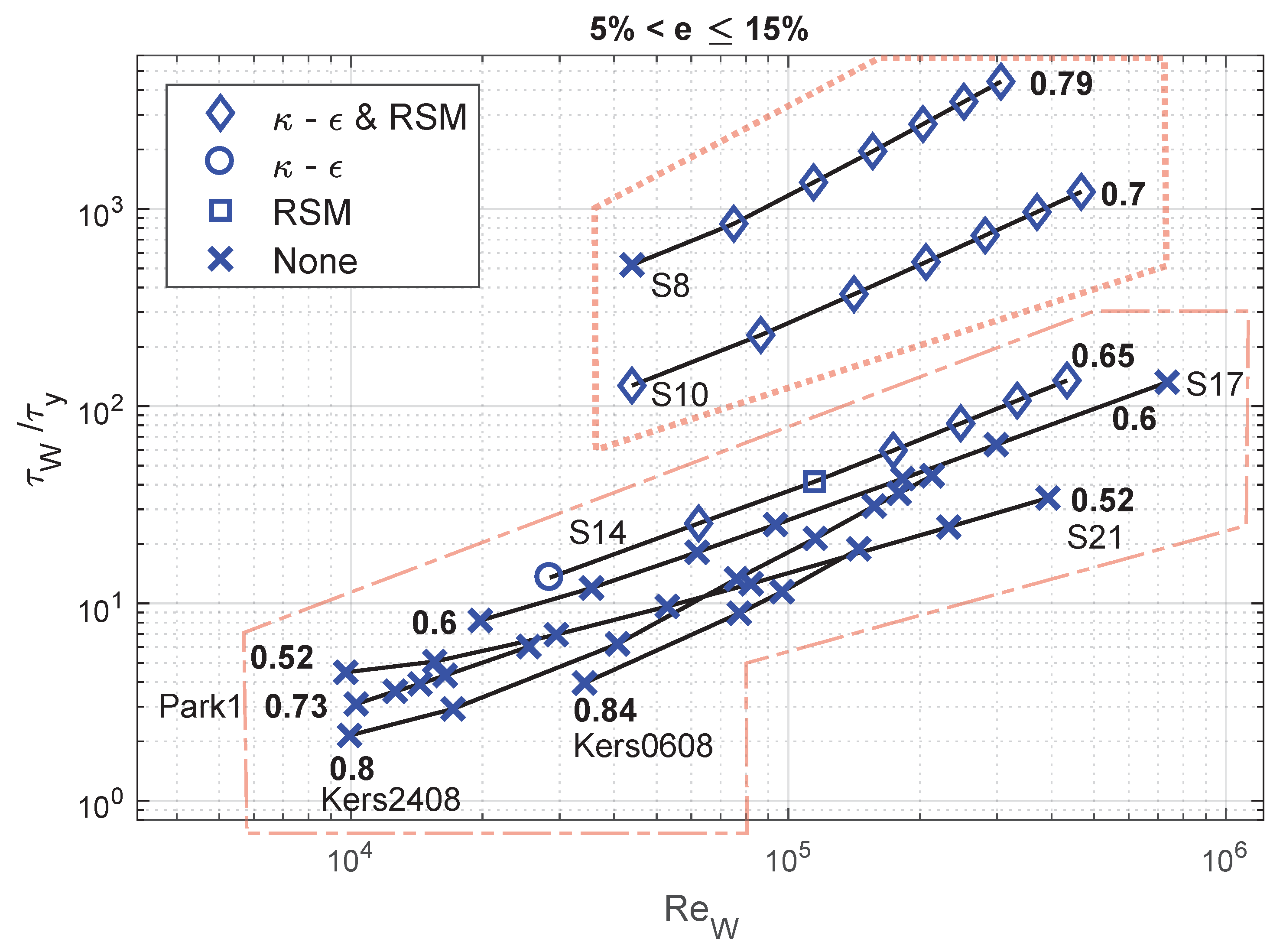
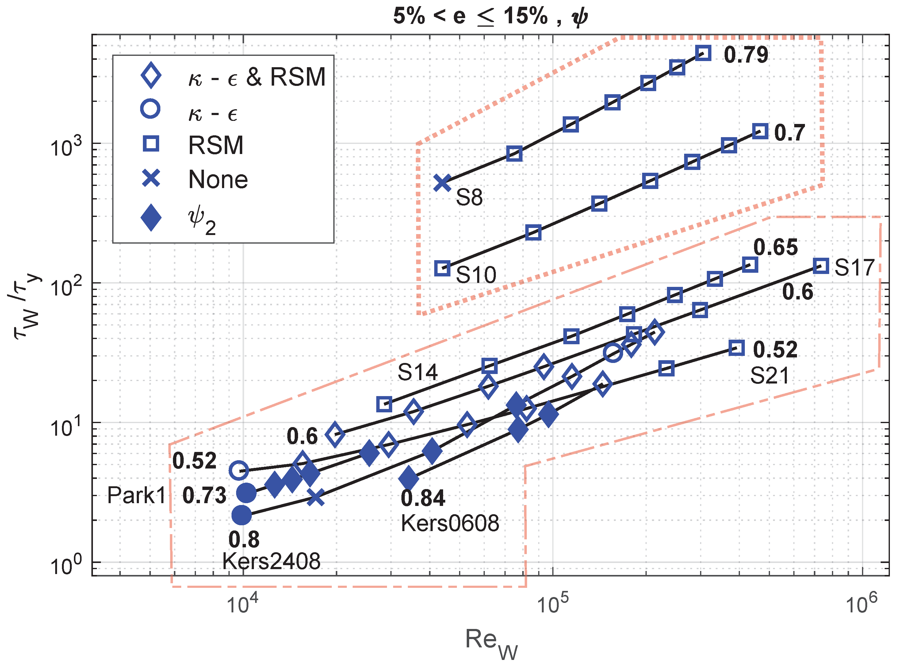
Figure 9, Figure 10, Figure 11 and Figure 12 plot the relationship between (logarithmic) and V, while relating them to the accuracy of the numerical simulation performed for those operating conditions, in terms of the RANS models used. Figure 9 and Figure 10 pertain to an error , whereas Figure 11 and Figure 12 pertain to an error ; out of these four plots, Figure 10 and Figure 12 represent solutions obtained with or , as indicated.
In all plots, namely Figure 9, Figure 10, Figure 11 and Figure 12, a ◇ means that both and RSM provided solutions within the error defined by the relevant plot ( in the case of Figure 9). Furthermore, a ○ indicates that only led to a solution within the mentioned error and a □ indicates that only the RSM led to a solution. A x means that none of the two RANS models led to a converged numerical solution or the error was beyond the value defined by the relevant plot. In Figure 10 and Figure 12, a filled symbol (●, ■ and ◆) represents .
A first look while comparing errors without or i.e., Figure 9 and Figure 11 against errors with or i.e., Figure 10 and Figure 12, reveals that the use of or is indeed necessary for a large number of experimental cases considered here. The approximate envelope within which this observation holds is indicated with a dashed polygon in Figure 9, Figure 10, Figure 11 and Figure 12. This observation is in line with those reported in Section 4.1. Only this time, one notices that and change a no solution (represented by a x) to a converged solution for test-cases with a ratio that is less than two orders of magnitude.
This trend is most apparent when is less than 20. Such a low ratio is attained when the rheological yield stress is high or when a slurry with a moderate to high yield stress flows with a small flow velocity, as suggested by Figure 9, Figure 10, Figure 11 and Figure 12. Furthermore, when the ratio is less than 10, more than one-tenth of the pipe’s radial extent is theoretically occupied by an unyielding region that does not promote turbulent mixing. This therefore requires the use of to obtain a numerically converged and accurate solution, as shown by shaded (filled) symbols in Figure 10 and Figure 12.
Another observation is that the above-mentioned trend of or promoting accuracy for very low values is valid across a range of behaviour indices, namely 0.52–0.84 in plots presented in this section. This range of behaviour index is sufficient to capture the change from a nearly Newtonian behaviour (0.84) towards a dominant non-Newtonian behaviour (0.52), as illustrated in the study on numerical model by Wilson and Thomas [37].
Furthermore, slurries with comparable behaviour indices but small to insignificant values of (, and in our case), do not require the combination of ( is no longer relevant as high enough for to be sufficient for accuracy) with a RANS model for an accurate numerical estimate. In fact, the standard or the RSM (as shown by ◇) are sufficient to guarantee an error .
The use of or requires a more involved discussion. Consider Figure 9 and Figure 10 for ; the values are between 10 are 100. The use of changes a no solution to for the lower velocities ( m/s) that concern a close to 10. On the other hand, for itself, the use of leads to a no solution for higher velocities ( m/s) for which, is more than 60. Thus, for a given rheology, the value of is perhaps consequential in determining whether must be used or not.
Furthermore, for slurries and with between 100 and 1000, the use of actually leads to a reduction in the performance of the model. Comparing Figure 9, Figure 10, Figure 11 and Figure 12, one notices that both and RSM lead to accurate quantifications, whereas the use of only provides an accurate estimate with the RSM. This is indicated by the change of most data points for and , from ◇ to □ within the dotted polygon.
Finally, comparing the plots in terms of the errors margins set for them i.e., for Figure 9 and Figure 10 and for Figure 11 and Figure 12, one observes that most x (no solution) change to a solution obtained with either RANS models. In addition, solutions obtained with either (○) or RSM (□) are obtainable with both models (◇) once the error margin is increased to .
4.3. Reynolds Number, Yield Stress and RANS Model
The analyses in Section 4.1 and Section 4.2 did not incorporate the consistency index m. In effect, the consistency index could be thought of as representing the Newtonian viscous aspects of a fluid, with the behaviour index n and the yield stress , contributing to any deviation from Newtonian behaviour.
However, as per Equations (8) and (9), the wall effective viscosity is directly related to the power of m, which influences the Reynolds number directly. Furthermore, the analysis from Section 4.2 considers various slurries at different velocities. Therefore, it is only sensible to observe the data from the analysis linking the yield stress and the flow velocity, in terms of vs. plots; as shown in Figure 13, Figure 14, Figure 15 and Figure 16. These are identical to the plots shown in Section 4.2 (Figure 9, Figure 10, Figure 11 and Figure 12) but with as the x-axis instead of the flow velocity V.
One notices that the experimental data used for the analysis spans a considerable range of Reynolds numbers i.e., . The region of interest in the previous section i.e., , also spans the mentioned range of Reynolds numbers. Furthermore, it is worth mentioning that this region also includes a range of behaviour indices i.e., 0.52–0.84.
Therefore, combining the analysis from Section 4.2 and Figure 13, Figure 14, Figure 15 and Figure 16, the observation that (or as the need may be) leads to more accurate numerical estimates with RANS models when the flow conditions are such that , is valid not only for a range of Reynolds numbers but also an acceptable range of consistency indices.
This helps establish that, within an envelope defined by and , the use of the proposed wall function (or when is very low i.e., less than 10) is necessary for accuracy, shown as the dashed polygon in Figure 13, Figure 14, Figure 15 and Figure 16 and corresponding with the same region in Figure 9, Figure 10, Figure 11 and Figure 12. Furthermore, outside of this envelope in terms of , the use of is not required and may perhaps lead to a loss in accuracy or compromise the functioning of the model, in our case, shown as the dotted polygon in Figure 9, Figure 10, Figure 11 and Figure 12. At the moment, it is not possible to provide a clear and complete explanation as to why the use of with an RSM for a test-case in which still leads to accurate estimates with the RSM but not with the model. This may simply be because of differences in the models’ formulations [38] or mathematical artefact, either of which is beyond the scope of this article, as suggested previously.
5. Conclusions
Based on the mentioned observations, one may conclude that the proposed wall functions and when combined with the standard or RSM could lead to accurate numerical quantification of the wall shear experienced by a circular pipe carrying a Herschel–Bulkley fluid in turbulent flow. However, the ability of this numerical method (RANS combined with or ) to be accurate is limited by an operational envelope.
Simulations of test-cases that vary in Reynolds number ( based on the wall effective viscosity) within , while covering a range of behaviour indices 0.52 to 0.84, indicate that the operational envelope is determined by the ratio of the wall shear stress to the rheological yield stress of the Herschel–Bulkley fluid in question i.e., . For values of below 100, the use of with a RANS model generates an accurate () estimate of the wall shear stress, which otherwise is not possible with the standard Newtonian wall function [5]. Furthermore, as one approaches values below 10, must be used with to account for a stronger Herschel–Bulkley behaviour.
On the other hand, for values of greater than 100 (and all the way up to as tested here), both the and RSM combined with the standard Newtonian wall function achieve an accuracy of . The use of leads to a faulty solution ( or not converged) with the model but not with the RSM. This may be attributed to fundamental differences between the formulations of the two RANS models; further investigation in this regard is required.
In relation with concentrated domestic slurry, CFD is a promising tool to analyse turbulent slurry flows (Herschel–Bulkley type), while using the proposed operational envelope as a guideline. The pressure drop as estimated through CFD can be used to size the pumps required for the transport of concentrated domestic slurry. Further experimentation and numerical simulations could provide more insight into the nature of turbulence in such flows, which could in turn be used to develop (or modify existing) simpler engineering models. With such models, one could obtain the frictional losses through an entire urban sewer system transporting concentrated domestic slurry. Finally, the use of () need not be restricted to the transport of slurry. Being generalised functions, they could be used to simulate any system carrying a Herschel–Bulkley fluid in turbulent flow.
Author Contributions
D.M. conducted the numerical simulations, whereas A.K.T.R. conducted the experiments for S8, S10, S14, S17 and S21. Both D.M. and A.K.T.R. were supervised by J.v.L. and F.C.
Funding
This article is a result of the research carried out at the Delft University of Technology, Delft and funded under the grant agreement 13347 by NWO-domain TTW, Foundation Deltares, Stowa, Foundation RIONED, Waternet, Waterboard Zuiderzeeland, Grontmij and XYLEM. We acknowledge the support of the funding bodies and their contributions to this research.
Conflicts of Interest
The authors declare no conflict of interest.
Abbreviations
The following abbreviations are used in this manuscript:
| NS | Navier-Stokes |
| CFD | Computational fluid dynamics |
| RANS | Reynolds-averaged Navier-Stokes |
| RSM | Reynolds stress model |
| SIMPLE | Semi-implicit method for pressure-linked equations |
| NWO | Nederlandse Organisatie voor Wetenschappelijk Onderzoek |
| TTW | Toegepaste en Technische Wetenschappen |
References
- Thota Radhakrishnan, A.; van Lier, J.; Clemens, F. Rheological characterisation of concentrated domestic slurry. Water Res. 2018, 141, 235–250. [Google Scholar] [CrossRef]
- Thota Radhakrishnan, A.K.; van Lier, J.; Clemens, F. Rheology of Un-Sieved Concentrated Domestic Slurry: A Wide Gap Approach. Water 2018, 10, 1287. [Google Scholar] [CrossRef]
- Chabbra, R.P.; Richardson, J.F. Non-Newtonian Flow in the Process Industries, 1st ed.; Butterworth-Heinemann: Oxford, UK, 1999. [Google Scholar]
- Mehta, D.; Thota-Radhakrishnan, A.K.; van Lier, J.; Clemens, F. A wall boundary condition for the simulation of a turbulent non-Newtonian domestic slurry in pipes. Water 2018, 10, 124. [Google Scholar] [CrossRef]
- Launder, B.E.; Spalding, D.B. The numerical computation of turbulent flows. Comput. Methods Appl. Mech. Eng. 1974, 3, 269–289. [Google Scholar] [CrossRef]
- Herschel, W.H.; Bulkley, R. Konsistenzmessungen von Gummi-Benzollösungen. Kolloid-Zeitschrift 1926, 39, 291–300. [Google Scholar] [CrossRef]
- Oldroyd, J.G. A rational formulation of the equations of plastic flow for a Bingham solid. Math. Proc. Camb. Philos. Soc. 1947, 43, 100–105. [Google Scholar] [CrossRef]
- Skelland, A.H.P. Non-Newtonian Flow and Heat Transfer; John Wiley & Sons: Hoboken, NJ, USA, 1967. [Google Scholar]
- Govier, G.W.; Aziz, K. The Flow of Complex Mixtures in Pipes; R.E. Krieger Pub. Co.: New York, NY, USA, 1972. [Google Scholar]
- Bird, R.B.; Dai, G.C.; Yarusso, B.J. The rheology and flow of viscoplastic materials. Rev. Chem. Eng. 1983, 1, 1–70. [Google Scholar] [CrossRef]
- Bird, R.B.; Armstrong, R.C.; Hassager, O. Dynamics of Polymeric Liquids, Vol. 1: Fluid Mechanics, 2nd ed.; John Wiley & Sons: New York, NY, USA, 1987. [Google Scholar]
- Heywood, N.I.; Cheng, D.C.H. Comparison of methods for predicting head loss in turbulent pipe flow of non-Newtonian fluids. Trans. Inst. Meas. Control 1984, 6, 33–45. [Google Scholar] [CrossRef]
- Torrance, B.M. Friction factors for turbulent non-Newtonian fluid flow in circular pipes. S. Afr. Mech. Eng. 1963, 13, 89–91. [Google Scholar]
- Hanks, R.W. Low Reynolds number turbulent pipeline flow of pseudohomogeneous slurries. In Proceedings of the Hydrotransport 5 Conference, Hanover, Germany, 8–11 May 1978; pp. 8–11. [Google Scholar]
- Ferziger, J.; Perić, M. Computational Methods for Fluid Dynamics, 3rd ed.; Springer Science and Business Media: New York, NY, USA, 2012. [Google Scholar]
- Davidson, P.A. Turbulence—An Introduction for Scientists and Engineers; Oxford University Press: Oxford, UK, 2004. [Google Scholar]
- Schlichting, H. Boundary-Layer Theory, 8th ed.; Springer: New York, NY, USA, 2017. [Google Scholar]
- Prandtl, L. Zur turbulenten Strömung in glatten Röhren. Z. Angew. Math. Mech. 1925, 5, 136–139. [Google Scholar]
- Prandtl, L. Neure Ergebnisse der Turbulenzforschung. Z. Ver. Deutsch. Ingenieure 1933, 77, 105–114. [Google Scholar]
- von Kármán, T. Mechanische Ähnlichkeit und Turbulenz; Sonderdrucke aus den Nachrichten von der Gesellschaft der Wissenschaften zu Göttingen: Mathematisch-physische Klasse; Weidmannsche Buchh: Berlin, Germany, 1930. [Google Scholar]
- Rudman, M.; Blackburn, H.M. Direct numerical simulation of turbulent non-Newtonian flow using a spectral element method. App. Math. Model. 2006, 30, 1229–1248. [Google Scholar] [CrossRef]
- Slatter, P.T. Transitional and Turbulent Flow of Non-Newtonian Slurries in Pipes. Ph.D. Thesis, University of Cape Town, Cape Town, South Africa, 1995. [Google Scholar]
- Park, J.T.; Mannheimer, R.J.; Grimley, T.A.; Morrow, T.B. Pipe flow measurements of a transparent non-Newtonian slurry. J. Fluids Eng. 1989, 111, 331–336. [Google Scholar] [CrossRef]
- ANSYS. ANSYS FLUENT User’s Guide; Ansys Inc.: Canonsburg, PA, USA, 2011. [Google Scholar]
- Rudman, M.; Blackburn, H.M.; Graham, L.J.W.; Pullum, L. Turbulent pipe flow of shear-thinning fluids. J. Non-Newton. Fluid Mech. 2004, 118, 33–48. [Google Scholar] [CrossRef]
- Malin, M.R. The turbulent flow of Bingham plastic fluids in smooth circular tubes. Int. Commun. Heat Mass Transf. 1997, 24, 793–804. [Google Scholar] [CrossRef]
- Malin, M.R. Turbulent pipe flow of Herschel-Bulkley fluids. Int. Commun. Heat Mass Transf. 1998, 25, 321–330. [Google Scholar] [CrossRef]
- Bartosik, A.S. Modification of κ-ϵ model for slurry flow with yield stress. In Proceedings of the 10th International Conference on Numerical Methods in Laminar and Turbulent Flows, Swansea, UK, 21–25 July 1997; Volume 10, pp. 265–274. [Google Scholar]
- Bartosik, A.S. Modelling of a turbulent flow using the Herschel-Bulkley rheological model. Chem. Process Eng. Inzynieria Chem. Proces. 2006, 27, 623–632. [Google Scholar]
- Tanner, R.I.; Milthorpe, J.H. Numerical simulation of the flow of fluids with yield stress. In Numerical Methods in Laminar and Turbulent Flow, Proceedings of the Third International Conference, Seattle, WA, 8–11 August 1983; Pineridge Press: Swansea, UK, 1983. [Google Scholar]
- Mitsoulis, E. Flows of Viscoplastic Materials: Models and Computations; Rheology Reviews, British Society of Rheology: London, UK, 2007; pp. 135–178. [Google Scholar]
- Metzner, A.B.; Reed, J.C. Flow of non-Newtonian fluids—Correlation of the laminar, transition and turbulent-flow regions. AIChE J. 1955, 1, 434–440. [Google Scholar] [CrossRef]
- Dean, W. XVI. Note on the motion of fluid in a curved pipe. Lond. Edinb. Dublin Philos. Mag. J. Sci. 1927, 4, 208–223. [Google Scholar] [CrossRef]
- Tunstall, M.J.; Harvey, J.K. On the effect of a sharp bend in a fully developed turbulent pipe-flow. J. Fluid Mech. 1968, 34, 595–608. [Google Scholar] [CrossRef]
- Rütten, F.; Schröder, W.; Meinke, M. Large-eddy simulation of low frequency oscillations of the Dean vortices in turbulent pipe bend flows. Phys. Fluids 2005, 17, 035107. [Google Scholar] [CrossRef]
- Kalpakli, A.; Örlü, R. Turbulent pipe flow downstream a 90° pipe bend with and without superimposed swirl. Int. J. Heat Fluid Flow 2013, 41, 103–111. [Google Scholar] [CrossRef]
- Wilson, K.C.; Thomas, A.D. A new analysis of the turbulent flow of non-Newtonian fluids. Can. J. Chem. Eng. 1985, 63, 539–546. [Google Scholar] [CrossRef]
- Wilcox, D.C. Turbulence Modeling in CFD, 3rd ed.; DCW Industries: La Canada Flintridge, CA, USA, 2006. [Google Scholar]
Figure 1.
A schematic of a circular horizontal pipe [4].
Figure 1.
A schematic of a circular horizontal pipe [4].

Figure 2.
The effective mixing region in a pipe carrying an Herschel–Bulkley fluid with yield stress . The unyielding plug represents the region wherein .
Figure 2.
The effective mixing region in a pipe carrying an Herschel–Bulkley fluid with yield stress . The unyielding plug represents the region wherein .

Figure 3.
A schematic of a part of the experimental set-up showing the location of the pressure sensors used for validation [1,2] (Courtesy: Stichting Deltares).

Figure 4.
The computational grid for the experimental set-up. The cross section is an O-grid, even across the bend.
Figure 4.
The computational grid for the experimental set-up. The cross section is an O-grid, even across the bend.

Figure 5.
Error with the standard model without (or ).

Figure 6.
Error with the standard RSM without (or ).

Figure 7.
Error with the model with (or , filled symbols).

Figure 8.
Error with the RSM with (or , filled symbols).

Figure 9.
Performance of the standard RANS models to achieve an error .

Figure 10.
Performance of the standard RANS models combined with to achieve an error .

Figure 11.
Performance of the standard RANS models to achieve an error .

Figure 12.
Performance of the standard RANS models combined with to achieve an error .

Figure 13.
Performance of the standard RANS models to achieve an error .

Figure 14.
Performance of the standard RANS models combined with to achieve an error .

Figure 15.
Performance of the standard RANS models to achieve an error .

Figure 16.
Performance of the standard RANS models combined with to achieve an error .


Table 1.
The test-cases considered for this article. The first two are from Slatter [22], from Park et al. [23] and the last five belong to experimental data supplied by the co-authors [1,2].
| Case | (kg/m) | (Pa) | m (Pas) | n | D (m) | Reference | |
|---|---|---|---|---|---|---|---|
| KERS2408 | 1061 | 1.04 | 0.0136 | 0.8031 | 0.079 | 380 | Slatter [22] |
| KERS0608 | 1071 | 1.88 | 0.0102 | 0.8428 | 0.079 | 380 | Slatter [22] |
| PARK1 | 1012 | 9.30 | 0.0894 | 0.7254 | 0.051 | 590 | Park et al. [23] |
| S8 | 1052 | 0.0014 | 0.0041 | 0.7900 | 0.100 | 450 | Thota Radhakrishnan et al. [1] |
| S10 | 1068 | 0.0052 | 0.0071 | 0.7000 | 0.100 | 450 | Thota Radhakrishnan et al. [1] |
| S14 | 1091 | 0.0490 | 0.0124 | 0.6500 | 0.100 | 450 | Thota Radhakrishnan et al. [1] |
| S17 | 1113 | 0.1585 | 0.0328 | 0.6043 | 0.100 | 450 | Thota Radhakrishnan et al. [1] |
| S21 | 1146 | 0.4316 | 0.0831 | 0.5207 | 0.100 | 450 | Thota Radhakrishnan et al. [1] |
© 2018 by the authors. Licensee MDPI, Basel, Switzerland. This article is an open access article distributed under the terms and conditions of the Creative Commons Attribution (CC BY) license (http://creativecommons.org/licenses/by/4.0/).
Share and Cite
MDPI and ACS Style
Mehta, D.; Thota Radhakrishnan, A.K.; Van Lier, J.; Clemens, F. Sensitivity Analysis of a Wall Boundary Condition for the Turbulent Pipe Flow of Herschel–Bulkley Fluids. Water 2019, 11, 19. https://doi.org/10.3390/w11010019
AMA Style
Mehta D, Thota Radhakrishnan AK, Van Lier J, Clemens F. Sensitivity Analysis of a Wall Boundary Condition for the Turbulent Pipe Flow of Herschel–Bulkley Fluids. Water. 2019; 11(1):19. https://doi.org/10.3390/w11010019
Chicago/Turabian StyleMehta, Dhruv, Adithya Krishnan Thota Radhakrishnan, Jules Van Lier, and Francois Clemens. 2019. "Sensitivity Analysis of a Wall Boundary Condition for the Turbulent Pipe Flow of Herschel–Bulkley Fluids" Water 11, no. 1: 19. https://doi.org/10.3390/w11010019
Note that from the first issue of 2016, this journal uses article numbers instead of page numbers. See further details here.