Numerical Simulation of Hydraulic Jumps. Part 1: Experimental Data for Modelling Performance Assessment


1
Hydraulic Engineering Section, Aachen University of Applied Sciences, Bayernallee 9, 52066 Aachen, Germany
2
Hydraulics in Environmental and Civil Engineering, University of Liège, Chemin des Chevreuils, 1, B52/3, Liège 4000, Belgium
3
Department of Civil, Architectural and Environmental Engineering, University of Naples Federico II, Via Claudio 21, 80125 Napoli, Italy
*
Author to whom correspondence should be addressed.
Water 2019, 11(1), 36; https://doi.org/10.3390/w11010036
Submission received: 31 October 2018
/
Revised: 19 December 2018
/
Accepted: 20 December 2018
/
Published: 25 December 2018
(This article belongs to the Section Hydraulics and Hydrodynamics)
Abstract
:Hydraulic jumps have been the object of extensive experimental investigation, providing the numerical community with a complete case study for models’ performance assessment. This study constitutes an exhaustive literature review on hydraulic jumps’ experimental datasets. Both mean and turbulent parameters characterising hydraulic jumps are comprehensively discussed, presenting at least a reference to one dataset. Three studies stand out over other datasets due to their completeness. Using them as reference for model validation may ensure homogeneous and comparable performance assessment for the upcoming numerical models. Experimental inaccuracies are also addressed, allowing the numerical modeller to understand the uncertainties of reduced physical models and its limitations. Part 2 presents the three-dimensional numerical investigations to date and their main achievements.
1. Introduction
Hydraulic jumps have been largely studied due to their relevance in hydraulic engineering applications [1,2,3]. When a hydraulic jump takes place, supercritical high velocity (oftentimes aerated) flows abruptly slow down, leading to a subcritical flow, which benefits structural stability and safe hydraulic conditions for river environments. This rapidly varied flow holds a considerable relevance also in environmental hydraulics, as it leads to strong reoxygenation ratios, and in eco-hydraulics where unprecedented hyporheic paths in river flows appear due to the occurring dynamic pressures [4,5]. Hence, the hydraulic jump is a phenomenon undergoing continuous research. Certainly, energy dissipation is its most distinctive feature in hydraulic engineering applications. Energy dissipation is one of the key aspects of hydraulic engineering, either as a continuous or as a sudden flow phenomenon. When high quantities of kinetic energy are expected in flows over hydraulic structures, an energy dissipator must be conveniently designed to safely dissipate the excess of energy. It must be noted that the excess of energy during extreme events can surpass many times the energy produced in a nuclear power plant [6]. Hence, the role of the stilling basin becomes critical and both its hydraulic and structural performance must be secured.
The canonical case of energy dissipator is the hydraulic jump (Figure 1), whose description dates back to Leonardo Da Vinci [2]. With the studies of Bidone in 1820 [7,8] and Bélanger in 1828 [9,10] and 1841 [10,11], first experimental and analytical steps were undertaken. Most relevant studies were built upon the solid ground set by the experimental study of Bakhmeteff and Matzke [12], the first turbulence estimations in hydraulic jumps of Rouse et al. [13], the wall jet analogy of Rajaratnam [14] and the turbulence structure study of Resch and Leutheusser [15]. Most detailed air–water flow turbulent features of hydraulic jumps started to be systematically reported after Chanson and Brattberg [16] and an up-to-date compendium of turbulent scales in hydraulic jumps can be found in Wang and Murzyn [17].
Research has also been conducted on non-conventional hydraulic jumps since the study of Warnock [18], covering hydraulic jumps over rough surfaces [19,20,21] to hydraulic jumps over methodologically disposed blocks and sills. Standardized complex designs became popular after the United States Bureau of Reclamation (USBR) guidelines of Peterka [22]—its first edition being released in 1958—and the Saint Anthony Falls (SAF) basin of Blaisdell [23]. A review of different types of basins can be found in Hager [2]. Nonetheless, research has not been that fruitful and knowledge on these types of basins is rather limited when compared to the canonical hydraulic jump counterpart (despite its obvious practical interest!).
As presented above, most advances have been accomplished through extensive experimental observation and some limited theoretical analyses. Nowadays, hydraulic jumps still represent one of the most active fields of research within the air–water flows hydraulic engineering community. With the emergence of cost-effective computer power given by the development of High Performance Computing techniques and hardware, some studies have been disclosed. Despite some relevant results, rigor is the object of dispute and some controversy has been raised by some authors concerning proper verification and validation [24,25]. The apparent lack of well-accepted numerical modelling guidelines may contribute to this issue, hence resulting in new studies sometimes lacking solid procedures, which puts their results continuously under dispute.
In Part 1 of this study, the most relevant features of the classic hydraulic jump are dissected in Section 2, briefly presenting the basic principles and providing some insight on the flow structure. Section 3 presents a brief discussion on the relevance of this type of flow, which represents a challenging flow in environmental fluid mechanics, whereas it converges a mature level of experimental research. Section 4 presents different common and new air–water flows instrumentations and the associated uncertainties and limitations. Conclusions are finally presented in Section 5. Part 1 of this study is intended to provide the numerical modeller, if unfamiliar with the experimental methodologies, with a deep insight on the available experimental datasets and their limitations. The reader is addressed to Part 2 [26] for an overview on three-dimensional numerical modelling techniques and current achievements on the hydraulic jump numerical modelling.
2. The Hydraulic Jump Case Study
2.1. General Remarks
When a high-speed supercritical flow meets a slower moving water flow, a hydraulic jump can take place. An exception can be found in the recent studies of Kabiri-Samani et al. [27] and Kabiri-Samani and Naderi [28], where supercritical flow transitions to subcritical without a hydraulic jump. A hydraulic jump takes place as a compatibility of momentum between upstream and downstream flow and it is often regarded as a standing wave. Similar types of flows can be found in propagating bores [29,30,31,32,33]. The case where the hydraulic jump takes place over a smooth horizontal rectangular channel is the well-known classic hydraulic jump (CHJ). It is the most widely documented type of hydraulic jump as it serves as a comparison for more complex cases, for instance: the hydraulic jump over arbitrary sections—or gradually varying width sections [3,34]—with different roughness surfaces and over inclined aprons or under submerged conditions [2].
For the CHJ, the most relevant variable is the sequent depth relationship. It can be described in terms of the inlet Froude number as [10]:
where d is the water depth and the subscripts 1 and 2 correspond to the upstream and downstream sections, respectively. Equation (1) is commonly known as the Bélanger equation. The Froude number for the inlet section of a CHJ can be defined as:
with the cross-section average velocity and g the gravity acceleration. The Froude number represents the balance between inertial and gravitational forces and takes values over unity for supercritical flows and below for subcritical flows. Definition for arbitrary cross-sectional channels can be found in literature [3,34].
Knowledge on the necessary sequent depths allows design of safe hydraulic structures and, additionally, enables computation of some other basic hydraulic jump properties, as, for instance, the dissipated energy. However, Equation (1) stands for a frictionless CHJ. Hager and Bremen [35] presented a modification which accounts for the smooth wall friction contribution. This implies a slight reduction in the conjugate depth relationship, as shown in Figure 2 and as discussed by Chanson [34] for hydraulic jumps over arbitrary cross-sections. An alternative approach contemplating hydraulic jumps over a rough bed can be found in Carollo et al. [36]. Further considerations on energy dissipation of hydraulic jumps over rough bed can be found in the study of Pagliara et al. [20], Pagliara and Palermo [37] and the recent study of Palermo and Pagliara [38], which also suggested a semi-theoretical relation for the energy dissipation. Some air–water flow properties of hydraulic jumps over macro-roughness were exhaustively studied by Felder and Chanson [21,39]. When a stilling basin is properly designed, the hydraulic jump can be unconditionally stable for small Froude numbers, as experimentally shown by Frizell and Svoboda [40]. Valero et al. [41] numerically showed that the basin elements of the case study of Frizell and Svoboda [40] present a dynamic role, able to counter the inlet momentum for adverse tailwater conditions.
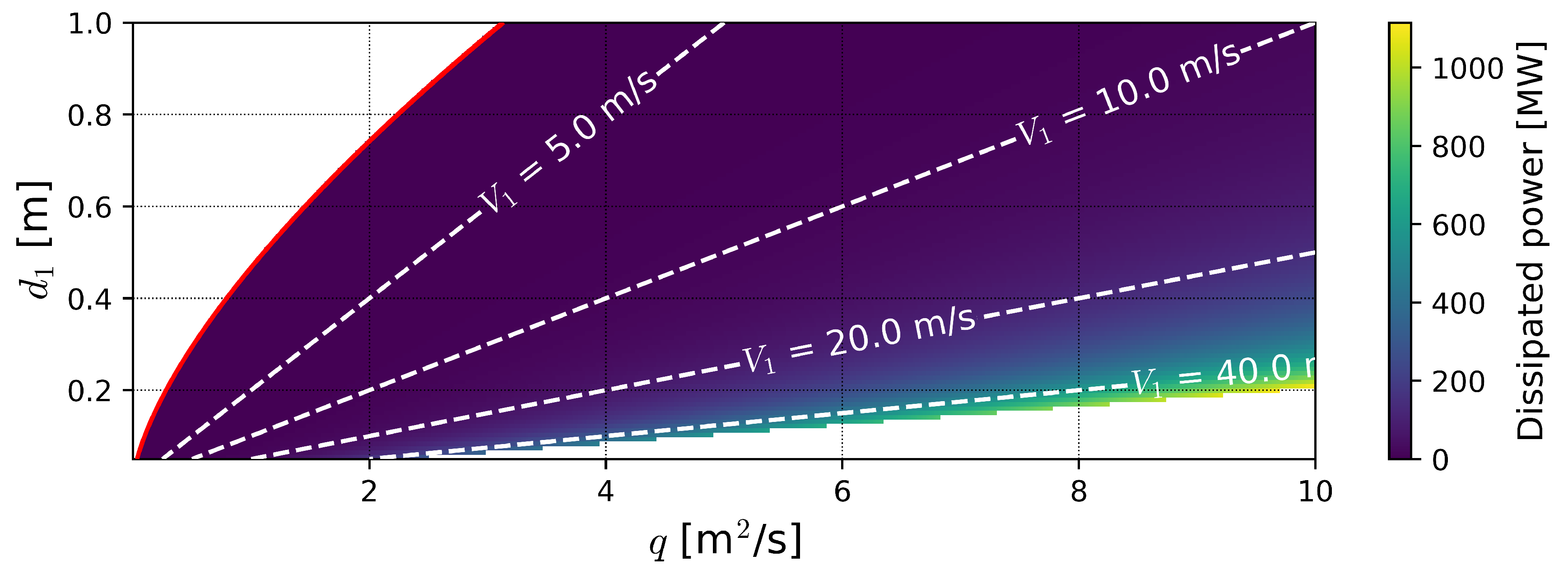
Once the flow depths upstream and downstream—and the flow rate—are known, the energy both upstream and downstream can be estimated and its difference is the energy dissipated. This also allows computation of the dissipated power ([42], p. 60). Figure 3 shows the dissipated power for a wide combination of flow discharges and inlet flow depths for a 100 m wide CHJ (frictionless). It must be noted that spillways wider than 100 m are not rare in prototype scale. It can be observed that dissipated power considerably increases for inlet velocities over 20 m/s. Power taking place in the energy dissipation of many dams is comparable to some of the world’s largest power stations [6]. Dissipated power values of a peak discharge may usually remain below a nuclear or a thermal power station power production (<1000 MW) but every linear meter remains easily over a wind turbine capacity (100 kW, or 10 MW for 100 m), as shown in Figure 3. It must be born in mind that all this dissipated power must be contained in a well delimited structure to ensure the stability of the downstream river and habitat and the safe operation of the dam.
2.2. Inflow Froude Number and Hydraulic Jump Typology
The Froude number is commonly used to classify the hydraulic jump typology. However, different authors define different classifications (see Table 1). Despite being slightly different, there is some overlap on the description of the hydraulic jumps’ typology. It is also commonly acknowledged that hydraulic jumps in the range 2 < < 4 should be avoided at design stage, as waves are generated and propagated downstream damaging the banks [22]. Thus, from an engineering point of view, hydraulic jumps with > 4–4.5 hold a greater interest. It must be noted that inflow conditions can also affect the hydraulic jumps’ typology [44], which could explain the small differences between authors (Table 1).
Undular jumps occur for upstream flow depths close to critical flow depth, but slightly below. This type of hydraulic jump exhibits several stationary waves, thus being morphologically different to higher Froude number hydraulic jumps. A lateral shock wave can also be observed starting with the first crest and considerably smaller rates of air entrainment occur. Undular jumps may occur in irrigation and water supply channels and in estuaries subject to tide changes [45]. For these types of hydraulic jumps, extensive experimental data can be found in Chanson [45].
2.3. Hydraulic Jump Flow Structure and Related Experimental Studies
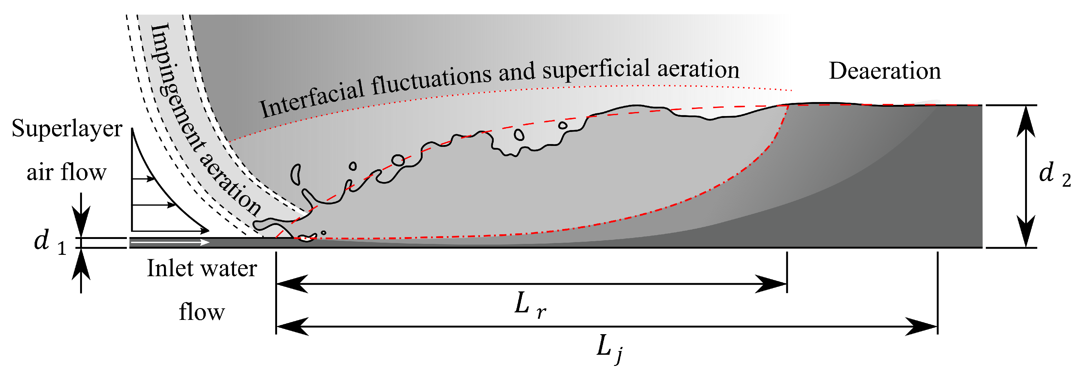
The hydraulic jump flow structure (Figure 4) mixes different types of simpler flows, leading to complex dynamics with large turbulence quantities and air entrainment. In addition to the sequent depth relation, other mean and turbulent flow features have been experimentally studied. A summary of previous studies including analytical, empirical relations or experimental data can be found in Table 2.
The reader is addressed to Wang [50] and Murzyn and Chanson [49] for a large experimental database—for several empirical relations, to Chanson and Carvalho [3] and Hager [2]. An up-to-date reference including a wide range of experimentally obtained flow variables (both mean and turbulent) can be found in the study of Wang and Chanson [51]. These studies might be very useful for the validation of numerical results. In addition, other experimental studies are relevant and are herein presented, highlighting the parameters that were mainly investigated:
- Wall jet velocity decay: the high-speed inlet flow impacts the slower moving water body and the shearing reduces the maximum velocity through the hydraulic jump length, likewise a turbulent wall jet decay. The shear layer also expands into the roller region. The analogy between hydraulic jumps and turbulent wall jets was first conducted by Rajaratnam [14]. This parameter is highly relevant as it holds the biggest part of the kinetic energy which, during the decay, is transformed into pressure and potential energy (depth). Experimental data can be found in Wang and Chanson [51], Chanson [56], Liu et al. [57], Chanson and Brattberg [16], Wu and Rajaratnam [58], Hager [2] and Ohtsu et al. [59].
- Roller length: marked in Figure 4 as , it is one of the most distinctive features of a hydraulic jump. Some of the inflow uplifts to the free surface, reaching a stagnation point and reversing, hence falling back again to the toe, where it impacts with the inflow jet. As the stagnation point moves continuously, its visual estimation is affected from a certain uncertainty in a physical model. Experimental data can be found in Murzyn et al. [60]. Wang and Chanson [52], Carollo et al. [36] and Hager [2] presented a nearly parabolic experimental relationship.
- Hydraulic jump length: marked in Figure 4 as . Different methods have been discussed concerning its identification as, for instance: a horizontal free surface can be observed, a hydrostatic pressure distribution is established or where the hydraulic jump is fully deaerated. However, it is also difficult to estimate as the free surface is wavy downstream and tends smoothly to horizontal, which implies a large degree of uncertainty. Pressure distribution is not commonly measured and deaeration may strongly depend on the modelling scale. Bayon et al. [61] argued that the turbulence produced in the toe of the hydraulic jump tended at the end of the hydraulic jump to the values commonly observed in open channel flows, but, for an experimental study, this is even more rare to measure. Given the difficulty of all these methods, visual determination is oftentimes the experimentalist preferred choice.
- Mean free surface profile: it necessarily matches the supercritical flow depth at the toe while it asymptotically tends to the downstream water depth at the end of the hydraulic jump. With an abrupt increase at the toe, it presents a concave curve during the hydraulic jump extension for Froude numbers over the undular jump limit (Table 1). In addition to the aforementioned studies, relations for this parameter were also suggested by Wang [50], Bakhmeteff and Matzke [12] and, analytically, by Valiani [55]. For undular jumps, experimental data can be found in Lennon and Hill [62] and analytical considerations were proposed by Bose et al. [63].
- Mean velocities: the high-speed jet entering the hydraulic jump splits, partly reversing and partly reducing its velocity, thus matching the downstream open channel flow velocity profile. This yields a complex velocity distribution zero-value-crossing at the roller region with an important negative velocity reaching a magnitude of up to 0.4 to 0.6 of the inlet velocity [3,56,64]. Recently, Wang and Chanson [51] suggested that this magnitude has an inverse relation with the Froude number. Empirical velocity distributions were proposed by Chanson and Carvalho [3] and Hager [2]. Literature is rich in experimental data too; see Wang and Chanson [51], Wang et al. [65], among others. Lin et al. [66] studied, separately, the velocity of the water and air phases by using Particle Image Velocimetry (PIV) and Bubble Image Velocimetry (BIV), alternatively. For undular jumps, experimental data can be found in Lennon and Hill [62].
- Aeration (impingement and interfacial): large quantities of air are entrained inside the hydraulic jump via the toe impingement. These large air volumes are subject to break-up and coalescence depending on the surrounding turbulence quantities. A second air entrainment mechanism is related to the interfacial fluctuations occurring in the upper region of the roller at higher Froude numbers. Large quantities of spray and splashing can be visually observed and have a clear footprint in the air concentration profiles. For both mechanisms, different air concentration profiles can be fitted, hence revealing different air entrainment mechanisms [67,68]. Far downstream, the flow deaerates as the velocity decreases and the transport capacity is reduced. The air concentration is, probably, one of the most case sensitive mean flow variables as it is a result of the combination of Froude, Reynolds and Weber—or equivalently, Morton—numbers [69]. Another reason for the case-sensitivity of the air entrained quantities should be related to the level of development of the inflow boundary layer, as reported by Takahashi and Ohtsu [70]. Takahashi and Ohtsu [70] noted that the advective diffusion region showed larger aeration, with greater development of the inlet boundary layer, while the (upper) breaking region was nearly insensitive to this variable. Ervine [71] also discussed on the relevance of the inlet flow free surface perturbations on the total air entrained. Moreover, the interaction between air bubbles diffusion and momentum transfer is not completely understood [68]. Air transport in the streamwise direction is mainly due to advection, whereas transport in the spanwise and normalwise direction is necessarily driven by turbulent diffusion. In the vertical direction, buoyant forces can also play an important role, especially at the end of the hydraulic jump where lower velocities occur. Experimental data on air concentrations and different semi-empirical relations can be found in Wang and Chanson [51], Takahashi and Ohtsu [70], Gualtieri and Chanson [68], Murzyn et al. [67], Chanson and Brattberg [16], among others.
- Inlet boundary layers (water and air): the supercritical flow impacting the hydraulic jump develops from farther upstream as long as its extension allows. Two boundary layers take place, the water boundary layer that can affect the hydraulic jump characteristics [44,70]—and thus it is common to distinguish between partially developed and fully developed inlet flows—and the interfacial air layer flow [72], which could affect the hydraulic jump air entrained quantities according to Ervine [71]. For the supercritical water boundary layer development, several methods exist, such as Castro-Orgaz and Hager [73] and Castro-Orgaz [74] based on spillway prototype scale velocity profiles. For the interfacial air flow, the only data-set was collected by Valero and Bung [72], which also discussed on the occurring free surface instabilities in supercritical flows that were suggested by Ervine [71] to affect the entrained quantities. A general framework for the computation of the free surface perturbations can be found in Valero and Bung [75]. Recently, Bertola et al. [76] showed that inlet disturbances considerably affect the air entrainment rates for planar plunging jets.
Some turbulent variables have also been previously experimentally studied:
- Velocity fluctuations: given the turbulent nature of hydraulic jumps, instantaneous velocities oscillate around the mean value. Velocity fluctuations were first reported by Rouse et al. [13] using an air flow channel. Long et al. [77] studied velocity fluctuations in submerged hydraulic jumps for Froude numbers up to 8.0, highlighting the three-dimensional nature of the hydraulic jump; and Liu et al. [57] presented turbulence measurements for low Froude numbers, including turbulence spectra. Turbulence intensity has also been approximated using the width of the cross-correlation function between the signals of the two tips of phase detection probes; see Chanson and Toombes [78] for further description and limitations and study of Murzyn and Chanson [49] for an application to hydraulic jumps. For undular jumps, experimental data were collected by Lennon and Hill [62]. Velocity fluctuations are of utmost interest to ensure the stability of downstream environment.
- Interfacial oscillations: the hydraulic jump free surface shows a wide range of turbulent motions. These oscillations play an important role in the study of the total air entrained in the hydraulic jump, as discussed above. Recently, some experimental studies have found that the maximum oscillation occurs close to the toe location and that the intensity of these oscillations increases with the Froude number. Experimental data can be found in Wang and Chanson [51], Chachereau and Chanson [79], Murzyn and Chanson [80].
- Toe oscillations: the roller flow backwards periodically as a consequence of all the hydrodynamic processes that occur inside the hydraulic jump. The Strouhal number (dimensionless frequency based on the toe frequency, inflow depth and mean velocity) is oftentimes used to describe this phenomenon. Toe oscillations have been reported by Zhang et al. [64], Chachereau and Chanson [79], Chanson and Gualtieri [69], Gualtieri and Chanson [68], Mossa and Tolve [81], and Long et al. [82].
- Large vortices advection: large vortices are created in the shear region between the inlet high-speed jet and the roller (vortex shedding). These are advected downstream with a velocity around 0.4 times the inlet velocity. It has not been noticed a clear effect of the Reynolds number. Experimental data can be found in Chanson [56] and Wang [50].
- Pressure fluctuations: the high-speed inlet jet has an impact against the slower water body abruptly slowing down while transforming some of the kinetic energy into pressure, which is later converted into potential energy (in the form of increasing depth). Considerable turbulent pressure fluctuations occur inside the hydraulic jump, thereby compromising the structural stability. Fiorotto and Rinaldo [83] discussed on the spatial structure and magnitude of these pressure oscillations at the channel bed level. Abdul Khader and Elango [84], additionally, also provided insight on the pressures spectra. Hydraulic jump related high pressure fluctuations also have a complex impact on the hyporheic flows occurring in river flows [4,5]. Special care must be taken to properly understand some recent experimental data reporting results on total pressure, which accounts both for the pressure and the velocity head and needs to be corrected with simultaneous velocity estimations and air concentrations to extract the real pressure head. Further description on this technique applied to hydraulic jumps can be found in Wang et al. [65,85] and Wang [50].
- Hydraulic jump vorticity: it is produced at the toe of the hydraulic jump. The inlet flow is abruptly subject to large shearing quantities after impinging the roller flow. The shearing reduces as the flow advances streamwise and the turbulence produced in the toe is slowly dissipated. Hornung et al. [86] analytically studied the mean vorticity downstream of a hydraulic jump and its relation with the Froude number.
- Inner turbulent structures: turbulent length and timescales have been measured using arrays of conductivity probes. Several synchronized sensors can be placed inside the flow and correlation of two signals allow a certain physical insight. Integration of the correlation functions (across time or spatial lag) leads to the estimation of the integral turbulent scales (temporary and spatial scales, respectively). These turbulent scales can be understood as an average measure of the turbulent structures taking place inside the hydraulic jump. A complete data bench of experimental data can be found in Wang and Murzyn [17].
- Bubble characteristics: bubble frequencies, chord lengths and times and bubble clustering are the result of an interaction among turbulent processes. Its determination may be one of the most challenging—if not the most—for a numerical model. These variables have been, however, reported in some experimental studies (e.g., [67,68,87,88]).
3. Adequacy of the Hydraulic Jump as a Benchmark for Numerical Modelling
As discussed by Blocken and Gualtieri [89], the interest of the hydraulic and environmental engineers about computational fluid dynamics (CFD) methods is shifted from the typical aerodynamics problems. Analysis is commonly focused on problems where turbulence is desired to mix mass or dissipate energy. Hence, the most common applications may require study of highly turbulent problems, such as hydraulic jumps which has been very present in the hydraulic engineering tradition.
The energy dissipation involved in these types of phenomenon is large, as discussed in Section 2.1, and, additionally, its modelling involves the proper solution of both supercritical and subcritical flows, with supercritical flows being prone to large free surface distortion [75]. Similarly, the hydraulic jump comprehends a shear region of large turbulence intensity with free surface interaction, leading to breakup and splashing. All in all, the CHJ represents a well-studied benchmark that serves as a limiting case in terms of free surface complexity and turbulence production. Other previous benchmarks have been conducted in the past (see [90]), but the types of flows contained within the hydraulic jump better represent those of greater interest for hydraulic and environmental engineers. These points justify the interest on CHJ as a reference for numerical modelling validation, and can be summarized as:
- Deep understanding of the phenomenon, as presented in Section 2.3.
- Large hydraulic tradition, which makes most of the community familiar with this type of flow.
- It represents an extreme case for turbulence, aeration and flow recirculation, which ensures that numerical models representing properly a CHJ are likely to be useful for other environmental applications.
4. Discussion on Experimental Uncertainties
While a scaled physical model is better suited to represent the real behaviour of a fluid system, there are some limitations due to the scale effects and the instrumentation inaccuracies. Both can represent a strong limitation in the case of air–water flow problems and thus, when the purpose of a numerical study is the verification and validation of the model, the exact same physical model is preferred to be reproduced and contemplating the employed instrumentations’ uncertainties may help identifying a reasonable accuracy goal for the validation of the numerical studies. Instrumentation limitations are considerably stronger in air–water flows when compared to the counterpart single-phase flows. On the limitations that scale effects represent, the reader is addressed to Chanson and Gualtieri [69], Chanson [91], Felder and Chanson [92] and Felder and Chanson [93]. On the limitations of instrumentation for air–water flows, a brief summary with relevant references is presented in Table 3.
Point gauges have been traditionally used to estimate the flow depths. Nonetheless, the free surface fluctuations occur not only within the hydraulic jump but also at the upstream and downstream ends. The accuracy of classic point gauges is often referred to be in the order of 0.1 mm; however, this can only hold for static water levels. Oscillations are common within the hydraulic jump, but they can also be observed downstream (due to the waves propagated) and in the upstream supercritical flow depth (due to perturbations).
Under such conditions, the flow depth estimation holds a considerable observation error. Another type of instrumentation, which is used more everyday for flow depth estimations, is the ultrasonic sensors (USS), also called acoustic displacement meters (ADM) by some authors. These sensors create an echo that propagates in the air and measure the time it takes to be received back. It allows a dynamic estimation of the free surface, timely limited by the response time of the sensor and the time it takes to propagate the ultrasonic echo (which is represented by a cutoff frequency). The recent study of Zhang et al. [94] analysed the accuracy of such devices for steady, two-dimensional and three-dimensional waves, concluding that the accuracy is reasonably good despite the minimum wavelength that can be detected is a function of the footprint of the sensors. This may imply that some droplets can be ignored; however, Zhang et al. [94] also noted that upper surfaces are given preference and larger inaccuracies can be expected when flow is aerated. A critical slope exists, hence limiting non-horizontal free surfaces determination and yielding outliers in the recording. For the free surface determination, Light Detection and Ranging (LiDAR) technique has shown to be promising, allowing the simultaneous temporal and spatial series estimations [95], despite appropriate filtering might be critical.
Acoustic Doppler Velocimeters (ADV) have also been used to measure velocities in hydraulic jumps, but its accuracy is highly handicapped by the presence of bubbles and its use is not recommended even for very low concentrations. Discussion on ADV’s accuracy can be found in Liu et al. [57]. Additionally, postprocessing techniques are necessary to ensure accurate turbulence predictions (e.g., [106]). Some recently developed ADV models also incorporate a ”profiling” option, which allows simultaneously obtaining velocity estimations at a distance range. However, different issues have already been noticed, such as non-overlapping profiles or non-null transversal velocities (see [107]).
When air concentrations amount to over a few percent, the preferred instrumentation should be phase detection probes [96,97]. Special care must be taken in regions with near null velocities and important cross velocities, which lead to oblique impact of bubbles with the probes’ tips or bubbles undetected by at least one tip (impacting the cross-correlation performance). The first direct turbulence estimation with phase detection probes in highly aerated flows has been recently presented by Kramer et al. [98] through an adaptive cross-correlation approach coupled with robust filtering techniques. However, these findings are yet limited to a stepped spillway model.
Optical methods have also been used in aerated flows, the Bubble Image Velocimetry being the Particle Image Velocimetry version for aerated flows; however, the accuracy reached is not comparable. Computer Vision methods (such as Optical Flow) are arising as a robust alternative for air–water flows [102,103,104,105,108].
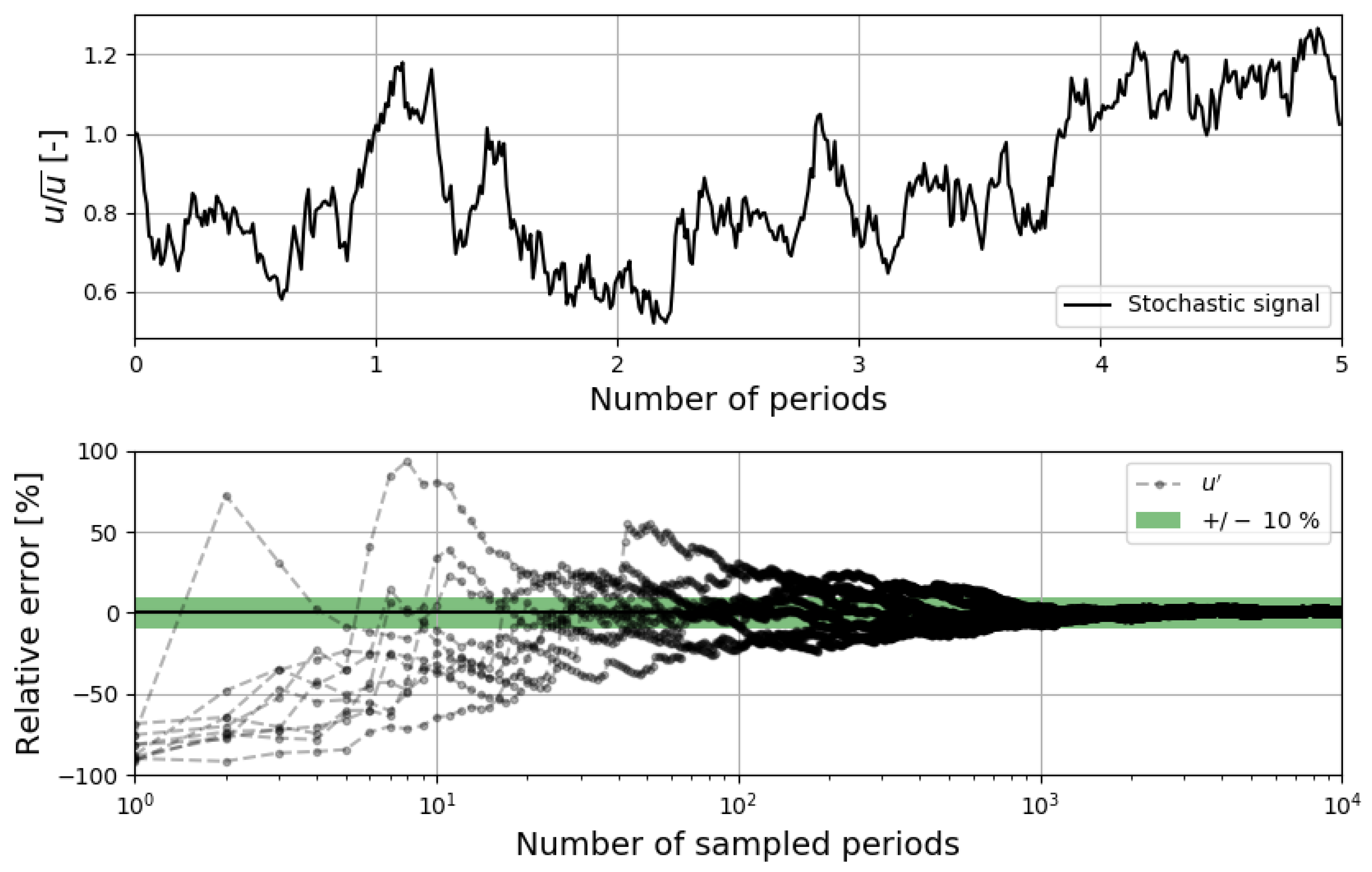
In addition to the instrumentation limitations and the outliers present in the data, a perfectly sampled data series would still present uncertainties related to the limitations on the sampling time or the sampling rate. Figure 5 shows an estimation of the error due to limited sampled time for a stochastic velocity signal (instantaneous velocity u, mean velocity = 1 m/s, velocity mean fluctuation = 0.3 m/s, characteristic timescale of 1 s, generated using the Langevin equation likewise Bung and Valero [108] and Kramer et al. [98]). The error in Figure 5 is computed relative to the estimation using the entire signal, which contains a total of 100,000 periods with a time resolution of 100 data points per period. The flow parameters are representative of a typical hydraulic jump at the laboratory scale. It can be observed that at least 1000 periods should be sampled to obtain an uncertainty below 10% for perfectly sampled data. Similar conclusions could be drawn from the analysis of the limited sample rate and its impact on the estimation of the turbulent timescales.
5. Conclusions
Hydraulic jumps represent one of the most turbulent and challenging canonical types of flow, characterized by strong multi-phase interactions. Its flow structure mixes different types of interacting conventional flows, e.g., boundary layers, shear regions and multiple phenomenon associated with the bubbles’ dynamics. Opportunely, experimental studies have covered various mean and turbulent flow variables, which, as herein proposed, may serve as a suitable workbench of CFD codes.
Numerous mean flow variables have been extensively studied in past literature, namely: sequent depths’ relationship, maximum velocity decay, roller length, jump length, mean free surface profile, mean velocity profiles and air concentrations (despite some are linked to flow turbulence). These variables should constitute the minimum dataset for numerical models’ validation. Studies of Hager [2], Murzyn and Chanson [49] and Wang [50] stand out due to the large number of variables covered and the extensive experimental datasets presented. These three experimental data collections, together with additional complementary studies, are pinpointed in Table 2. Turbulent variables have also been the object of several experimental studies. These may serve to better validate numerical models, despite the fact that their study has not been that systematic (Section 2.3).
It is also important to bear in mind that hydraulic jumps are multiphase flow problems, with high levels of aeration which represent a challenge for traditional single-phase instrumentation. Most of the equipment used in classic water-flow problems fail to provide accurate estimations for simple flow variables. The presence of bubbles make difficult the application of well-established techniques such as PIV or ADV. Section 4 depicts the main difficulties of a wide range of instrumentation and directs the reader to several key studies (Table 3). Other uncertainties may hold as, for instance, scale effects or laboratory inflow/outflow effects. Modelling the flow problem with the same geometry of the experimental study, just for validation purposes, may overcome these issues. Limited sampling time can also imply a certain level of uncertainty on the reported flow variables (Figure 5).
Part 2 [26] of this study presents the main achievements in the three-dimensional numerical modelling of hydraulic jumps.
Author Contributions
Conceptualization, D.V. and C.G.; Writing—Original Draft Preparation, D.V. and N.V.; Writing—Review and Editing, D.V. and C.G.
Funding
This research was funded by [Regione Campania] grant number [E66DO80007002].
Acknowledgments
Nicolò Viti acknowledges the support from the Project ”Sistemi avanzati di dissipazione a risalto nelle opere idrauliche: aspetti teorici e progettuali” funded from the Regione Campania under the ”L.R. n. 5 del 28/03/1992”.
Conflicts of Interest
The authors declare no conflict of interest.
References
- Rajaratnam, N. Hydraulic Jumps. Adv. Hydrosci. 1967, 4, 197–280. [Google Scholar] [CrossRef]
- Hager, W.H. Energy Dissipators and Hydraulic Jump; Water Science and Technology Library; Springer Science & Business Media: Dordrecht, The Netherlands, 1992; Volume 8, ISBN 978-90-481-4106-7. [Google Scholar]
- Chanson, H.; Carvalho, R. Hydraulic jumps and stilling basins. In Energy Dissipation in Hydraulic Structures; Chanson, H., Ed.; CRC Press: Leiden, The Netherlands, 2015; pp. 65–104. ISBN 978-1-138-02755-8. [Google Scholar] [Green Version]
- Endreny, T.; Lautz, L.; Siegel, D.I. Hyporheic flow path response to hydraulic jumps at river steps: Flume and hydrodynamic models. Water Resour. Res. 2011, 47, 2517. [Google Scholar] [CrossRef]
- Endreny, T.; Lautz, L.; Siegel, D.I. Hyporheic flow path response to hydraulic jumps at river steps: Hydrostatic model simulations. Water Resour. Res. 2011, 47, 2518. [Google Scholar] [CrossRef]
- Chanson, H. Energy Dissipation in Hydraulic Structures; CRC Press: Leiden, The Netherlands, 2015; ISBN 978-1-138-02755-8. [Google Scholar]
- Bidone, G. Expériences sur la propagation des remous. Memorie della Reale Accademia de/le Scienze di Torino 1820, 30, 195–292. [Google Scholar]
- Mossa, M.; Petrillo, A. A brief history of the jump of Bidone. In XXX IAHR Congress: August 2003, Thessaloniki, Greece; Ganoulis, J., Prinos, P., Armamimi, A., Latinopoulos, P., Eds.; International Association for Hydraulic Engineering and Research (IAHR): Thessaloniki, Greece, 2003. [Google Scholar]
- Bélanger, J.B. Essai sur la Solution NuméRique de Quelques ProblèMes Relatifs au Mouvement Permanent des Eaux Courantes; Carilian-Goeury: Paris, France, 1828. [Google Scholar]
- Chanson, H. Development of the Bélanger equation and backwater equation by Jean-Baptiste Bélanger (1828). J. Hydraul. Eng. 2009, 135, 159–163. [Google Scholar] [CrossRef]
- Bidone, G. Notes sur l’hydraulique; École Royale des Ponts et Chaussées: Champs-sur-Marne, France, 1841. [Google Scholar]
- Bakhmeteff, B.A.; Matzke, A.E. The hydraulic jump in terms of dynamic similarity. ASCE Trans. 1936, 101, 630–647. [Google Scholar]
- Rouse, H.; Siao, T.T.; Nagaratnam, S. Turbulence characteristics of the hydraulic jump. J. Hydraul. Div. ASCE 1958, 84, 1–30. [Google Scholar]
- Rajaratnam, N. The hydraulic jump as a wall jet. J. Hydraul. Div. ASCE 1965, 91, 107–132. [Google Scholar]
- Resch, F.J.; Leutheusser, H.J. Reynolds stress measurements in hydraulic jumps. J. Hydraul. Res. 1972, 10, 409–429. [Google Scholar] [CrossRef]
- Chanson, H.; Brattberg, T. Experimental study of the air–water shear flow in a hydraulic jump. Int. J. Multiph. Flow 2000, 26, 583–607. [Google Scholar] [CrossRef] [Green Version]
- Wang, H.; Murzyn, F. Experimental assessment of characteristic turbulent scales in two-phase flow of hydraulic jump: From bottom to free surface. Environ. Fluid Mech. 2017, 17, 7–25. [Google Scholar] [CrossRef]
- Warnock, J.E. Spillways and Energy Dissipators. In Proceedings of the Hydraulic Conference, Iowa City, IA, USA, 12–15 June 1939. [Google Scholar]
- Ead, S.A.; Rajaratnam, N. Hydraulic jumps on corrugated beds. J. Hydraul. Eng. 2002, 128, 656–663. [Google Scholar] [CrossRef]
- Pagliara, S.; Lotti, I.; Palermo, M. Hydraulic jump on rough bed of stream rehabilitation structures. J. Hydro-Environ. Res. 2008, 2, 29–38. [Google Scholar] [CrossRef]
- Felder, S.; Chanson, H. Air-Water Flow Patterns of Hydraulic Jumps on Uniform Beds Macroroughness. J. Hydraul. Eng. 2018, 144, 04017068. [Google Scholar] [CrossRef]
- Peterka, A.J. Hydraulic Design of Stilling Basins and Energy Dissipators; Department of the Interior, Bureau of Reclamation: Washington, DC, USA, 1978.
- Blaisdell, F.W. The SAF Stilling Basin: A Structure to Dissipate the Destructive Energy in High-Velocity Flow from Spillways; Agriculture Handbook No. 156; United States Department of Agriculture: Washington, DC, USA, 1959.
- Chanson, H.; Lubin, P. Discussion of Verification and validation of a computational fluid dynamics (CFD) model for air entrainment at spillway aerators. Can. J. Civ. Eng. 2010, 37, 135–138. [Google Scholar] [CrossRef]
- Chanson, H. Hydraulics of aerated flows: Qui pro quo? J. Hydraul. Res. 2013, 51, 223–243. [Google Scholar] [CrossRef]
- Viti, N.; Valero, D.; Gualtieri, C. Numerical Simulation of Hydraulic Jumps. Part 2: Recent Results and Future Outlook. Water 2019, 11, 28. [Google Scholar] [CrossRef]
- Kabiri-Samani, A.; Rabiei, M.H.; Safavi, H.; Borghei, S.M. Experimental-analytical investigation of super-to subcritical flow transition without a hydraulic jump. J. Hydraul. Res. 2014, 52, 129–136. [Google Scholar] [CrossRef]
- Kabiri-Samani, A.; Naderi, S. Turbulent structure in the transition from super-to subcritical flow without a hydraulic jump. J. Hydraul. Res. 2017, 55, 50–62. [Google Scholar] [CrossRef]
- Koch, C.; Chanson, H. Turbulence measurements in positive surges and bores. J. Hydraul. Res. 2009, 47, 29–40. [Google Scholar] [CrossRef] [Green Version]
- Gualtieri, C.; Chanson, H. Experimental study of a positive surge. Part 2: Comparison with literature theories and unsteady flow field analysis. Environ. Fluid Mech. 2011, 11, 641–651. [Google Scholar] [CrossRef]
- Gualtieri, C.; Chanson, H. Experimental study of a positive surge. Part 1: Basic flow patterns and wave attenuation. Environ. Fluid Mech. 2012, 12, 145–159. [Google Scholar] [CrossRef]
- Leng, X.; Chanson, H. Breaking bore: Physical observations of roller characteristics. Mech. Res. Commun. 2015, 65, 24–29. [Google Scholar] [CrossRef] [Green Version]
- Leng, X.; Chanson, H. Unsteady velocity profiling in bores and positive surges. Flow Meas. Instrum. 2017, 54, 136–145. [Google Scholar] [CrossRef] [Green Version]
- Chanson, H. Momentum considerations in hydraulic jumps and bores. J. Irrig. Drain. Eng. 2012, 138, 382–385. [Google Scholar] [CrossRef]
- Hager, W.H.; Bremen, R. Classical hydraulic jump: Sequent depths. J. Hydraul. Res. 1989, 27, 565–585. [Google Scholar] [CrossRef]
- Carollo, F.G.; Ferro, V.; Pampalone, V. New solution of classical hydraulic jump. J. Hydraul. Eng. 2009, 135, 565–585. [Google Scholar] [CrossRef]
- Pagliara, S.; Palermo, M. Hydraulic jumps on rough and smooth beds: Aggregate approach for horizontal and adverse-sloped beds. J. Hydraul. Res. 2015, 53, 243–252. [Google Scholar] [CrossRef]
- Palermo, M.; Pagliara, S. Semi-theoretical approach for energy dissipation estimation at hydraulic jumps in rough sloped channels. J. Hydraul. Res. 2018, 56, 786–795. [Google Scholar] [CrossRef]
- Felder, S.; Chanson, H. An Experimental Study of Air-Water Flows in Hydraulic Jumps with Channel Bed Roughness; UNSW Report No. WRL 259; Water Research Laboratory: Allambie Heights, Australia, 2016. [Google Scholar]
- Frizell, K.W.; Svoboda, C.D. Performance of Type III Stilling Basins-Stepped Spillway Studies: Do Stepped Spillways Affect Traditional Design Parameters? US Department of the Interior, Bureau of Reclamation: Washington, DC, USA, 2012.
- Valero, D.; Bung, D.B.; Crookston, B.M. Energy dissipation of a Type III basin under design and adverse conditions for stepped and smooth spillways. J. Hydraul. Eng. 2018, 144, 04018036. [Google Scholar] [CrossRef]
- Chanson, H. The Hydraulics of Open Channel Flow: An Introduction, 2nd ed.; Butterworth-Heinemann: Oxford, UK, 2004; ISBN 978-0750659789. [Google Scholar]
- Valero, D.; Fullana, O.; Gacía-Bartual, R.; Andrés-Domenech, I.; Valles, F. Analytical formulation for the aerated hydraulic jump and physical modelling comparison. In Proceedings of the 3rd IAHR Europe Congress, Porto, Portugal, 14–16 April 2014. [Google Scholar]
- Chanson, H. Air-Water Gas Transfer at Hydraulic Jump with Partially Developed Inflow. Water Res. 1995, 29, 2247–2254. [Google Scholar] [CrossRef]
- Chanson, H. Flow Characteristics of Undular Hydraulic Jumps. Comparison With Near-Critical Flows; CH45/95; Department of Civil Engineering, The University of Queensland: Brisbane, QLD, Australia, 1995. [Google Scholar]
- Bradley, J.N.; Peterka, A.J. Hydraulic Design of Stilling Basins. J. Hydraul. Div. ASCE 1957, 83, 1401–1406. [Google Scholar]
- Chow, V.T. Hydraulics of Open Channel Flow; American Society of Civil Engineers (ASCE) Press: Reston, VA, USA, 1998. [Google Scholar]
- Chow, V.T. Open Channel Hydraulics; McGraw-Hill: New York, NY, USA, 1973. [Google Scholar]
- Murzyn, F.; Chanson, H. Free Surface, Bubbly Flow and Turbulence Measurements in Hydraulic Jumps; CH63/07; Department of Civil Engineering, The University of Queensland: Brisbane, QLD, Australia, 2007. [Google Scholar]
- Wang, H. Turbulence and Air Entrainment in Hydraulic Jumps. Ph.D. Thesis, Department of Civil Engineering, The University of Queensland, Brisbane, QLD, Australia, 2014. [Google Scholar]
- Wang, H.; Chanson, H. Energy Self-similarity and scale effects in physical modelling of hydraulic jump roller dynamics, air entrainment and turbulent scales. Environ. Fluid Mech. 2016, 16, 1087–1110. [Google Scholar] [CrossRef]
- Wang, H.; Chanson, H. Experimental study of turbulent fluctuations in hydraulic jumps. J. Hydraul. Eng. 2015, 141, 04015010. [Google Scholar] [CrossRef]
- Carollo, F.G.; Ferro, V.; Pampalone, V. New expression of the hydraulic jump roller length. J. Hydraul. Eng. 2012, 138, 995–999. [Google Scholar] [CrossRef]
- Schulz, H.E.; Simões, A.L.A.; Nóbrega, J.D. Roller lengths, sequent depths, surface profiles for pre-design of dissipation basins. In Proceedings of the 2nd International Workshop on Hydraulic Structures: Data Validation, Coimbra, Portugal, 7–9 May 2015. [Google Scholar]
- Valiani, A. Linear and angular momentum conservation in hydraulic jump. J. Hydraul. Res. 1997, 35, 323–354. [Google Scholar] [CrossRef]
- Chanson, H. Convective transport of air bubbles in strong hydraulic jumps. Int. J. Multiph. Flow 2010, 36, 798–814. [Google Scholar] [CrossRef] [Green Version]
- Liu, M.; Rajaratnam, N.; Zhu, D.Z. Turbulence structure of hydraulic jumps of low Froude numbers. J. Hydraul. Eng. 2004, 130, 511–520. [Google Scholar] [CrossRef]
- Wu, S.; Rajaratnam, N. Free jumps, submerged jumps and wall jets. J. Hydraul. Res. 1995, 33, 197–212. [Google Scholar] [CrossRef]
- Ohtsu, I.; Koike, M.; Yasuda, Y.; Awazu, S.; Yamanaka, T. Free and Submerged Hydraulic Jumps in Rectangular Channels; Report of Research Institute of Science and Technology, No. 35; Nihon University: Tokyo, Japan, 1990. [Google Scholar]
- Murzyn, F.; Mouaze, D.; Chaplin, J.R. Air-water interface dynamic and free surface features in hydraulic jumps. J. Hydraul. Res. 2007, 45, 679–685. [Google Scholar] [CrossRef]
- Bayon, A.; Valero, D.; García-Bartual, R.; Vallés-Morán, F.J.; López-Jiménez, P.A. Performance assessment of OpenFOAM and FLOW-3D in the numerical modeling of a low Reynolds number hydraulic jump. Environ. Soft. 2016, 80, 322–335. [Google Scholar] [CrossRef]
- Lennon, J.M.; Hill, D. Particle image velocity measurements of undular and hydraulic jumps. J. Hydraul. Eng. 2006, 132, 1283-0-1294. [Google Scholar] [CrossRef]
- Bose, S.K.; Castro-Orgaz, O.; Dey, S. Free surface profiles of undular hydraulic jumps. J. Hydraul. Eng. 2011, 138, 362–366. [Google Scholar] [CrossRef]
- Zhang, G.; Wang, H.; Chanson, H. Turbulence and aeration in hydraulic jumps: Free-surface fluctuation and integral turbulent scale measurements. Environ. Fluid Mech. 2013, 13, 189–204. [Google Scholar] [CrossRef]
- Wang, H.; Murzyn, F.; Chanson, H. Total pressure fluctuations and two-phase flow turbulence in hydraulic jumps. Exp. Fluids 2014, 55, 1847. [Google Scholar] [CrossRef] [Green Version]
- Lin, C.; Hsieh, S.C.; Lin, I.J.; Chang, K.A.; Raikar, R.V. Flow property and self-similarity in steady hydraulic jumps. Exp. Fluids 2012, 53, 1591–1616. [Google Scholar] [CrossRef]
- Murzyn, F.; Mouaze, D.; Chaplin, J.R. Optical fibre probe measurements of bubbly flow in hydraulic jumps. Int. J. Multiph. Flow 2005, 31, 141–154. [Google Scholar] [CrossRef]
- Gualtieri, C.; Chanson, H. Experimental analysis of Froude number effect on air entrainment in the hydraulic jump. Environ. Fluid Mech. 2007, 7, 217–238. [Google Scholar] [CrossRef] [Green Version]
- Chanson, H.; Gualtieri, C. Similitude and scale effects of air entrainment in hydraulic jumps. J. Hydraul. Res. 2013, 46, 35–44. [Google Scholar] [CrossRef]
- Takahashi, M.; Ohtsu, I. Effects of inflows on air entrainment in hydraulic jumps below a gate. J. Hydraul. Res. 2017, 55, 259–268. [Google Scholar] [CrossRef]
- Ervine, D.A. Air entrainment in hydraulic structures: A review. Proc. Inst. Civ. Engrs Water Marit. Energy 1998, 130, 142–153. [Google Scholar] [CrossRef]
- Valero, D.; Bung, D.B. Development of the interfacial air layer in the non-aerated region of high-velocity spillway flows. Instabilities growth, entrapped air and influence on the self-aeration onset. Int. J. Multiph. Flow 2016, 84, 66–74. [Google Scholar] [CrossRef]
- Castro-Orgaz, O.; Hager, W.H. Drawdown curve and turbulent boundary layer development for chute flow. J. Hydraul. Res. 2010, 48, 591–602. [Google Scholar] [CrossRef] [Green Version]
- Castro-Orgaz, O. Velocity profile and flow resistance models for developing chute flow. J. Hydraul. Eng. 2009, 136, 447–452. [Google Scholar] [CrossRef]
- Valero, D.; Bung, D.B. Reformulating self-aeration in hydraulic structures: Turbulent growth of free surface perturbations leading to air entrainment. Int. J. Multiph. Flow 2018, 100, 127–142. [Google Scholar] [CrossRef]
- Bertola, N.; Wang, H.; Chanson, H. A physical study of air–water flow in planar plunging water jet with large inflow distance. Int. J. Multiph. Flow 2018, 100, 155–171. [Google Scholar] [CrossRef] [Green Version]
- Long, D.; Steffler, P.M.; Rajaratnam, N. LDA study of flow structure in submerged hydraulic jump. J. Hydraul. Res. 1990, 28, 437–460. [Google Scholar] [CrossRef]
- Chanson, H.; Toombes, L. Air-water flows down stepped chutes: turbulence and flow structure observations. Int. J. Multiph. Flow 2018, 28, 1737–1761. [Google Scholar] [CrossRef]
- Chachereau, Y.; Chanson, H. Free-surface fluctuations and turbulence in hydraulic jumps. Exp. Therm. Fluid Sci. 2018, 35, 896–909. [Google Scholar] [CrossRef]
- Murzyn, F.; Chanson, H. Free-surface fluctuations in hydraulic jumps: Experimental observations. Exp. Therm. Fluid Sci. 2018, 33, 1055–1064. [Google Scholar] [CrossRef]
- Mossa, M.; Tolve, U. Flow visualization in bubbly two-phase hydraulic jump. J. Fluids Eng. 1998, 120, 160–165. [Google Scholar] [CrossRef]
- Long, D.; Rajaratnam, N.; Steffler, P.M.; Smy, P.R. Structure of flow in hydraulic jumps. J. Hydraul. Res. 1991, 29, 207–218. [Google Scholar] [CrossRef]
- Fiorotto, V.; Rinaldo, A. Turbulent pressure fluctuations under hydraulic jumps. J. Hydraul. Res. 1992, 30, 499–520. [Google Scholar] [CrossRef]
- Abdul Khader, M.H.; Elango, K. Turbulent pressure field beneath a hydraulic jump. J. Hydraul. Res. 1992, 12, 469–489. [Google Scholar] [CrossRef]
- Wang, H.; Murzyn, F.; Chanson, H. Interaction between free-surface, two-phase flow and total pressure in hydraulic jump. Exp. Therm. Fluid Sci. 2015, 64, 30–41. [Google Scholar] [CrossRef] [Green Version]
- Hornung, H.G.; Willert, C.; Turner, S. The flow field downstream of a hydraulic jump. J. Fluid Mech. 1995, 287, 299–316. [Google Scholar] [CrossRef] [Green Version]
- Gualtieri, C.; Chanson, H. Effect of Froude number on bubble clustering in a hydraulic jump. J. Hydraul. Res. 2010, 48, 504–508. [Google Scholar] [CrossRef] [Green Version]
- Gualtieri, C.; Chanson, H. Interparticle arrival time analysis of bubble distributions in a dropshaft and hydraulic jump. J. Hydraul. Res. 2013, 51, 253–264. [Google Scholar] [CrossRef]
- Blocken, B.; Gualtieri, C. Ten iterative steps for model development and evaluation applied to Computational Fluid Dynamics for Environmental Fluid Mechanics. Environ. Soft. 2012, 33, 1–22. [Google Scholar] [CrossRef]
- Bradshaw, P.; Launder, B.E.; Lumley, J.L. Collaborative testing of turbulence models. J. Fluids Eng. 1996, 118, 243–247. [Google Scholar] [CrossRef]
- Chanson, H. Turbulent air–water flows in hydraulic structures: dynamic similarity and scale effects. Environ. Fluid Mech. 2009, 9, 125–142. [Google Scholar] [CrossRef]
- Felder, S.; Chanson, H. Turbulence, dynamic similarity and scale effects in high-velocity free-surface flows above a stepped chute. Exp. Fluids 2009, 47, 1–18. [Google Scholar] [CrossRef] [Green Version]
- Felder, S.; Chanson, H. Scale effects in microscopic air–water flow properties in high-velocity free-surface flows. Exp. Therm. Fluid Sci. 2017, 83, 19–36. [Google Scholar] [CrossRef]
- Zhang, G.; Valero, D.; Bung, D.B.; Chanson, H. On the estimation of free-surface turbulence using ultrasonic sensors. Flow Meas. Inst. 2018, 60, 171–184. [Google Scholar] [CrossRef] [Green Version]
- Montano, L.; Li, R.; Felder, S. Continuous measurements of time-varying free-surface profiles in aerated hydraulic jumps with a LIDAR. Exp. Therm. Fluid Sci. 2018, 93, 379–397. [Google Scholar] [CrossRef]
- Chanson, H. Phase-detection measurements in free-surface turbulent shear flows. J. Geophys. Eng. 2016, 13, S74. [Google Scholar] [CrossRef]
- Felder, S.; Pfister, M. Comparative analyses of phase-detective intrusive probes in high-velocity air–water flows. Int. J. Multiph. Flow 2017, 90, 88–101. [Google Scholar] [CrossRef]
- Kramer, M.; Valero, D.; Chanson, H.; Bung, D.B. Towards reliable turbulence estimations with phase‑detection probes: An adaptive window cross‑correlation technique. Exp. Fluids 2018. [Google Scholar] [CrossRef]
- Bung, D.B. Non-intrusive measuring of air–water flow properties in self-aerated stepped spillway flow. In Proceedings of the 34th IAHR World Congress, Brisbane, Australia, 26 June–1 July 2011. [Google Scholar]
- Leandro, J.; Bung, D.B.; Carvalho, R. Measuring void fraction and velocity fields of a stepped spillway for skimming flow using non-intrusive methods. Exp. Fluids 2014, 55, 1732. [Google Scholar] [CrossRef]
- Bung, D.B.; Valero, D. Image processing for bubble image velocimetry in self-aerated flows. In Proceedings of the 36th IAHR World Congress, The Hague, The Netherlands, 28 June–3 July 2015. [Google Scholar]
- Bung, D.B.; Valero, D. Optical flow estimation in aerated flows. J. Hydraul. Res. 2016, 54, 575–580. [Google Scholar] [CrossRef]
- Bung, D.B.; Valero, D. Application of the optical flow method to velocity determination in hydraulic structure models. In Proceedings of the 6th International Symposium on Hydraulic Structures, Portland, OR, USA, 27–30 June 2016. [Google Scholar]
- Bung, D.B.; Valero, D. Image processing techniques for velocity estimation in highly aerated flows: Bubble Image Velocimetry vs. Optical Flow. In Proceedings of the 4th IAHR Europe Congress, Liège, Belgium, 27–29 July 2016. [Google Scholar]
- Zhang, G.; Chanson, H. Application of local optical flow methods to high-velocity free-surface flows: Validation and application to stepped chutes. Exp. Therm. Fluid Sci. 2018, 90, 186–199. [Google Scholar] [CrossRef] [Green Version]
- Goring, D.G.; Nikora, V.I. Despiking acoustic Doppler velocimeter data. J. Hydraul. Eng. 2002, 128, 117–126. [Google Scholar] [CrossRef]
- Thomas, R.E.; Schindfessel, L.; McLelland, S.J.; Creëlle, S.; De Mulder, T. Bias in mean velocities and noise in variances and covariances measured using a multistatic acoustic profiler: The Nortek Vectrino Profiler. Meas. Sci. Technol. 2017, 28, 075302. [Google Scholar] [CrossRef]
- Bung, D.B.; Valero, D. FlowCV—An open source toolbox for computer vision applications in turbulent flows. In Proceedings of the 37th IAHR World Congress, Kuala Lumpur, Malaysia, 13–18 August 2017. [Google Scholar]
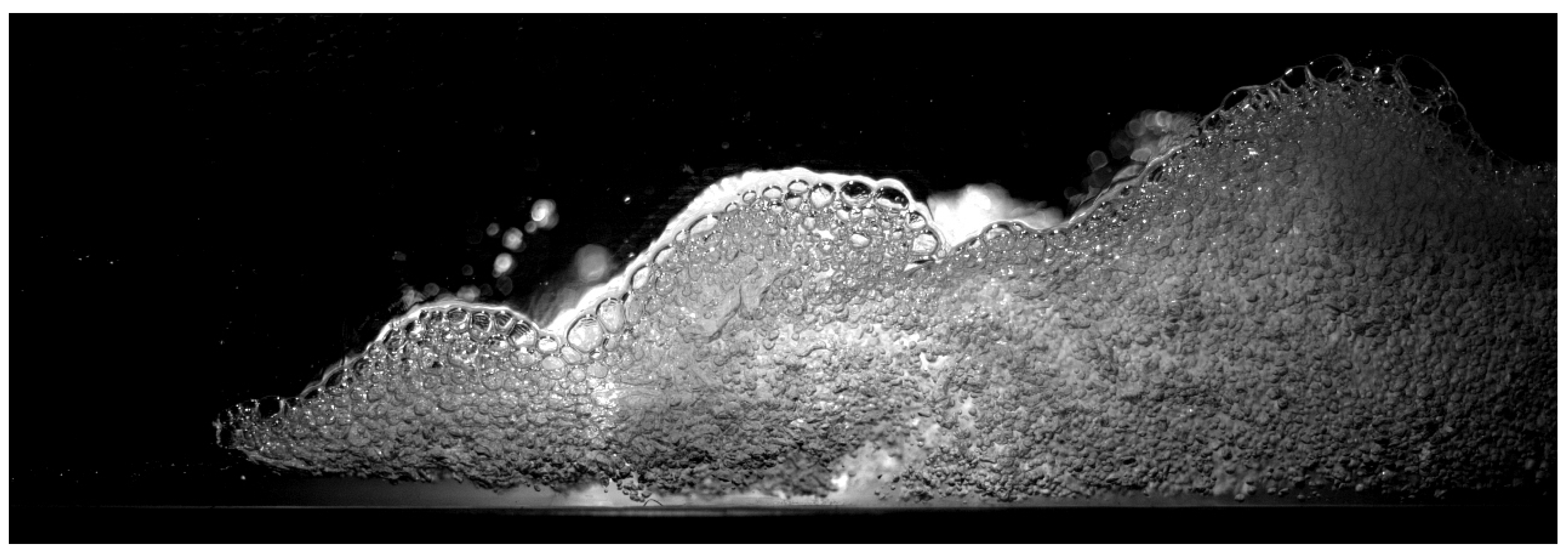
Figure 1.
Hydraulic jump at the Hydraulics Laboratory of The University of Queensland (inlet Froude number 7.5, flow from left to right). Courtesy of Dr. Wang.
Figure 1.
Hydraulic jump at the Hydraulics Laboratory of The University of Queensland (inlet Froude number 7.5, flow from left to right). Courtesy of Dr. Wang.

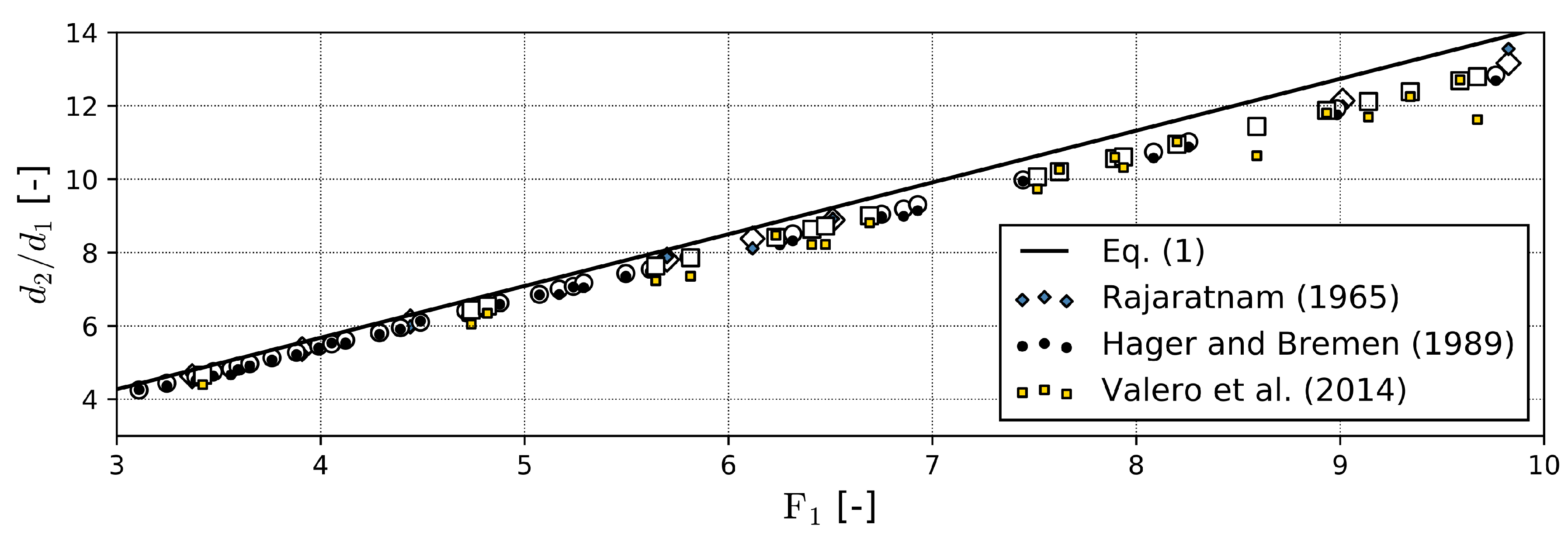
Figure 2.
Experimental data (small solid markers) against theoretical predictions of Bélanger equation (Equation (1)) and Hager and Bremen theoretical formulation (big empty markers). Note that Hager and Bremen [35] formulation is Reynolds number and width/depth ratio dependent, and thus a solid line cannot be traced. Median absolute relative difference between Hager and Bremen [35] formulation and experimental data of: Rajaratnam [14] 2.20%; Hager and Bremen [35] 1.36%; and Valero et al. [43] 3.27%.

Figure 3.
Dissipated energy in a 100 m wide Classic hydraulic jump (CHJ) depending on the inflow conditions: depth and specific flow rate q. Values for = 1 have been marked with a red solid line. Discharges with > 50 m/s have been blanked out.
Figure 3.
Dissipated energy in a 100 m wide Classic hydraulic jump (CHJ) depending on the inflow conditions: depth and specific flow rate q. Values for = 1 have been marked with a red solid line. Discharges with > 50 m/s have been blanked out.

Figure 4.
Hydraulic jump flow structure. Sketch of a stable hydraulic jump (see Table 1).
Figure 4.
Hydraulic jump flow structure. Sketch of a stable hydraulic jump (see Table 1).

Figure 5.
Uncertainty related to the limited sample time. (top): Velocity signal for the first five periods, (bottom): error due to the limited sampled periods (relative to the entire signal). Each period contains 100 data points.
Figure 5.
Uncertainty related to the limited sample time. (top): Velocity signal for the first five periods, (bottom): error due to the limited sampled periods (relative to the entire signal). Each period contains 100 data points.


Table 1.
Classic hydraulic jump (CHJ) typology according to several authors.
| Bradley and Peterka [46], Hager [2] | Montes [47] | Chow [48], Chanson [42] | |||
|---|---|---|---|---|---|
| range | Classification | range | Classification | range | Classification |
| 1–1.7 | Without roller | 1.2–2 | Undular | 1–1.7 | Undular |
| 1.7–2.5 | Pre-jump | 2–4 | Oscillating | 1.7–2.5 | Weak |
| 2.5–4.5 | Transition | 4–9 | Stable | 2.5–4.5 | Oscillating |
| 4.5–9 | Stabilized | 4.5–9 | Steady | ||
| >9 | Choppy | >9 | High dissipation | >9 | Strong |
Table 2.
Available experimental results for mean variables validation of computational fluid dynamics (CFD) models. Empirical or semi-theoretical relations (ER) and experimental data (ED).
Table 2.
Available experimental results for mean variables validation of computational fluid dynamics (CFD) models. Empirical or semi-theoretical relations (ER) and experimental data (ED).
| Flow Variables | Hager [2] | Murzyn and Chanson [49] | Wang [50] | Other Relevant Studies |
|---|---|---|---|---|
| Sequent depths | ER | ED (*) | ED | ER: Palermo and Pagliara [38], |
| Chanson [34], | ||||
| Pagliara et al. [20] | ||||
| Maximum velocity decay | ER | ED | ER, ED | ER: Wang and Chanson [51], |
| Chanson and Brattberg [16], | ||||
| Rajaratnam [14] | ||||
| Roller length | ER, ED | ED | ER, ED | ER: Wang and Chanson [52], |
| Carollo et al. [53] | ||||
| Jump length | ER | ED | ER: Schultz et al. [54], | |
| Peterka [22] | ||||
| Mean free surface profile | ER, ED | ED | ER, ED | ER: Wang and Chanson [51], |
| Valiani [55], | ||||
| Bakhmeteff and Matzke [12] | ||||
| Mean velocity profiles | ER | ER, ED | ER, ED | ER: Wang and Chanson [51] |
| Air concentrations | ED (**) | ER, ED | ER, ED | ER: Wang and Chanson [51], |
| Chanson and Brattberg [16] |
(*) As an extension of the mean free surface profiles; (**) Only as adapted from other authors.
Table 3.
Instrumentation and limitations.
| Techniques | Basic Variables Measured | Description | Relevant References |
|---|---|---|---|
| Point gauge | Static flow depth | Static measurements, low accuracy for turbulent free surfaces | – |
| Acoustic Displacement Meters (ADM) or Ultrasonic Sensors (USS) | Instantaneous flow depth | Low-band frequency capped, preference for foreground obstacles | Zhang et al. [94] |
| Light Detection and Ranging (LiDAR) | Instantaneous free surface profiles | Both spatial and temporal free surface detection, large surface detection, amounts of outliers | Montano et al. [95] |
| Phase detection probes: conductivity or optical fibre probes | Air concentration, Mean velocity | Problems in regions with recirculation, only measures in the probe direction, intrusive | Wang [50] Chanson [96] Felder and Pfister [97] Kramer et al. [98] |
| Acoustic Doppler Velocimeters (ADV) | Instantaneous flow velocities | Can only be applied in regions with low presence of bubbles | Liu et al. [57] |
| Particle Image Velocimetry (PIV) | Instantaneous flow velocities | Can only be applied in regions with low presence of bubbles | Lin et al. [66] |
| Bubble Image Velocimetry (BIV) | Instantaneous flow velocities | Underprediction of flow velocities, when compared against other intrusive techniques | Bung [99] Leandro et al. [100] Bung and Valero [101] |
| Optical Flow (OF) | Instantaneous flow velocities | Better match with intrusive techniques, more robust to strong noises present in the bubbly images | Bung and Valero [102,103,104] Zhang and Chanson [105] |
© 2018 by the authors. Licensee MDPI, Basel, Switzerland. This article is an open access article distributed under the terms and conditions of the Creative Commons Attribution (CC BY) license (http://creativecommons.org/licenses/by/4.0/).
Share and Cite
MDPI and ACS Style
Valero, D.; Viti, N.; Gualtieri, C. Numerical Simulation of Hydraulic Jumps. Part 1: Experimental Data for Modelling Performance Assessment. Water 2019, 11, 36. https://doi.org/10.3390/w11010036
AMA Style
Valero D, Viti N, Gualtieri C. Numerical Simulation of Hydraulic Jumps. Part 1: Experimental Data for Modelling Performance Assessment. Water. 2019; 11(1):36. https://doi.org/10.3390/w11010036
Chicago/Turabian StyleValero, Daniel, Nicolò Viti, and Carlo Gualtieri. 2019. "Numerical Simulation of Hydraulic Jumps. Part 1: Experimental Data for Modelling Performance Assessment" Water 11, no. 1: 36. https://doi.org/10.3390/w11010036
Note that from the first issue of 2016, this journal uses article numbers instead of page numbers. See further details here.