Article

Development of a Maximum Entropy-Archimedean Copula-Based Bayesian Network Method for Streamflow Frequency Analysis—A Case Study of the Kaidu River Basin, China

1
School of Fundamental Science, Beijing Polytechnic, Beijing 100176, China
2
School of Labor Economics, Capital University of Economics and Business, Beijing 100070, China
3
Donlinks School of Economics and Management, University of Science and Technology Beijing, Beijing 100083, China
4
Department of Civil and Environmental Engineering, Brunel University, London, Uxbridge UB8 3PH, UK
5
Center for Energy, Environment and Ecology Research, Beijing Normal University, Beijing 100875, China
*
Authors to whom correspondence should be addressed.
Water 2019, 11(1), 42; https://doi.org/10.3390/w11010042
Submission received: 28 October 2018 / Revised: 14 December 2018 / Accepted: 17 December 2018 / Published: 27 December 2018
(This article belongs to the Section Hydrology)

Abstract

:
Frequency analysis of streamflow is critical for water-resources system planning, water conservancy projects and the mitigation of hydrological extremes events. In this study, a maximum entropy-Archimedean copula-based Bayesian network (MECBN) method has been proposed for frequency analysis of monthly streamflow in the Kaidu River Basin, which integrates the maximum entropy-Archimedean copula (MEAC) and Bayesian network methods into a general framework. MECBN is effective for representing the uncertainties that exist in model representation, preserving the distributional characteristics of streamflow records and addressing the correlation structure between streamflow pairs. Application to the Kaidu River Basin shows a good performance of MECBN in describing the historical data of this basin in China. The results indicate that the interactions between two adjacent monthly streamflow pairs are non-linear. There is upper tail dependence between monthly streamflow pairs. The dependence coefficients including Spearman’s rho, Kendall’s tau, and the upper tail dependence coefficient are in inverse proportion of monthly streamflow values in the Kaidu River Basin, due to the fact that other factors (i.e., rainfall, snow melting, evapotranspiration rate and requirement of water use) provide more contributions to the streamflow in the flooding season. These findings can be used for providing vital information in the prevention and control of hydrological extremes and to further water resources planning in Kaidu River Basin.

1. Introduction

Many regions especially in developing countries are suffering from severe water stresses resulting from heterogenous precipitation, extreme hydrological events, water shortages, as well as numerous demands from socio-economic and natural systems [1,2,3,4,5]. However, extensive uncertainties in hydrological processes are among the major challenges to deriving reliable water system management strategies. Uncertainties in hydrological processes have been addressed with a large number of research works [6,7,8,9,10]. For hydrological processes, the variation of natural circumstances, the lack of historical records, and the limitation of measurement may cause uncertainties in input information, i.e., randomness in the streamflow inputs [11]. Moreover, the interactive relationship among historical data records of streamflow may lead to uncertainties in hydrological predictions, e.g., sub-optimal parameter values and errors due to incomplete or biased model structures. All these uncertainties may affect the resulting results of frequency analysis for streamflow. Consequently, it is necessary to develop effective tools to identify and analyze these uncertainties in order to preserve the distributional characteristics of streamflow records, maintain the dependence structure of such records, and quantify the uncertainties existing in the hydrological processes.
In order to identify and analyze uncertainties in hydrological processes, a large number of methods have been proposed in recent decades [12,13,14,15,16,17,18,19,20]. For example, a regional frequency analysis of annual maximum streamflow for Gipuzkoa was developed by Erro and Lόpez [21]; the results showed that Gipuzkoa could be characterized by generalized logistic distribution. Schnier and Cai proposed a model tree ensembles (MTEs) method to predict streamflow frequency statistics, and they obtained the results that MTEs outperform global multiple-linear regression models in terms of predictions in watersheds which are ungagged [22]. A non-stationary flood frequency model was proposed by Zhang et al. [23] to analyze the annual peak streamflow data in the Pearl River Basin, China, which showed that the streamflow trends significantly impacted the estimation of flood frequencies and investigated the reason of changes in hydrological extremes. Among these methods, the Bayesian network was recently used since it can provide the opportunity to quantify the uncertainty of parameter and model presentation [24]. For instance, Nagarajan et al. utilized a scalable spatiotemporal method based on the Bayesian network to estimate streamflow [25]; the results indicated prediction accuracy of the developed method well. Mediero et al. applied the Bayesian network method to a homogeneous region in the Tagus Basin to estimate the flood quantile [26]; the results denoted as a probability distribution of discharges could supply information about the prediction uncertainty. The formal safety assessment and the Bayesian network technique was incorporated by Zhang et al. [27] to estimate the navigational risk of the Yangtze River, China; the advantage of the proposed model was that both probability and consequences of accidents were considered. D’Addabbo et al. [28] employed the Bayesian network to monitor flood events, which proved that the Bayesian network method can help gain insight into the complex phenomena related to floods.
As a probabilistic computational structure, the Bayesian network infers the joint probability distributions of the related random variables from observations. In addition, the Bayesian network allows taking different sources of estimation uncertainty into account. However, it is still a challenge as to whether the joint probability distributions in the Bayesian network can address the interactive and dependence structure between related random variables accurately. The copula method has been widely applied to complex hydrologic phenomena with strongly correlated variables. Using the copula method, one may successfully capture the non-linear dependence between random variables. Taking into account of the capability of reflecting correlation between random variables, the copula method was introduced into the Bayesian network framework. For example, Madargar and Moradkhani proposed copula-based modeling of Bayesian networks for seasonal drought forecasting [29]; then, they extended the work and proposed a probabilistic forecast model by using a statistical forecast model within Bayesian networks, which was applied for spatial variations of future droughts evaluation for the Gunnison River Basin in Gunnison, CO, USA (Madargar and Moradkhani) [30]. However, in terms of the copula method, the marginal distributions in the copula function were determined by parametric distributions, which may be unable to preserve the distributional characteristics of the historical records properly. In addition, the copula-based Bayesian network approach has not proved its capability and efficiency for frequency analysis of monthly streamflow in rivers of China.
Therefore, this study aims to advance a maximum entropy-Archimedean copula-based Bayesian network (MECBN) method for frequency analysis of monthly streamflow. The MECBN method is then applied to a case study of the Kaidu River Basin in the Xinjiang Uyghur Autonomous Region, an arid region in northwest China. In the MECBN method, the maximum entropy-Archimedean copula approach is incorporated into a Bayesian network framework according to the dependences between adjacent monthly streamflows in the Kaidu River Basin. MECBN is used for: (i) assessing the uncertainties which exist in the model representation; (ii) addressing the correlation structure between streamflows in two adjacent months, and (iii) presenting the key statistical characters (i.e., mean, standard deviation, skewness and kurtosis) for the predictive streamflow.

2. Methodology

2.1. Maximum Entropy Method

The determination of marginal distribution for monthly streamflow is critical. The accuracy of marginal distribution significantly affects the follow-up study for interactions of adjacent monthly streamflows. As a method to generate distribution of random variable, the maximum entropy method has been widely used in hydrology. It can present the key statistical characters of monthly streamflow properly without any hypothesis [31]. The marginal probability density function (PDF) for random variable X can be obtained by maximizing the Shannon entropy with mean, standard deviation, skewness and kurtosis as constraints. The marginal cumulative density function (CDF) can be obtained by computing the integral for PDF. Then, the generated marginal PDF and CDF can be expressed as follows:
f ( x ) = exp [ ln ( a b exp ( i = 1 m λ i h i ( x ) ) d x ) i = 1 m λ i h i ( x ) ]
E X ( x ) = a x f ( t ) d t
where a and b are the lower and upper bounds of random variable X , respectively. λ i ( i = 1 , 2 , , m ) are the Lagrange multipliers which could be determined by the conjugate gradient (CG) method [31]; h i ( x ) is a known function of X , which can be specified as h 1 = x , h 2 = x 2 , h 3 = x 3 and h 4 = x 4 for the constraints of mean, standard deviation, skewness and kurtosis Hao et al. [32].

2.2. Archimedean Copula

After obtaining marginal distribution of monthly streamflow, joint distributions should be further constructed in order to further investigate interactions between adjacent monthly streamflows. The Archimedean copula is widely used in hydrologic frequency analysis. It can generate joint distribution through combining marginal distributions into a copula function. The superior property of the Archimedean copula is that it can be applied when the correlation amongst hydrologic variables is positive or negative [33,34,35]. In this study, one-parameter Archimedean copulas including the Gumbel–Hougaard, Clayton and Frank copulas are used to generate the joint distributions of adjacent monthly streamflows. The expressions for two random variables, X and Y , can be defined as follows [34]:
C ( u 1 , u 2 ) = φ 1 [ φ ( u 1 ) ,   φ ( u 2 ) ] , 0 < u 1 , u 2 < 1
C θ G H ( u 1 , u 2 ) = exp { [ ( log u 1 ) θ + ( log u 2 ) θ ] 1 / θ } , θ 1
C θ C T ( u 1 , u 2 ) = ( u 1 θ + u 2 θ 1 ) 1 / θ , 0 < θ <
C θ F K ( u 1 , u 2 ) = 1 θ log ( 1 + ( e θ u 1 1 ) ( e θ u 2 1 ) e θ 1 ) , < θ <
where C ( u 1 , u 2 ) is the one-parameter Archimedean copula in general, φ ( u ) is the generating function of C ( u 1 , u 2 ) ; φ 1 ( u ) is the inverse function of φ ( u ) ; u 1 = F X ( x ) and u 2 = F Y ( y ) are the CDFs of X and Y , respectively. C θ G H ( u 1 , u 2 ) , C θ C T ( u 1 , u 2 ) and C θ F K ( u 1 , u 2 ) are the Gumbel–Hougaard, Clayton and Frank copulas, respectively. θ , θ and θ are the unknown parameters to be estimated for the Gumbel–Hougaard, Clayton and Frank copulas, respectively.

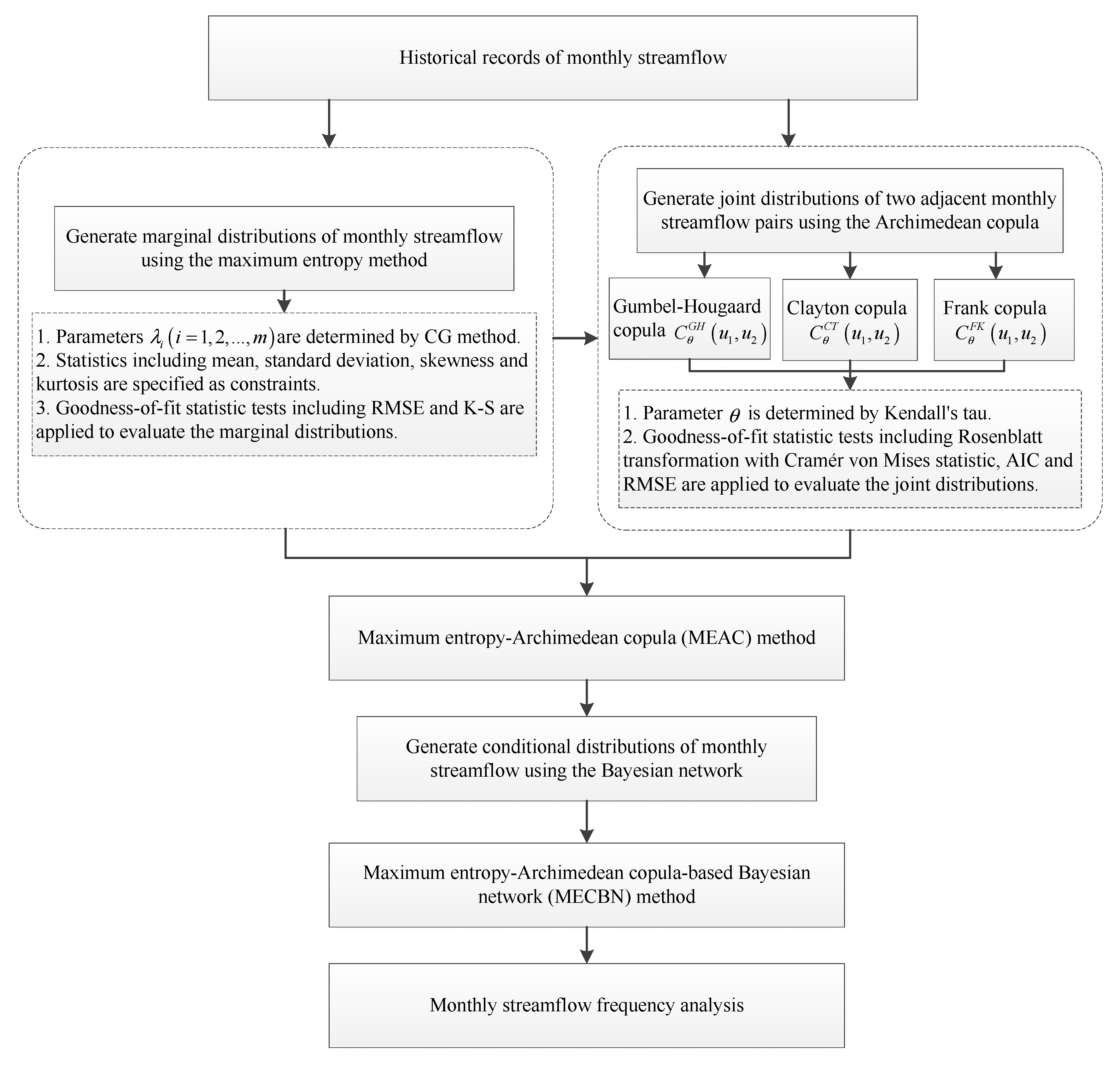
2.3. Maximum Entropy-Archimedean Copula Method

A maximum entropy-Archimedean copula (MEAC) method can be proposed through integrating techniques of maximum entropy and Archimedean copula into a general framework. In MEAC, the marginal distribution of monthly streamflow is constructed by the maximum entropy method and the joint distribution of two adjacent monthly streamflows is constructed by an Archimedean copula. The joint distribution of the MEAC method can be formulated as follows:
P ( X x , Y y ) = C θ ( u 1 , u 2 ) = C θ ( F X ( x ; λ ) , F Y ( y ; λ ) )
F X ( x ; λ ) = a 1 x exp [ ln ( a 1 b 1 exp ( i = 1 m λ i h i ( x ) ) d x ) i = 1 m λ i h i ( x ) ] d t
F Y ( y ; λ ) = a 2 y exp [ ln ( a 2 b 2 exp ( i = 1 m λ i h i ( y ) ) d y ) i = 1 m λ i h i ( y ) ] d t
where C θ ( u 1 , u 2 ) is the Archimedean copula with parameter θ ; u 1 = F X ( x ; λ ) and u 2 = F Y ( y ; λ ) are the marginal distributions of random variables X and Y , respectively. h i ( x ) and h i ( y ) are known functions of X and Y ; a 1 and b 1 are the lower and upper bounds of the random variable X , respectively; a 2 and b 2 are the lower and upper bounds of random variable Y , respectively; λ i ( i = 1 , 2 , , m ) and λ i ( i = 1 , 2 , , m ) are the Lagrange multipliers. The parameters of MEAC could be estimated by the inference functions for margins (IFM) method [31]. The parameter of the Archimedean copula could be estimated by Kendall’s tau. The CG method could be used for the parameter estimation of marginal distribution.

2.4. Maximum Entropy-Archimedean Copula-Based Bayesian Network

Based on the MEAC method, the joint distribution of adjacent monthly streamflows could be generated. However, the frequency analysis of monthly streamflow also needs to construct the conditional dependency of adjacent monthly streamflows. Therefore, a Bayesian network is introduced in this study in order to obtain the conditional dependencies of monthly streamflow. As a probabilistic model, a Bayesian network can describe the conditional dependencies of a set of random variables via directed acyclic graphs [29,30]. The joint PDF of different random variables with a level of dependency ( x t 1 , x t 2 , , x t n ) within a Bayesian network can be defined as follows [30]:
f ( x t 1 , x t 2 , , x t p ) = t j T f ( x t j | x t 1 , , x t j 1 )
Based on Equation (10), the expression of conditional PDF of two adjacent monthly streamflows, X and Y , can be described as follows:
f ( y | x ) = f ( x , y ) f X ( x ) = c θ ( u 1 , u 2 ) f X ( x ) f Y ( y ) f X ( x ) = c θ ( u 1 , u 2 ) f Y ( y )
where c θ ( u 1 , u 2 ) is the PDF of the Archimedean copula with parameter θ , which describes the joint PDF of two adjacent monthly streamflows; u 1 = F X ( x ; λ ) and u 2 = F Y ( y ; λ ) are the marginal distributions of monthly streamflows whose marginal PDFs are f X ( x ) and f Y ( y ) , respectively. The PDF of copula c θ ( u 1 , u 2 ) can be defined as follows:
c θ ( u 1 , u 2 ) = C θ ( u 1 , u 2 ) u 1 , u 2 = C θ ( F X ( x ; λ ) , F Y ( y ; λ ) ) u 1 , u 2
The general framework of MECBN for modeling hydrological processes is shown in Figure 1. The MECBN method would be used for monthly streamflow frequency analysis. The application involves the construction of marginal, joint and conditional distributions, and the measurement of dependence. In detail, (a) the marginal distributions of monthly streamflows would be constructed by the maximum entropy method; (b) the joint distributions of two adjacent monthly streamflows would be estimated using Archimedean copula based on the generated marginal distributions; (c) the performance of marginal and joint distributions would be tested by the goodness-of-fit statistics; (d) the conditional distributions of two adjacent monthly streamflows would be generated by the Bayesian network combined with generated marginal and joint distributions; (d) the dependence between two adjacent monthly streamflows would be measured by methods including Spearman’s rho, Kendall’s tau and the tail dependence coefficient.

3. Study Area and Measures
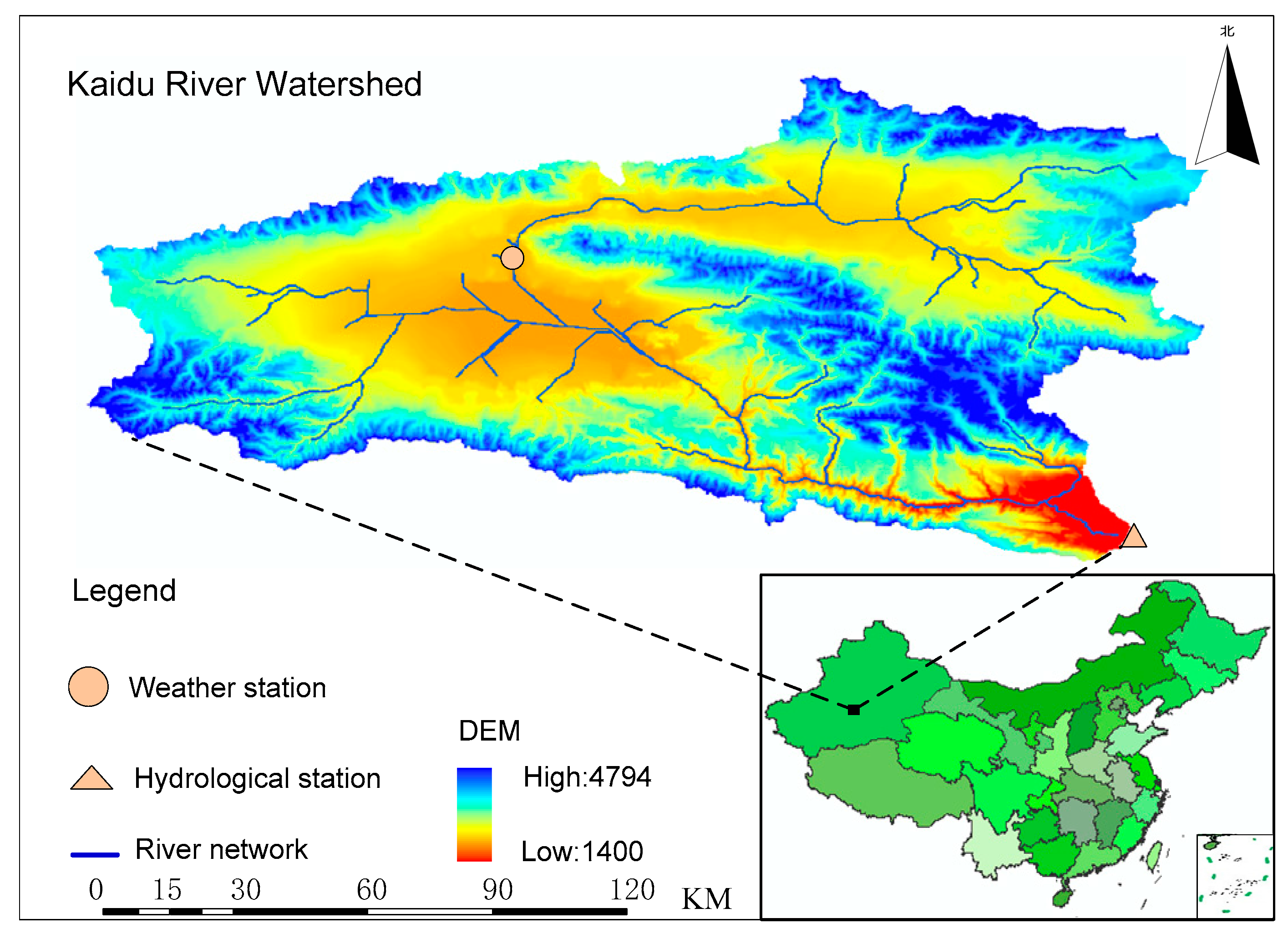
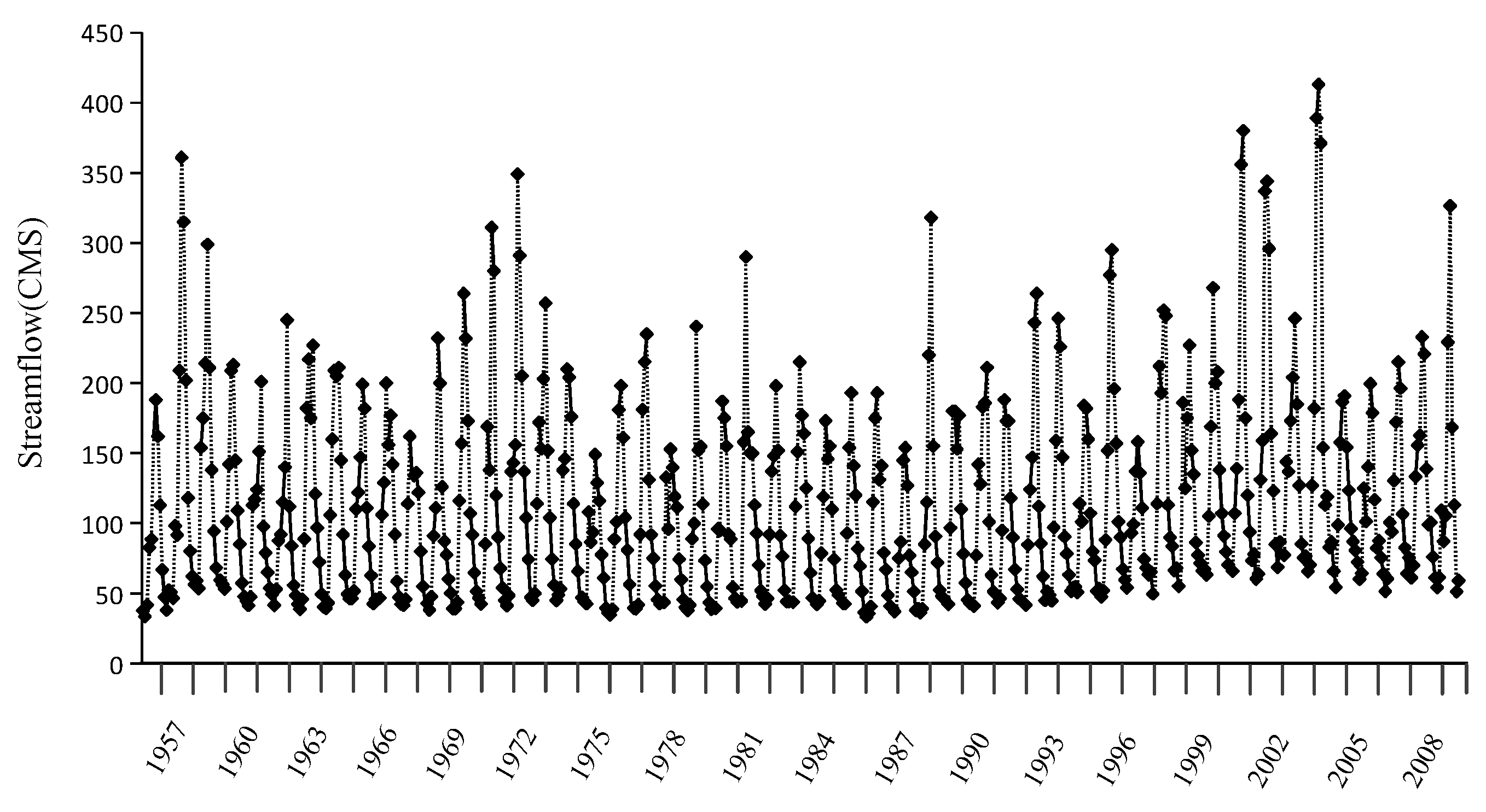
3.1. Study Area

The Kaidu River Basin (Figure 2), located in the middle reach of the Tarim River Basin, plays a key role in water supply to municipality, industry, agricultural, stockbreeding and forestry sectors in Xinjiang province of China. It lies between the latitudes of 42°14′ N and 43°21′ N and longitudes of 82°58′ E and 86°05′ E [36]. The Kaidu River Basin experiences a typical inner-continental climate, with an average annual temperature of 4.16 °C. The spatial and temporal distribution of precipitation in the Kaidu River Basin is heterogeneous with an average rainfall of 273 mm/year Huang et al. [37]. It exhibits plentiful snowmelt water in spring, concentrated ice-melt water and rainfall recharge during the summer, significant temperature differences during the autumn, and frequent early frost in winter. More than 80% of the rainfall occurs between May and September [38]. The study site is Dashankou hydrological station, which is located at the Kaidu River Basin outlet. The Kaidu River Basin above Dashankou hydrological station has a catchment area of 18,827 km2 with the mean elevation of 3100 m. The data of streamflow records are obtained from the Dashankou hydrological station for the period of 1957–2009. The unit for streamflow is in cubic meter per second (CMS). The monthly variation of streamflow is shown in Figure 3, with a maximum value of 413, a minimum value of 33.2, a mean of 110.54, a standard deviation of 68.77, a skewness of 1.37, and a kurtosis of 5.07.
The Kaidu River Basin has important functions for agricultural irrigation and ecological sustainability. It also plays a critical role in protecting the Bosten Lake. However, the regional water-resources systems have been destroyed because of excessive exploitation and environmental degradation, leading to amounts of ecological and environmental problems. Moreover, the streamflow is replenished by snowmelt in spring, sometimes causing floods. Therefore, it is necessary to propose an effective method to analyze the inherent uncertain characteristics on streamflow of the Kaidu River Basin. In this paper, potential streamflow interactions are explored and formalized into a copula function combined with a Bayesian network framework. An application using such frequency analysis method could be developed as part of a strategy for water resources management and precaution of hydrological extremes.

3.2. Dependence Measures

In streamflow analysis, one may be interested in dependence structure between adjacent streamflows, especially for the extreme behavior of the streamflows for risk analysis. Therefore, the rank-based coefficients of correlation including Spearman’s rho and Kendall’s tau, which are well-known non-parametric measures of dependence, are applied to examine the dependence structure of adjacent monthly streamflows. The tail dependence coefficient is used to analyze the extreme behavior of adjacent monthly streamflows [39]. The simplification of Spearman’s rho can be expressed as:
ρ ^ s = 1 6 n ( n 2 1 ) i = 1 n ( R i Q i ) 2
where ρ ^ s [ 1 , 1 ] , ( X i , Y i ) ,   i = 1 , 2 , , n are the sample of ( X , Y ) ; R i stands for the rank of X i among ( X 1 , X 2 , , X n ) , and Q i stands for the rank of Y i among ( Y 1 , Y 2 , , Y n ) . For Kendall’s tau, it can be expressed as:
τ ^ = c d c + d = c d C n 2
where c and d are the number of concordant of discordant pairs, respectively; ( X i , Y i ) and ( X j , Y j ) are said to be concordant when ( X i X j ) ( X i Y j ) > 0 and discordant when ( X i X j ) ( X i Y j ) < 0 . The lower and upper tail dependence coefficients are introduced as follows:
λ l o = lim P [ Y < G 1 ( u ) | X < F 1 ( u ) ]
λ u p = lim P [ Y > G 1 ( u ) | X > F 1 ( u ) ]
where λ l o and λ u p are the lower and upper dependence coefficients, respectively; F ( x ) and G ( x ) are the marginal distributions of random variable X and Y , respectively.

3.3. Goodness-of-Fit (GOF)

The goodness-of-fit (GOF) statistic tests for marginal and joint distributions can be performed separately. In this study, the GOF tests for marginal distributions include the root mean square error (RMSE) and the Kolmogorov–Smirnov (K–S) test. The GOF tests for joint distributions consist of the Rosenblatt transformation with Cramér von Mises statistic, the Akaike information criterion (AIC), and RMSE. The expression of RMSE is Willmott and Matsuura [40]:
R M S E = k = 1 N ( x k e s t x k o b s ) 2 N
where x k e s t is the estimated value from the fitted distribution; x k o b s is the corresponding observed value; N is the sample size.
As a non-parametric probability distribution free test, the K–S test quantifies the largest vertical difference between the specified and empirical distributions. The statistic of the K–S test is defined as follows:
T = sup x | F ( x ) F n ( x ) |
where data points x are in an increasing order; F ( x ) and F n ( x ) are the specified distribution and empirical distribution, respectively; If T exceeds the 1 α quantile, then we reject the null hypothesis H 0 (The sample data follow the hypothesized distribution); α is the level of significance.
The GOF tests based on the Rosenblatt transformation with Cramér von Mises statistic, Akaike information criterion (AIC) and RMSE are employed in this study. The empirical distribution for the Rosenblatt transformation and the corresponding Cramér von Mises statistic can be expressed as follows [31]:
D n ( υ ) = 1 n i = 1 n 1 ( E i υ ) , υ [ 0 , 1 ]
S n ( B ) = n 0 1 { D n ( υ ) C ( υ ) } 2 d υ = n 3 2 1 2 i = 1 n ( 1 E i 1 2 ) ( 1 E i 2 2 ) + 1 n i = 1 n j = 1 n ( 1 E i 1 E j 1 ) ( 1 E i 2 E j 2 )
where E i stand for the pseudo-observations from the independence copula C ; υ is the vector of marginal distributions; n is the sample size; E i l E j l = max ( E i l , E j l ) , ( l = 1 , 2 ) . The corresponding p-value of the Cramér von Mises test statistic exceeds the 1 α quantile, then we reject the null hypothesis H 0 (the hypothesized copula function is the fitted one); α is the level of significance. Then, AIC can be used for identifying the most appropriate probability distribution, which can be expressed below:
AIC = N log [ 1 N k = 1 N ( x k e s t x k o b s ) 2 ] + 2 ( n o .   o f   f i t t e d   p a r a m e t e r s )
The RMSE value for joint distribution can also be determined using Equation (17). The best fitted copula function is the one that has the minimum values of AIC and RMSE.

4. Results and Discussion

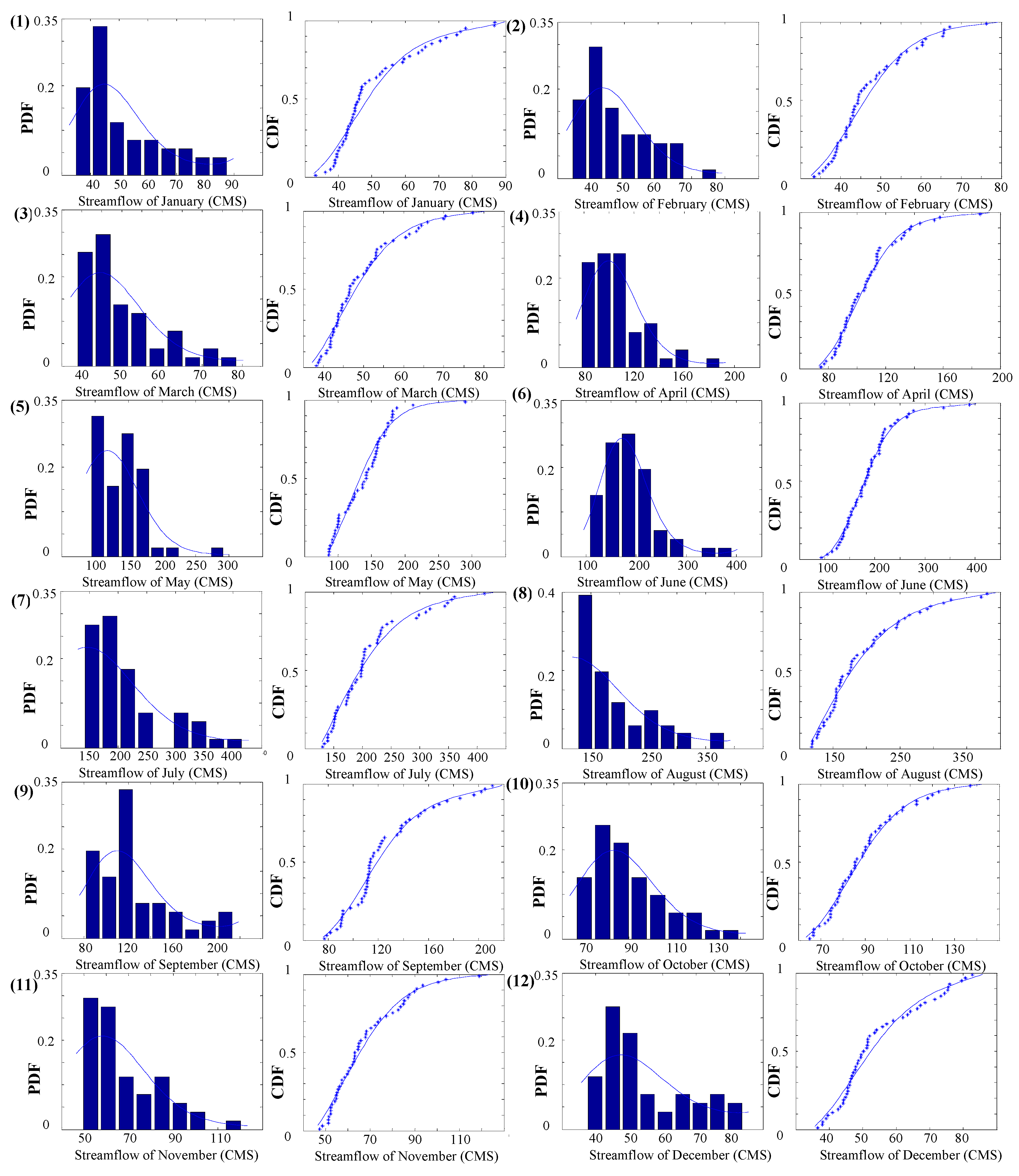
4.1. Marginal Distributions

Firstly, marginal distributions of monthly streamflows are constructed. The Lagrange multipliers for the marginal distributions are estimated by the CG method. The results of estimation are shown in Table 1. Based on the Lagrange multipliers, the PDFs and CDFs of monthly streamflows in the Kaidu River Basin could be determined based on Equations (6) and (7). In order to evaluate the marginal distributions of monthly streamflow in Kaidu River Basin generated by the MECBN method, GOF tests including RMSE and K–S test are applied in this study. The results are shown in Table 2.
As a measure which is regularly employed in model evaluation studies, RMSE indicates the deviation between generated monthly streamflow and observed monthly streamflow. Most RMSE values in Table 2 are small. The maximum value of RMSE is 10.28. This means that the maximum deviation between generated monthly streamflow and observed monthly streamflow occurs in July, while the minimum RMSE can be observed in March with a value of 1.20. The K–S test can quantify the largest vertical difference between the hypothesized and empirical distributions [31,41,42]. Therefore, it can be used to verify if the sample data of monthly streamflow follow the marginal distribution generated by the MECBN method. As presented in Table 2, all the p-Values calculated from K–S test are higher than the significant level α = 0.05, where T is the K–S test statistic. The results indicate that observed monthly streamflows in the Kaidu River Basin could be appropriately represented by the marginal distributions generated by MECBN.
Figure 4 shows the comparison of theoretial and empirical marginal PDF and CDF for monthly streamflow in Kaidu River Basin. Numbers (1) to (12) stand for monthly streamflow from January to December. It could be concluded that the marginal PDF and CDF generated by MECBN are able to capture the shape of empirical histograms and empirical CDF. Therefore, MECBN is effective for generating marginal distributions of monthly streamflows of the Kaidu River Basin. In addition, Figure 4 indicates that most streamflow records in April, May, June, July, August and September are greater than 100 CMS. The streamflow values from April to September, corresponding to the 0.5 value of CDF, are greater than 100 CMS. That is mainly because the distribution of precipitation is uneven in Kaidu River Basin. More than 80% of the total precipitation in a year falls from May to September, and the rest falls from October to April. However, there is a low rainfall but a high streamflow in April. This is due to the fact that snow melting is the main sources in April in the Kaidu River Basin.

4.2. Joint Distributions

In this study, Archimedean copulas including Gumbel–Hougaard, Clayton and Frank copulas would be used to generate the joint probability distributions for adjacent monthly streamflows. In order to evaluate the joint distributions generated by MECBN, the GOF tests of the Rosenblatt transformation with the Cramér von Mises statistic, AIC and RMSE would be employed. As shown in Table 3. All the p-Values of adjacent monthly streamflow pairs are higher than significant level α = 0.05 for the Gumbel–Hougaard and Frank copulas. When employing Clayton copula to generate joint distributions, the p-Values of months 4–5, 6–7 and 9–10 are lower than the significant level. Results in Table 3 mean that both Gumbel–Hougaard and Frank copulas could be used to generate joint distributions of two adjacent monthly streamflows. In order to choose the most appropriate copula for monthly streamflow pairs in the Kaidu River Basin, the AIC and RMSE values are applied to test goodness of fitness for sample data to the joint distribution obtained by the Gumbel–Hougaard and Frank copulas. Results are given in Table 4. The Gumbel–Hougaard copula would be chosen as the most appropriate copula with the minimum values of AIC and RMSE for monthly streamflow pairs.
Based on the analysis above, marginal distributions of monthly streamflow were generated and the Gumbel–Hougaard copula was chosen to describe the dependence structures for adjacent monthly streamflows in the Kaidu River Basin. Therefore, joint PDF, joint CDF and the corresponding counters are obtained by the MECBN method. Dependence measures (i.e., Table 5) indicate that the adjacent monthly streamflow pairs in the Kaidu River Basin are highly correlated with significant upper tail dependence. The upper tail dependence between two adjacent monthly streamflows indicates that streamflow of one month in the Kaidu River Basin depends on the streamflow of its adjacent month, and also denotes the probability for one monthly streamflow exceeding a high threshold under the situation that its adjacent monthly streamflow exceeds that threshold. It is important to determine this in order to provide vital information for the prevention and control of hydrological extremes in the Kaidu River Basin.

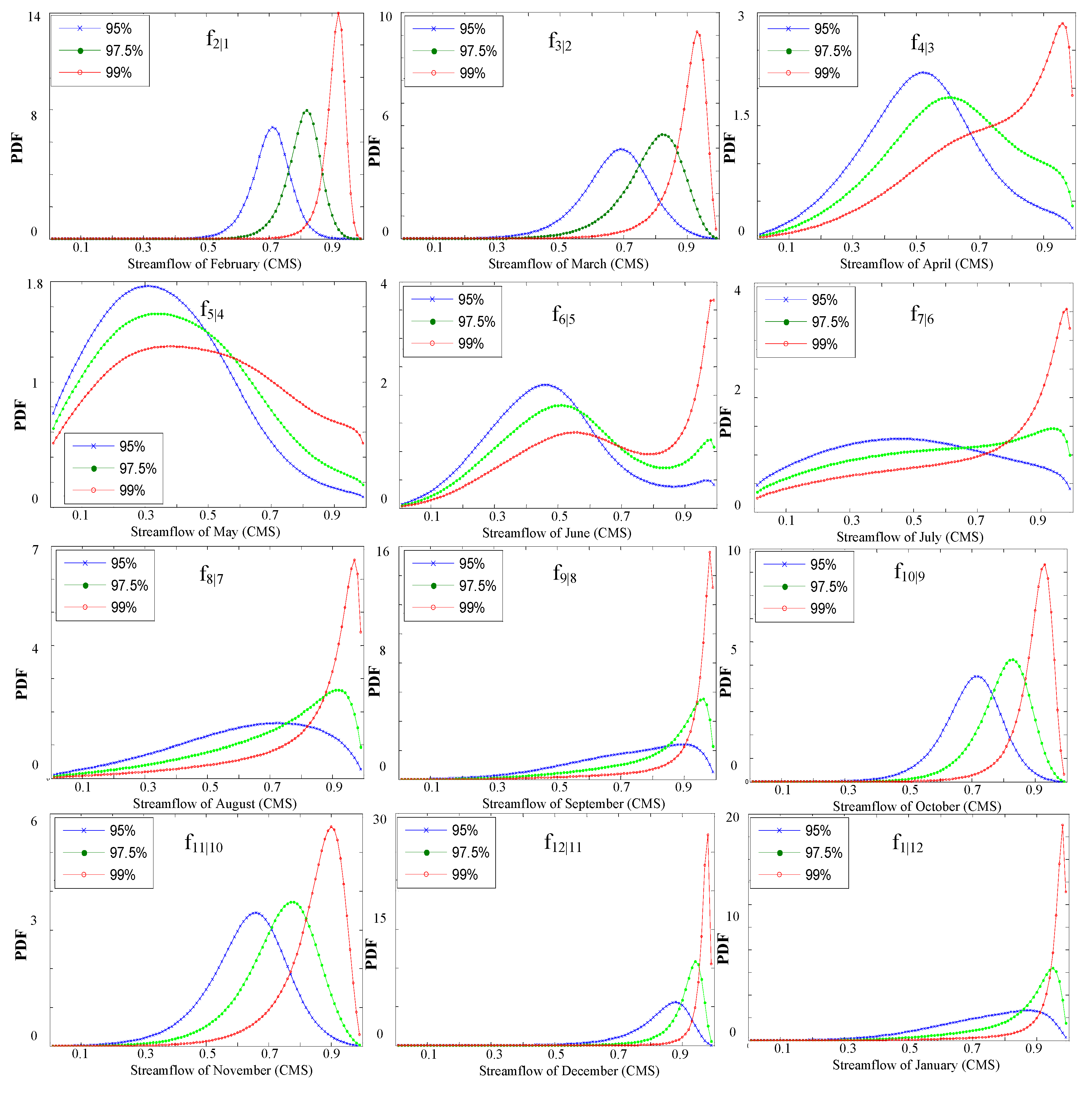
4.3. Conditional Distributions

Once the marginal and joint distributions are fitted to streamflow records in the Kaidu River Basin, the conditional distributions of adjacent monthly streamflows can be derived according to Equation (11). The streamflow status is classified based on the quantile. In this study, 95, 97.5 and 99 percentile values reflect qualitative information on probability distributions of the scaled monthly streamflow of the Kaidu River Basin. They are used as streamflow classification schemes at high level to explore the conditional distribution. As the streamflow has been scaled into [0,1], 95% means that the streamflow is 0.95. The relationship of conditional distribution of two adjacent months has been transformed to the exploration of the distribution of the streamflow in each month given the streamflow status (0.95, 0.975, 0.99) in the last month demonstrated in Figure 5.
As shown in Figure 5, if the given streamflow percentile value changes in the previous, the probability distribution of the streamflow in the current month varies, which also exhibits the conclusion that there exists upper tail dependence between every two adjacent monthly streamflows in the Kaidu River Basin. Moreover, the probability distributions under a given streamflow percentile value, and the fluctuation ranges under different streamflow percentile values vary considerably between different streamflow pairs. It indicates that the upper tail dependences between each streamflow pairs are different, which are coincide to the upper tail coefficients presented in Table 5. It is also interesting to find that the dependence coefficients including Spearman’s rho, Kendall’s tau and upper tail dependence coefficients are in inverse proportion to monthly streamflow values in the Kaidu River Basin. In detail, the streamflows in April, May, June, August and September are higher than those in other months. But the dependence coefficients between March and April, April and May, May and June, June and August, and August and September are lower than other monthly streamflow pairs. Among all the streamflow pairs, the dependence between January and February is most significant with the values of Spearman’s rho, Kendall’s tau and upper tail dependence coefficient being 0.931, 0.784, and 0.838, respectively. It leads to the results that the streamflow in February depends significantly on the streamflow in January and the PDF of streamflow in February varies greatly along with the changes of streamflow status in January. The minimum values of Spearman’s rho, Kendall’s tau and upper tail dependence coefficient are 0.292, 0.180 and 0.235, respectively. They reveal the interaction of monthly streamflows between April and May. Obviously, f5|4 indicates the small change of PDF for streamflow in May when the scaled streamflow of April changes from 0.95 to 0.99. These results show that: (a) in general, high magnitudes of two adjacent streamflow corresponds to a low dependence coefficient among them, and vice versa; (b) the two minimum adjacent streamflows exhibit the highest dependence, but the two maximum streamflows do not show the minimum dependent coefficent, which indicates the interaction between streamflow and dependence coefficient is non-linear. That is mainly because (a) there are a variety of factors which affect the streamflow in the Kaidu River Basin, such as rainfall, snow melting, evapotranspiration rate, requirement of water use, and so on; (b) the conditions of streamflow are more complex under flooding season in the Kaidu River Basin, which leads to the situation that months with high streamflow values under flooding season have weak correlations with their adjacent months. In addition, the dependence coefficient between April and May is minimum mainly due to the types of streamflow contributors being different in April and May. It has been concluded before that snow melting is the main source in April in the Kaidu River Basin. However, both rainfall and snow melting make major contributions to the runoff in May. Otherwise, the conditions that the evapotranspiration rate increases with increasing temperature and the requirement of water increases due to the growth of the plants and the impact of human use may also affect the interaction of streamflow pairs between April and May.

5. Conclusions

In this study, a maximum entropy-Archimedean copula-based Bayesian network (MECBN) method has been developed in order to analyze the interaction of monthly streamflows. MECBN is effective for representing the uncertainties existing in the model representation, preserving the distributional characteristics of streamflow records and addressing the correlation structure between streamflow pairs. This study is the first attempt at introducing a maximum entropy-copula into the Bayesian network modeling framework. Compared to the conventional Bayesian network approach, MECBN is more effective for addressing the correlation structure between streamflow pairs with arbitrary random characteristics. Moreover, the marginal distribution of monthly streamflow is approximated by the maximum entropy method. Such a method could preserve key statistics, and does not require specific assumptions (e.g., normal, gamma etc.) on the historical streamflow data. The limitations of MECBN is that the selection of copula functions needs more computation to ensure the validity of preserving the non-linear dependence structure. Moreover, the determination of parameters in the MECBN method is computationally cumbersome.
The proposed method has been applied to frequency analysis of monthly streamflow in Kaidu River Basin. The results indicate that (a) MECBN can preserve the key statistical characteristics (i.e., mean, standard deviation, skewness and kurtosis) for each monthly streamflow in the Kaidu River Basin; (b) the Gumbel–Hougaard copula among Archimedean copulas is the most appropriate for reflecting the interactions of monthly streamflow pairs, with the minimum values of AIC and RMSE; (c) the joint distributions, the conditional distributions and the dependence measures including Spearman’s Rho, Kendall’s Tau and the tail dependence coefficient reveal the upper tail dependence between monthly streamflow pairs in the Kaidu River Basin; (d) the goodness-of-fit statistical tests show a good performance of MECBN in describing the historical data of the Kaidu River Basin, China.
The frequency analysis of monthly streamflow in the Kaidu River Basin indicates that the interactions between two adjacent monthly streamflow pairs are non-linear. Compared with the other months, there is a low rainfall but a high streamflow in April due to the fact that snow melting is the main source for the streamflow in April in the Kaidu River Basin. The upper tail dependence between monthly streamflow pairs in the Kaidu River Basin indicates that streamflow of one month depends on the streamflow of its adjacent month. It also denotes a high probability for one monthly streamflow exceeding a high threshold under the situation that its adjacent monthly streamflow exceeds the threshold. The upper tail dependence varies from different streamflow status (95%, 97.5% and 99% quantiles of streamflow) and is described by the upper tail dependence coefficients. The dependence coefficients of Spearman’s rho, Kendall’s tau and the upper tail dependence coefficient are in inverse proportion to monthly streamflow values in the Kaidu River Basin. This is because a variety of factors (i.e., rainfall, snow melting, evapotranspiration rate and requirement of water use) would affect the streamflow in the Kaidu River Basin in the flooding season, leading to less impact from the streamflow in the antecedent month. These findings have great significance for the Kaidu River Basin, which is located in the arid region of China. They can be used for providing vital information for the prevention and control of hydrological extremes and further water resources planning in the Kaidu River Basin.

Author Contributions

Methodology and Writing-Original Draft, X.K.; Software and Modelling calculation, X.Z. and C.C.; Formal Analysis and Validation, Y.F.; Resources and Data Curation, G.H. and Y.L.; Writing-Review & Editing, C.W.

Funding

This research was funded by [the Training Programme Foundation for the Beijing Municipal Excellent Talents] grant number [2017000020124G179], [National Sciences Foundation] grant number [51520105013, 51679087], [National Natural Science Foundation of China] grant number [41701621], [the 111 Program] grant number [B14008].

Acknowledgments

The authors are grateful to the editors and the anonymous reviewers for their insightful comments and suggestions.

Conflicts of Interest

The authors declare no conflict of interest.

References

  1. Hu, Q.; Huang, G.H.; Liu, Z.F.; Fan, Y.R.; Li, W. Inexact fuzzy two-stage programming for water resources management in an environment of fuzziness and randomness. Stoch. Environ. Res. Risk Assess. 2012, 26, 261–280. [Google Scholar] [CrossRef]
  2. Huang, G.H.; Cohen, S.J.; Yin, Y.Y.; Bass, B. Incorporation of inexact dynamic optimization with fuzzy relation analysis for integrated climate change impact study. J. Environ. Manag. 1996, 48, 45–68. [Google Scholar] [CrossRef]
  3. Cheng, G.H.; Huang, G.H.; Dong, C.; Baetz, B.W.; Li, Y.P. Interval recourse linear programming for resources and environmental systems management under uncertainty. J. Environ. Inform. 2017, 30, 119–136. [Google Scholar] [CrossRef]
  4. Huang, Y.; Qin, X.S. A pseudospectral collocation approach for flood inundation modelling with random input fields. J. Environ. Inform. 2017, 30, 95–106. [Google Scholar] [CrossRef]
  5. Li, Y.P.; Huang, G.H.; Nie, S.L.; Liu, L. Inexact multistage stochastic integer programming for water resources management under uncertainty. J. Environ. Manag. 2008, 88, 93–107. [Google Scholar] [CrossRef] [PubMed]
  6. Fan, Y.R.; Huang, G.H.; Baetz, B.W.; Li, Y.P.; Huang, K. Development of a copula-based particle filter (CopPF) approach for hydrologic data assimilation under consideration of parameter interdependence. Water Resour. Res. 2017, 53, 4850–4875. [Google Scholar] [CrossRef]
  7. Fan, Y.R.; Huang, W.W.; Huang, G.H.; Huang, K.; Zhou, X. A PCM-based stochastic hydrological model for uncertainty quantification in watershed systems. Stoch. Environ. Res. Risk Assess. 2015, 29, 915–927. [Google Scholar] [CrossRef]
  8. Chen, B.; Li, P.; Wu, H.J.; Husain, T.; Khan, F. MCFP: A monte carlo simulation-based fuzzy programming approach for optimization under dual uncertainties of possibility and continuous probability. J. Environ. Inform. 2017, 29, 88–97. [Google Scholar] [CrossRef]
  9. Han, J.C.; Huang, G.H.; Zhang, H.; Li, Z.; Li, Y.P. Bayesian uncertainty analysis in hydrological modeling associated with watershed subdivision level: A case study of SLURP model applied to the Xiangxi River watershed, China. Stoch. Environ. Res. Risk Assess. 2014, 28, 973–989. [Google Scholar] [CrossRef]
  10. Pastori, M.; Udías, A.; Bouraoui, F.; Bidoglio, G. A multi-objective approach to evaluate the economic and environmental impacts of alternative water and nutrient management strategies in Africa. J. Environ. Inform. 2017, 29, 16–28. [Google Scholar] [CrossRef]
  11. Jordan, Y.C.; Ghulam, A.; Chu, M.L. Assessing the impacts of future urban development patterns and climate changes on total suspended sediment loading in surface waters using Geoinformatics. J. Environ. Inform. 2014, 24, 65–79. [Google Scholar] [CrossRef]
  12. Li, Z.; Huang, G.H.; Fan, Y.R.; Xu, J.L. Hydrologic Risk Analysis for Nonstationary Streamflow Records under Uncertainty. J. Environ. Inform. 2016, 26, 41–51. [Google Scholar]
  13. Kong, X.M.; Huang, G.H.; Li, Y.P.; Fan, Y.R.; Zeng, X.T.; Zhu, Y. Inexact copula-based stochastic programming method for water resources management under multiple uncertainties. J. Water Resour. Plan. Manag. 2018, 144, 04018069. [Google Scholar] [CrossRef]
  14. Fan, Y.R.; Huang, G.H.; Zhang, Y.; Li, Y.P. Uncertainty quantification for multivariate eco-hydrological risk in the Xiangxi River within the Three Gorges Reservoir Area in China. Engineering 2018, 4, 617–626. [Google Scholar] [CrossRef]
  15. Fan, Y.R.; Huang, W.W.; Huang, G.H.; Huang, K.; Li, Y.P.; Kong, X.M. Bivariate hydrologic risk analysis based on a coupled entropy-copula method for the Xiangxi River in the Three Gorges Reservoir area, China. Theor. Appl. Climatol. 2016, 125, 381–397. [Google Scholar] [CrossRef]
  16. Fan, Y.R.; Huang, W.W.; Huang, G.H.; Li, Y.P.; Huang, K.; Li, Z. Hydrologic risk analysis in the Yangtze River basin through coupling Gaussian mixtures into copulas. Adv. Water Resour. 2016, 88, 170–185. [Google Scholar] [CrossRef]
  17. Asztalos, J.R.; Kim, Y. Lab-Scale Experiment and model study on enhanced digestion of wastewater sludge using bioelectrochemical systems. J. Environ. Inform. 2017, 29, 98–109. [Google Scholar] [CrossRef]
  18. Kong, X.M.; Huang, G.H.; Fan, Y.R.; Li, Y.P.; Zeng, X.T.; Zhu, Y. Risk analysis for water resources management under dual uncertainties through factorial analysis and fuzzy random value-at-risk. Stoch. Environ. Res. Risk Assess. 2017, 31, 1–16. [Google Scholar] [CrossRef]
  19. Kong, X.M.; Huang, G.H.; Fan, Y.R.; Li, Y.P. A duality theorem-based algorithm for inexact quadratic programming problems: Application to waste management under uncertainty. Eng. Optim. 2016, 48, 562–581. [Google Scholar] [CrossRef]
  20. Lima, C.H.R.; Lall, U. Spatial scaling in a changing climate: A hierarchical Bayesian model for non-stationary multi-site annual maximum and monthly streamflow. J. Hydrol. 2010, 383, 307–318. [Google Scholar] [CrossRef]
  21. Erro, J.; Lόpez, J.J. Regional frequency analysis of annual maximum streamflow in Gipuzkoa (Spain). Geophys. Res. Abstr. 2012, 14, 8274. [Google Scholar]
  22. Schnier, S.; Cai, X.M. Prediction of regional streamflow frequency using model tree ensembles. J. Hydrol. 2014, 517, 298–309. [Google Scholar] [CrossRef]
  23. Zhang, Q.; Gu, X.H.; Singh, V.P.; Xiao, M.Z.; Xu, C.Y. Flood frequency under the influence of trends in the Pearl River basin, China: Changing patterns, causes and implications. Hydrol. Process. 2015, 29, 1406–1417. [Google Scholar] [CrossRef]
  24. Chan, T.U.; Hart, B.T.; Kennard, M.J.; Pusey, B.J.; Shenton, W.; Douglas, M.M.; Valentine, E.; Patel, S. Bayesian network models for environmental flow decision making in the Daly River, Northern Territory, Australia. River Res. Appl. 2012, 28, 283–301. [Google Scholar] [CrossRef]
  25. Nagarajan, K.; Krekeler, C.; Slatton, K.C.; Graham, W.D. A scalable approach to fusing spatiotemporal data to estimate streamflow via a Bayesian network. IEEE Trans. Geosci. Remote Sens. 2010, 48, 3720–3732. [Google Scholar] [CrossRef]
  26. Mediero, L.; Santillán, D.; Garrote, L. Flood quantile estimation at ungauged sites by Bayesian networks. Geophys. Res. Abstr. 2012, 14, 11998. [Google Scholar]
  27. Zhang, D.; Yan, X.P.; Yang, Z.L.; Wall, A.; Wang, J. Incorporation of formal safety assessment and Bayesian network in navigational risk estimation of the Yangtze River. Reliab. Eng. Syst. Saf. 2013, 118, 93–105. [Google Scholar] [CrossRef]
  28. D’Addabbo, A.; Refice, A.; Pasquariello, G. A Bayesian network approach to perform SAR/InSAR data fusion in a flood detection problem. Proc. SPIE 2014, 9224, 9244. [Google Scholar]
  29. Madadgar, S.; Moradkhani, H. A Bayesian framework for probabilistic seasonal drought forecasting. J. Hydrometeorol. 2013, 14, 1685. [Google Scholar] [CrossRef]
  30. Madadgar, S.; Moradkhani, H. Spatio-temporal drought forecasting within Bayesian networks. J. Hydrol. 2014, 512, 134–146. [Google Scholar] [CrossRef]
  31. Kong, X.M.; Huang, G.H.; Fan, Y.R.; Li, Y.P. Maximum entropy-Gumbel-Hougaard copula method for simulation of monthly streamflow in Xiangxi River, China. Stoch. Environ. Res. Risk Assess. 2015, 29, 833–846. [Google Scholar] [CrossRef]
  32. Hao, Z.; Singh, V.P. Entropy-based parameter estimation for extended three-parameter Burr III distribution for low-flow frequency analysis. Trans. ASABE 2009, 52, 1193–1202. [Google Scholar] [CrossRef]
  33. Genest, C.; Favre, A.C. Everything you always wanted to know about copula modeling but were afraid to ask. J. Hydrol. Eng. 2007, 12, 347–368. [Google Scholar] [CrossRef]
  34. Genest, C.; MacKay, J. The joy of copulas: Bivariate distributions with uniform marginal (Com: 87V41 P248). Am. Stat. 1986, 40, 280–283. [Google Scholar]
  35. Nelsen, R.B. An Introduction to Copulas; Springer: New York, NY, USA, 1999. [Google Scholar]
  36. Wang, C.X.; Li, Y.P.; Zhang, J.L.; Huang, G.H. Assessing parameter uncertainty in semi-distributed hydrological model based on type-2 fuzzy analysis—A case study of Kaidu River. Hydrol. Res. 2015. [Google Scholar] [CrossRef]
  37. Huang, Y.; Chen, X.; Li, Y.P.; Huang, G.H.; Liu, T. A fuzzy-based simulation method for modelling hydrological processes under uncertainty. Hydrol. Process. 2010, 24, 3718–3732. [Google Scholar] [CrossRef]
  38. Fu, A.H.; Chen, Y.N.; Li, W.H.; Li, B.F.; Yang, Y.H.; Zhang, S.H. Spatial and temporal patterns of climate variations in the Kaidu River Basin of Xinjiang, Northwest China. Quat. Int. 2013, 311, 117–122. [Google Scholar] [CrossRef]
  39. Poulin, A.; Huard, D.; Favre, A.C.; Pugin, S. Importance of tail dependence in bivariate frequency analysis. J. Hydrol. Eng. 2007, 12, 394–403. [Google Scholar] [CrossRef]
  40. Willmott, C.J.; Matsuura, K. Advantages of the Mean Absolute Error (MAE) over the Root Mean Square Error (RMSE) in assessing average model performance. Clim. Res. 2005, 30, 79–82. [Google Scholar] [CrossRef]
  41. Massey, F.J. The Kolmogorov-Smirnov test for goodness of fit. J. Am. Stat. Assoc. 1951, 46, 68–78. [Google Scholar] [CrossRef]
  42. Razali, N.M.; Wah, Y.B. Power comparisions of Shapiro-Wilk, Kolmogorov-Smirnov, Lilliefors and Anderson-Darling tests. J. Stat. Model. Anal. 2011, 2, 21–33. [Google Scholar]
Figure 1. General framework of the maximum entropy-Archimedean copula-based Bayesian network (MECBN).
Water 11 00042 g001
Figure 2. The Kaidu River Basin.
Water 11 00042 g002
Figure 3. Trend of monthly streamflow from 1957 to 2009.
Water 11 00042 g003
Figure 4. Comparison of theoretical and empirical marginal probability density function (PDF) and cumulative density function (CDF). The values are calculated monthly from 1957 to 2009. The abscissa represents streamflow values. The corresponding size varies from month to month. PDF describes the output of variables, and indicates the frequency at a given streamflow value. CDF describes the integrate of PDF, and indicates the probability of a given streamflow value. Lines in PDFs and CDFs show the performance of generated values. Bars and dots depict the empirical values in PDFs and CDFs, respectively.
Water 11 00042 g004
Figure 5. Distribution of streamflow in each month given the streamflow status (0.95, 0.975, 0.99) in the previous month. The values are calculated monthly from 1957 to 2009. The abscissa represents streamflow values, which are scaled into [0,1]. fK+1|K indicates the conditional PDF of two adjacent monthly streamflows, K and K+1. 0.95, 0.975 and 0.99 mean the steamflow status of K’s streamflow.
Water 11 00042 g005
Table 1. Estimation of Lagrange multipliers for maximum entropy (ME)-based marginal distribution of monthly streamflow.
Month λ 1 λ 2 λ 3 λ 4
1−6.7816.35−1.14−7.60
2−6.3413.510.39−5.47
3−4.2712.13−0.62−4.89
4−8.6219.322.04−10.77
5−3.8310.905.20−8.47
6−13.7826.805.40−17.66
7−1.127.93−1.07−3.26
8−0.286.29−0.53−3.07
9−7.0514.751.53−8.55
10−6.5712.781.53−5.80
11−3.299.950.27−3.98
12−4.7310.39−0.99−3.82
Table 2. The root means square error (RMSE) value and Kolmogorov–Smirnov (K–S) test for marginal distribution of monthly streamflow.
MonthRMSEK–S test
T p-Value
12.280.1350.145
21.460.0990.347
31.200.0810.490
42.310.0740.546
58.620.1000.340
65.060.0550.706
710.280.0860.447
85.410.0580.684
94.440.0960.371
101.520.0540.722
111.820.0870.436
122.060.1070.290
Table 3. Comparison of Cramér von Mises statistic for joint distribution of different streamflow pairs.
MonthGumbel-HougaardFrankClayton
S n ( B ) p-Value S n ( B ) p-Value S n ( B ) p-Value
1–234.030.38332.300.78235.790.053
2–333.890.36832.310.76235.280.063
3–432.620.55232.460.66732.400.063
4–534.310.30334.220.40837.560.023
5–633.830.43733.320.61233.430.068
6–733.150.54232.930.66233.960.048
7–833.530.48233.000.67233.200.093
8–933.270.50732.380.75233.460.088
9–1034.700.28832.530.69736.360.043
10–1133.390.52732.470.72234.080.078
11–1232.490.63732.160.75233.630.083
12–133.390.43732.340.79234.150.063
Table 4. Comparison of Akaike information criterion (AIC) and RMSE values for joint distribution of different streamflow pairs.
MonthGumbel–HougaardFrank
AICRMSEAICRMSE
1–2−311.520.0462−202.870.1342
2–3−321.770.0418−223.970.1091
3–4−347.220.0329−284.880.0601
4–5−327.100.0397−326.690.0399
5–6−341.560.0345−325.320.0404
6–7−360.950.0285−320.810.0422
7–8−341.830.0344−277.970.0643
8–9−321.790.0418−224.640.1084
9–10−338.000.0357−257.980.0782
10–11−358.190.0293−239.110.0941
11–12−299.660.0520−215.470.1186
12–1−294.010.0549−229.850.1030
Table 5. Results of dependence measures.
MonthSpearman’s RhoKendall’s TauUpper Tail Dependence Coefficient
ρ ^ s τ ^ λ U G H
1–20.9310.7840.838
2–30.8560.6780.750
3–40.5410.3920.476
4–50.2920.1800.235
5–60.4350.3120.389
6–70.4100.2800.353
7–80.5950.4350.521
8–90.7160.5270.612
9–100.8530.6780.750
10–110.7530.6030.683
11–120.8560.6910.761
12–10.7750.5970.678

