Upscaling Mixing in Highly Heterogeneous Porous Media via a Spatial Markov Model
by
Elise E. Wright
1,*, 
Nicole L. Sund
2,
David H. Richter
1,
Giovanni M. Porta
3 and
Diogo Bolster
1 1
Department of Civil and Environmental Engineering and Earth Sciences, University of Notre Dame, Notre Dame, IN 46556, USA
2
Division of Hydrologic Sciences, Desert Research Institute, Reno, NV 89512, USA
3
Dipartimento Ingegneria Civile ed Ambientale Politecnico di Milano, Piazza L. Da Vinci, 32, 20133 Milano, Italy
*
Author to whom correspondence should be addressed.
Water 2019, 11(1), 53; https://doi.org/10.3390/w11010053
Submission received: 1 December 2018
/
Revised: 19 December 2018
/
Accepted: 24 December 2018
/
Published: 29 December 2018
(This article belongs to the Special Issue Heterogeneous Aquifer Modeling: Closing the Gap)
Abstract
:In this work, we develop a novel Lagrangian model able to predict solute mixing in heterogeneous porous media. The Spatial Markov model has previously been used to predict effective mean conservative transport in flows through heterogeneous porous media. In predicting effective measures of mixing on larger scales, knowledge of only the mean transport is insufficient. Mixing is a small scale process driven by diffusion and the deformation of a plume by a non-uniform flow. In order to capture these small scale processes that are associated with mixing, the upscaled Spatial Markov model must be extended in such a way that it can adequately represent fluctuations in concentration. To address this problem, we develop downscaling procedures within the upscaled model to predict measures of mixing and dilution of a solute moving through an idealized heterogeneous porous medium. The upscaled model results are compared to measurements from a fully resolved simulation and found to be in good agreement.
1. Introduction
Mixing is the process that brings dissolved chemical species together. Thus, accurately accounting for mixing is particularly important in the context of correctly predicting mixing-driven chemical reactions [1,2,3,4]. Many existing reactive transport modeling approaches assume perfect mixing at some scale, while in reality incomplete mixing of reactive species occurs below this scale. The effects of this have been observed in theory [5,6,7,8], numerical modeling [5,6,7,9,10], laboratory experiments [11,12,13,14,15], and field studies [16,17,18]. Incomplete mixing typically results in an overestimation of the amount of reaction that will occur, presenting the need to artificially, and often non-physically, alter the effective reaction rate used in the model to better match observations [19]. This has led to the development of upscaled models that aim to account for subscale concentration fluctuations that limit reaction e.g., [20,21,22]. The correct prediction of reaction rates has many practical implications in the context of porous media and aquifers, e.g., the prediction of contaminant migration [23,24], the remediation of contaminated groundwater [25,26], and the fundamental prediction of naturally occurring geochemical reactions that shape the subsurface below us. For these reasons, the development of models that accurately describe mixing behaviors are necessary.
In general, real flows through geologic porous media are non-uniform with heterogeneity present over a wide range of scales [2]. For many such systems, it is simply not computationally feasible to resolve the full flow heterogeneity across all of these scales [2]. This presents the need for upscaled models that capture the effects of these small scale processes without resolving them. In highly heterogeneous porous media, the complex flow organization is characterized by variations over several orders of magnitude in the hydraulic conductivity field and strong channeling of high velocity regions [27,28]. This results in larger Lagrangian velocity correlations in space for particles in higher velocity zones than in lower velocities [27]. It can also lead to strong Lagrangian accelerations as particles transition between high and low velocity regions [28]. To accurately model mixing in highly heterogeneous systems, these flow features must be taken into account.
Mixing generally happens more quickly in non-uniform systems as a result of the stretching and compressing experienced by a fluid due to flow heterogeneity [29,30,31]. In advection-dominated transport settings, the underlying flow structure will have a large impact on transport and mixing in a system. The Péclet number (Pe), which quantifies the ratio between advective and diffusive processes, plays a key role in determining the enhancement of mixing due to the non-uniform flow. In high Pe systems with strong velocity contrasts, the flow will deform a solute plume and significantly impact mixing. This leads to very different behaviors if compared with those emerging in homogeneous media. This has a clear impact on reaction dynamics as investigated in detail by [32]. Flow topology itself can also have a strong impact on mixing. This is exemplified by recent studies which observed that regions of chaotic mixing can occur in Darcy-scale groundwater flows under transient forcing conditions [33] and examined the role of twisting streamlines on the enhancement of mixing in three-dimensional anisotropic porous media [34].
There are many ways to quantify mixing, ranging from local to global scales. Many studies consider global measures of mixing such as the scalar dissipation rate [1,35,36] and the dilution index [30,35,37]. These global metrics consider the amount of variation in the concentration field over the entire flow domain as it evolves in time. At local scales, metrics relating to plume deformation induced by velocity gradients have been shown to be useful. These include, for example, the Okubo-Weiss parameter [30,38], the largest eigenvalue of the Cauchy-Green strain tensor [38], the finite-time Lyapunov exponent [38], and the trace of the local strain matrix squared [39]. Recently, strong mixing regions identified by these local metrics of flow deformation have been linked to higher amounts of reaction [40]. The Okubo-Weiss parameter [30] and the trace of the local strain matrix squared [39] have also been explicitly linked to the rate of evolution of the the dilution index over time, demonstrating a correlation between global mixing behavior and local flow deformation.
Many approaches exist for modeling effective upscaled transport in highly heterogeneous porous media, e.g., multi-rate mass transfer models [41], fractional advection-dispersion equations [10], and continuous time random walks [42]. In this paper, we will focus on one particular model, the Spatial Markov model (SMM). The SMM has been used to predict effective mean transport in a wide variety of flowing hydrologic systems, including highly heterogeneous geologic media [28,43], fracture media [44,45,46,47,48,49,50], and complex pore scale systems [51]. It has also been extended to predict first-order and bi-molecular reactions in relatively simple idealized pore scale systems [52,53]. The SMM belongs to the broader family of continuous time random walk (CTRW) models. In its discrete implementation, it imposes correlation between successive particle steps. This is unlike many other approaches that assume statistical independence between subsequent jumps. By doing so, one can typically capture upscaled behaviors over smaller scales than an uncorrelated model allows. It has been shown that accounting for such correlation is particularly important in advection-dominated, steady flows [54,55].
The SMM, as we will apply it, is a reduced-dimensionality 1-d model that can describe the location of a solute plume over time and thus predict mean concentrations. While this is useful for predicting common depth-averaged observables such as breakthrough curves, having information on only the mean transport is insufficient to predict mixing. Since mixing is a small scale process associated with diffusion and the deformation of a plume by a non-uniform flow, fluctuations in concentration must also be captured in a model, so as to accurately predict large scale mixing dynamics. Therefore, improvements and adjustments must be made to the traditional SMM in order to successfully upscale mixing. Recently, the SMM was extended to predict mixing using a trajectory-based method in a periodic flow domain [56], where the periodic nature of the geometry and flow were exploited to downscale the full concentration field from mean transport predictions. Here, we propose a conceptually similar approach by examining transport through a highly heterogeneous porous medium. Given the lack of periodicity, the downscaling approach is not as intuitive or obvious. For this reason, we consider a variety of approaches to predict effective mixing using the SMM. To do this, we develop several downscaling methods within the upscaled SMM to downscale solute particle locations and reconstruct representative concentration fields that can be used to quantify mixing.
2. System Setup
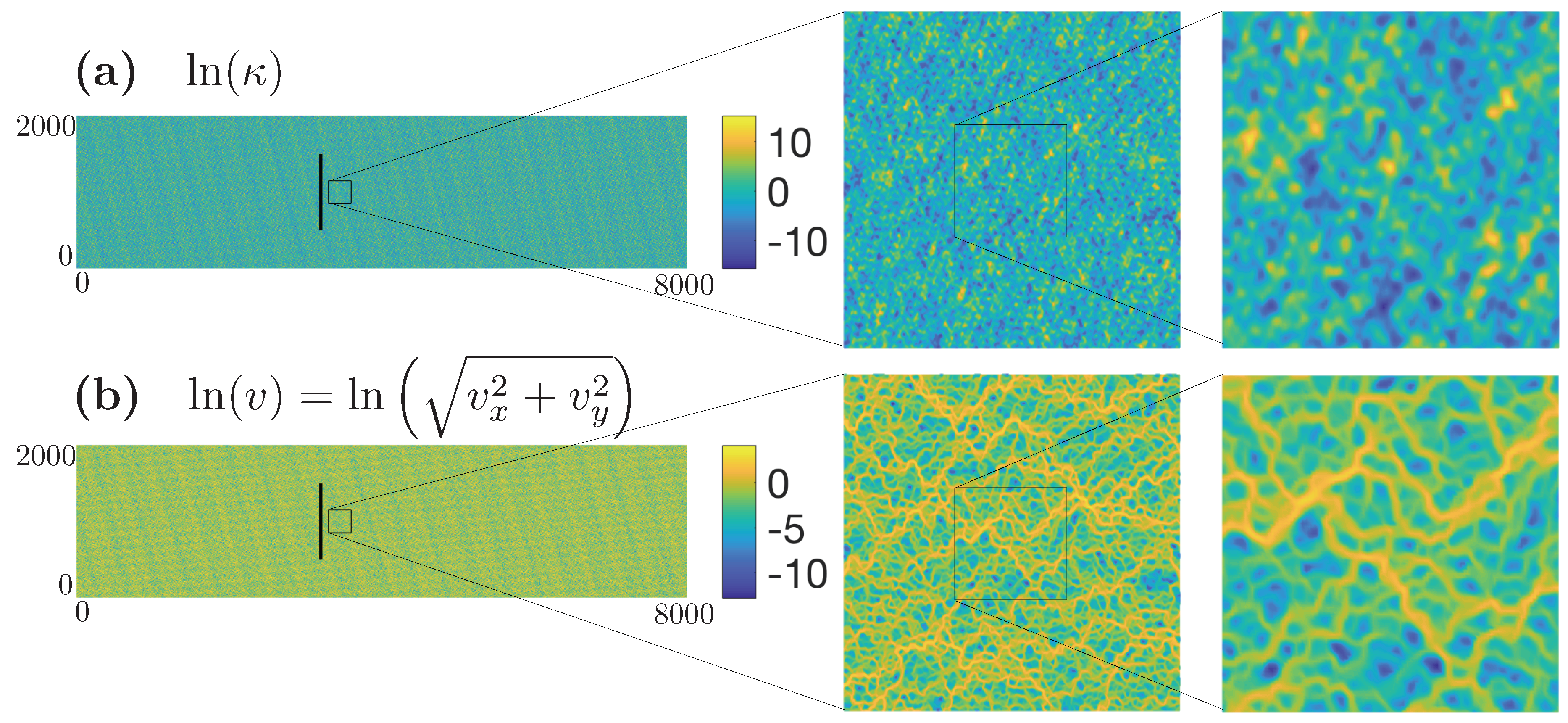
The velocity field considered in this work is representative of an idealized two-dimensional heterogeneous porous medium. To obtain the flow field, a log-normal random Gaussian-correlated permeability field (dimensions of ) is generated with zero mean and variance . The permeability is discretized in squared grid cells of unit length and we fix correlation length . The natural log of the permeability field used in this study is depicted in Figure 1a. The distribution, variance, and correlation length of the permeability field were chosen to align with the field used in the work of Le Borgne et al. [28,43], which first introduced the SMM and applied it to successfully predict mean transport characteristics, including the rate of spreading of the plume as quantified by the second centered moment as well as breakthrough curves. After generating our permeability field, we solve Darcy’s law coupled with incompressibility
to obtain our velocity fields, where v is the velocity , is pressure, and is viscosity. System (1) is solved using a finite volume method [57]. At the boundaries we impose permeameter like conditions: no flux across the lateral boundaries and constant head at the upstream and downstream boundaries. The mean velocity can then be rescaled to any desired value, so for convenience we choose . Figure 1b shows the natural log of the absolute value of the velocity , where and are the velocity fields in the horizontal and vertical directions, respectively. The flow domain was generated to be large enough so that when we simulate transport the solute will not interact with the boundaries. Domain lengths in the x and y directions equal to and , respectively, were deemed sufficient for this purpose.
The governing equation for transport is the advection dispersion equation
where C is the solute concentration and D is the constant isotropic dispersion coefficient . Our dispersion coefficient is selected to be a constant for simplicity and to align with the work of Le Borgne et al. [28,43], although it should be noted that using a velocity-dependent dispersion coefficient can have an impact on mixing [58,59]. Rather than solving Equation (2) directly, we model it with an equivalent particle tracking random walk approach. Our plume is discretized into a large number of particles. Each particle’s mass is given by , where is the total amount of mass of the solute, is the number of particles, and is the mass carried by each particle. , , and are chosen for this study. In this fully resolved model, the particles move in time according to Langevin equation
where , is the time step, and is the particle velocity interpolated from the velocity field shown in Figure 1b. At every time step, the particle moves with an advective step and a random jump reflecting diffusion with zero mean and a variance equal to .
We consider an advection-dominated flow with Péclet number equal to , where is the mean velocity in the horizontal direction of the flow, is the correlation length of the permeability field, and is the constant dispersion coefficient. Our simulation time step is . For our initial condition, we consider a flux-weighted line injection of a solute. The line injection is placed at between and , as indicated on Figure 1. This location was chosen so that the solute would not interact with the flow boundaries over the times that we are interested in measuring mixing.
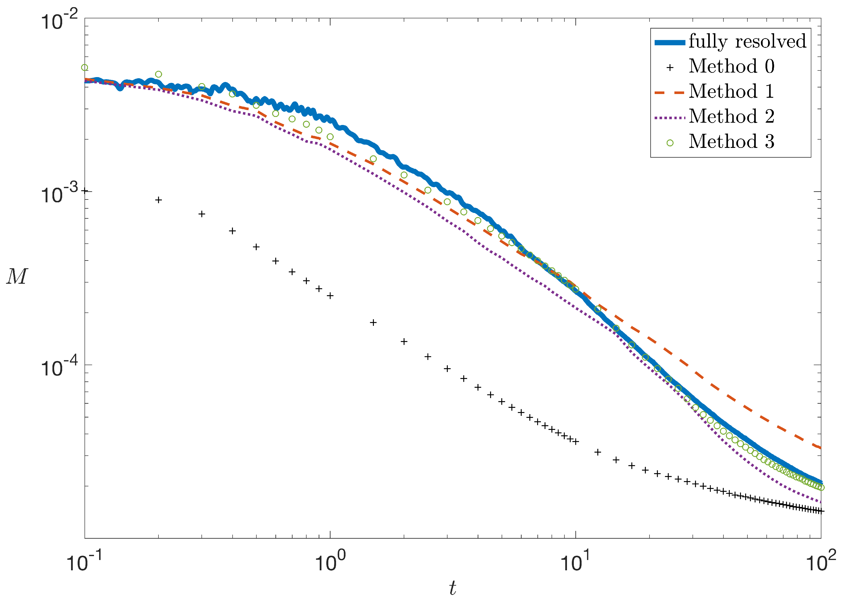
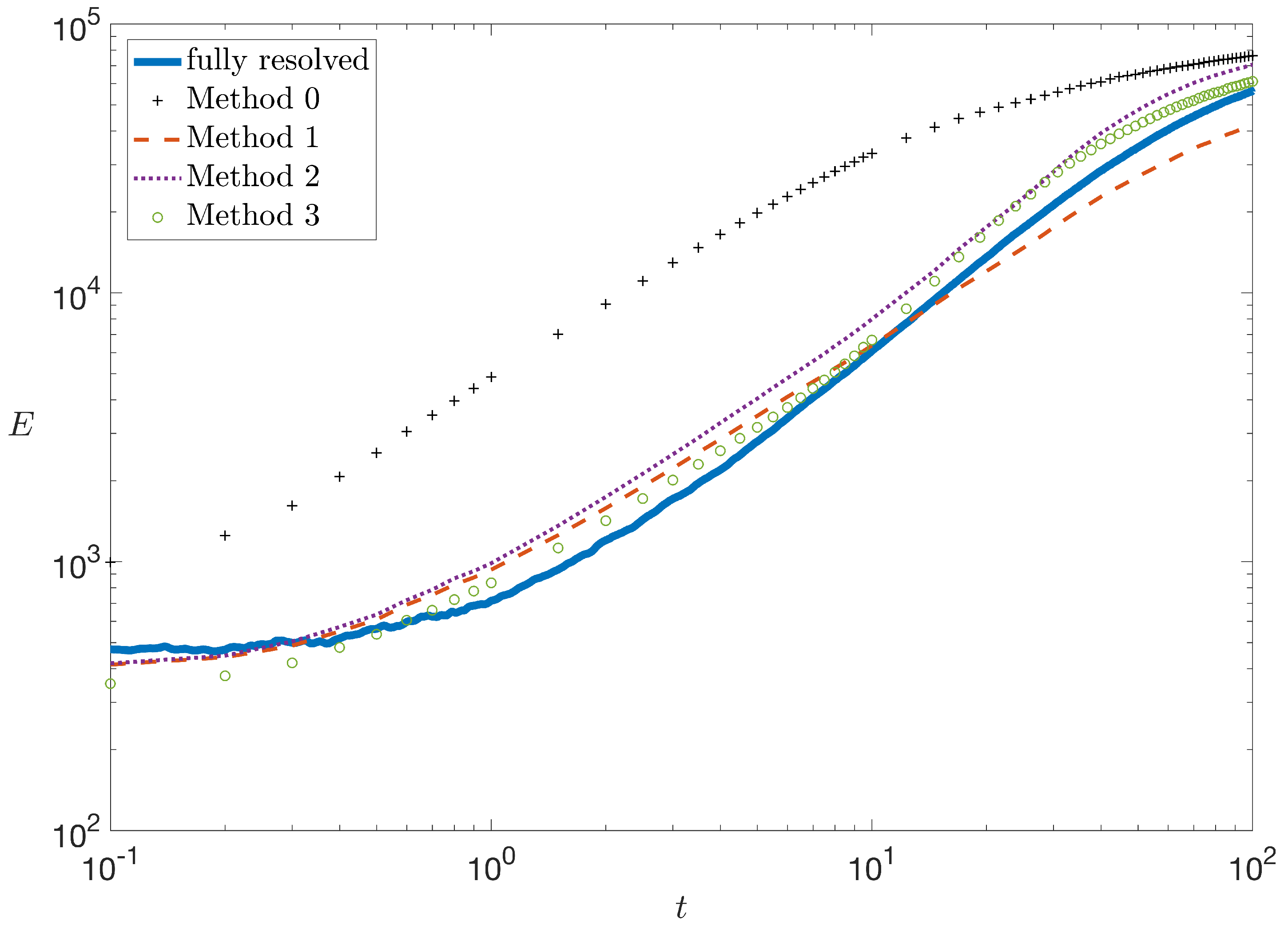
To quantify mixing in this system, we consider two commonly used metrics of global mixing. First, we measure the integral of the solute concentration squared, given by
describes how fluctuations in concentration evolve in time over the entire domain. The time derivative of this quantity multiplied by is known as the scalar dissipation rate and is a well-known metric used to quantify the rate of mixing [1,35,36]. Our second metric of mixing is the dilution index, defined as
The dilution index describes the degree of solute mass uniformity (i.e., dilution) in a system and is proportional to the volume occupied by a solute [37]. Under perfect mixing when is uniform over the entire domain under consideration, the integral of the squared concentration will be at a minimum, the scalar dissipation rate will be equal to zero, and the dilution index will be at a maximum.
In order to compute and , the concentration field must first be calculated. To obtain the concentration field, we map particles onto the same spatial grid as the velocity field. Then, the concentration in the ith grid cell is given by , where is the number of particles in the grid cell and is the area of the grid cell. Figure 2 and Figure 3 show the calculation of and in time from the fully resolved simulation using Equations (4) and (5), respectively (solid blue line). In the development of our upscaled model, our goal is to match the simulation results of this fully resolved simulation as well as possible.
3. Upscaled Model: Spatial Markov model
Next we describe the SMM and suite of modifications to the traditional method that were made for the purpose of predicting mixing. We provide a detailed overview of the SMM, but for more details refer the interested reader to the detailed descriptions provided in [54,60].
3.1. Model Parameterization
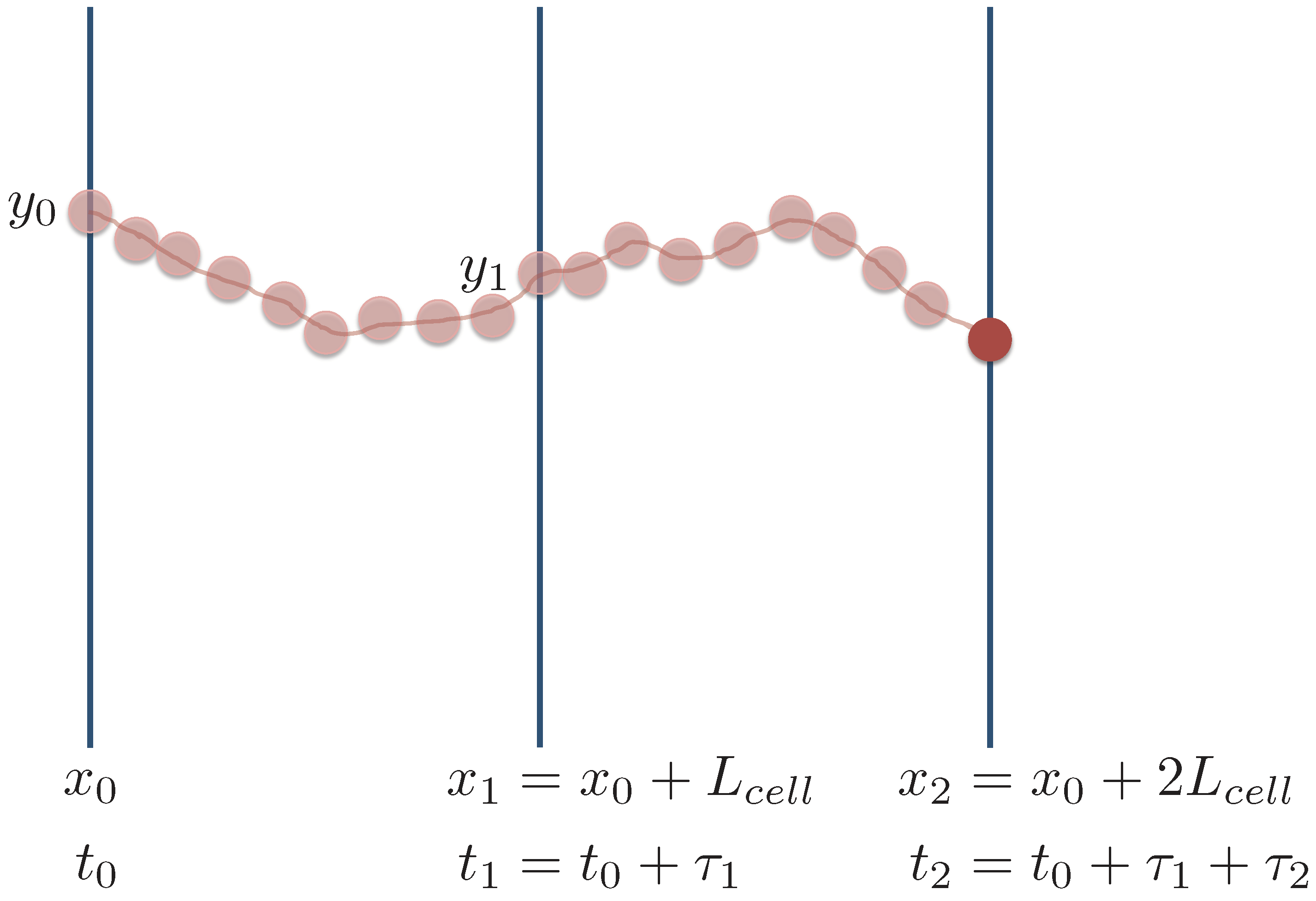
As in previous implementations of the SMM, we parameterize the model by running high resolution particle tracking simulations over two representative cells in our flow field using the random walk method described in the previous section using Equation (3). We initially have our flux weighted line injection located at and for our model parameterization we track the evolution of each of these particles in time until they have reached the downstream location . A cell length of was deemed appropriate for our system. Further discussion on this choice of cell length can be found in Section 3.2.1.
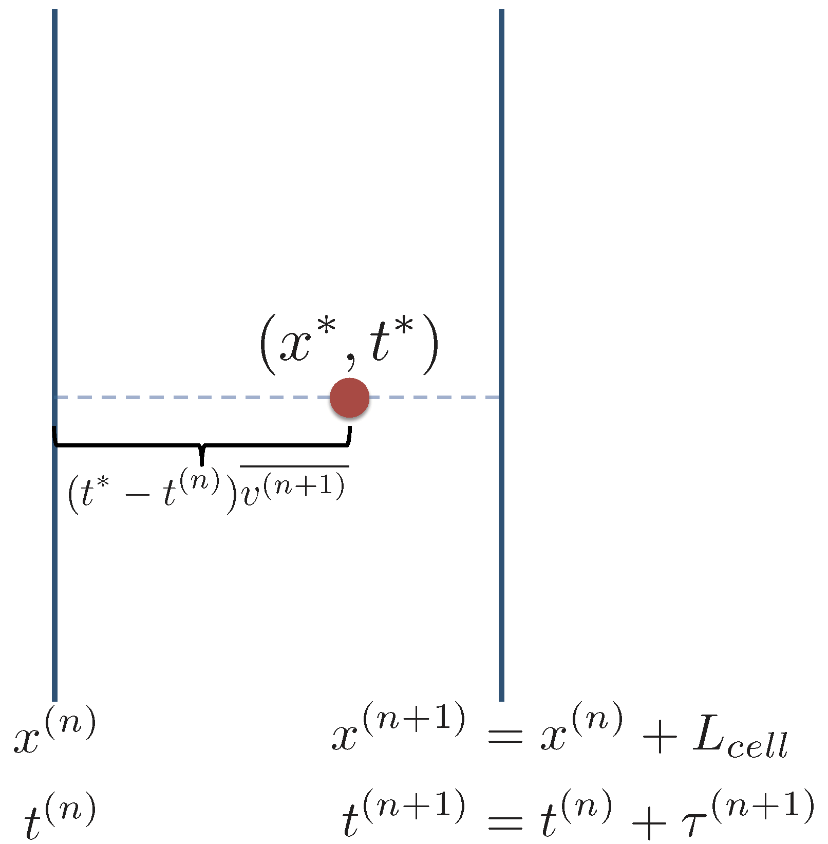
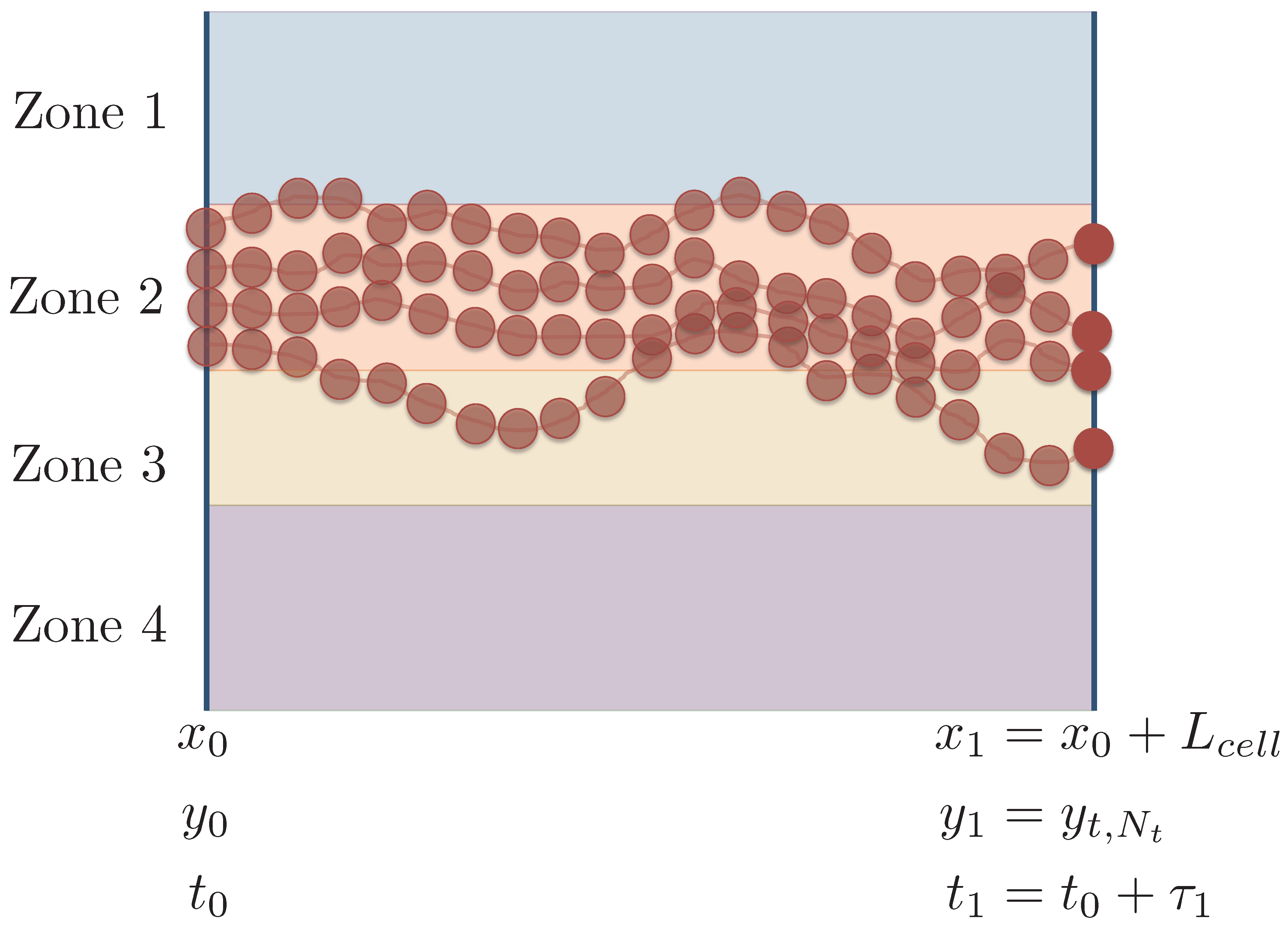
During the parameterization step, we record several features of a particle’s trajectory: (i) the particles’ y position at the inlet of the first cell (), (ii) the particles’ y position at the inlet of the second cell (), (iii) the time it takes for the particles to travel through the first cell (), and (iv) the time it takes for the particle to travel through the second cell (). This process is illustrated in Figure 4. After the joint distribution is obtained, it is used to inform the upscaled model. Typically, only and are recorded in the parameterization of the Spatial Markov model, but the additional information on and is required here for our downscaling procedure, which aims to predict mixing.
3.2. Model Mean Longitudinal Transport
The SMM is a random walk particle-based model. As for the fully resolved model described previously, the plume is discretized into a large number of particles of equal mass . Unlike the fully resolved model, a particle takes a uniform step in space of size and moves forward in time a random amount at each step in the upscaled model. In the SMM, during each model step, particles move forward in time and space according to Langevin equation
where is sampled from
The distribution of () is measured directly during the parameterization step and the distribution of given () is modeled by a transition matrix. To obtain the transition matrix, is separated into 20 equiprobable bins and the cutoff times associated with each bin are recorded. This bin number is chosen based on a convergence test and is in line with previous estimates for the required number of bins [60]. Bin 1 contains the particles with the fastest travel times and Bin 20 contains particles with the slowest travel times. A particle with travel time is in Bin i if , where is the cutoff time for Bin i, , and is greater than the maximum value of and for all particles. Then, the transition matrix is defined by
It is assumed that . Thus, each block of the transition matrix, , describes the probability that a particle will have a travel time in Bin j given that its travel time was in Bin i in the previous step.
Using Equation (6) in the SMM, we know when a particle is at a location , where N is an integer. In other words, at a specified time , the SMM provides information about which cell each particle is in, how long it has been there, and how long it will remain there, but the exact location of a given particle beyond this is unknown. In order to predict mixing by estimating or as defined in Equations (4) and (5), we need to have an estimate of the spatial distribution of the concentration field at a given moment in time. To obtain such information from the SMM, we must make an educated guess as to where a particle will be located within a cell. This means that we must develop a downscaling procedure within the upscaled model to predict the location of each particle. Note that we are not attempting to accurately reproduce the detailed concentration fields observed in the fully resolved model, but are instead trying to develop a downscaling procedure that provides an accurate estimate of the integral of the squared concentration, M, and the dilution index, E, in time—i.e., we are trying to generate a numerical closure via a downscaling process. In Section 4, we describe a variety of different downscaling methods considered here for the purpose of predicting mixing. While we actually implemented several more than those described here, we focus on this limited number to highlight specific features.
3.2.1. Choice of Cell Length
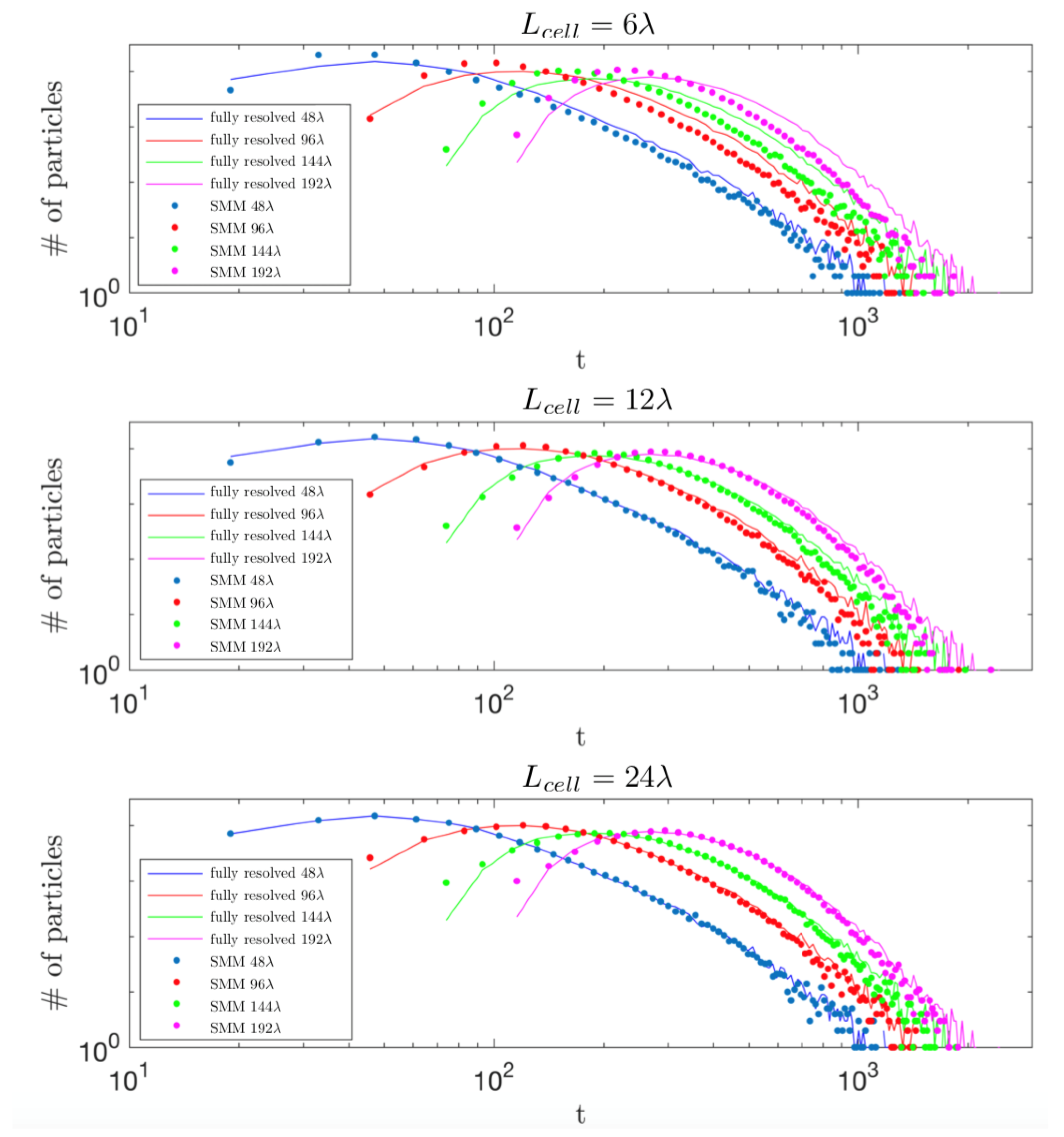
To determine the appropriate cell length, breakthrough curves (BTCs) were measured using the upscaled SMM at four downstream locations at distances 48λ, 96λ, 144λ, and 192λ from the inlet and compared to BTCs measured with the fully resolved model. The SMM was run using a variety of cell lengths in order to determine a cell length that would be appropriate for use in our expanded SMM to measure mixing. The BTCs measured using the SMM with cell lengths of = 6λ, 12λ, and 24λ (dotted lines) are shown on Figure 5 along with the corresponding BTCs measured with the fully resolved model (solid lines). The upscaled model should be able accurately capture the peaks and tails of the BTCs. By examination of Figure 5, it is clear that the upscaled model with is unable to capture either the peaks or the tails of the BTCs and the SMM results seem to deteriorate as the particles move downstream. For this reason, we must choose a larger cell length than for the SMM. From Figure 5, the SMM with appears to capture the peaks and tails of the BTCs relatively well, but gives better results. For this reason, a cell length of was deemed appropriate for our system. This result implies that a length scale of 24 is required to capture the transport dynamics in the heterogeneous system we consider. While limited to the specific level of heterogeneity investigated here, this result quantifies the characteristic scale necessary to identify the parameters of our effective transport model with respect to the one associated with the conductivity field. This scale is likely associated with connected structures (e.g., channels) emerging in the velocity field and that are relevant for the characterization of the travel time of successive jumps. This estimate is fully consistent with the detailed work of [61].
4. Downscaling Procedure to Predict Mixing
In this section we discuss the downscaling procedures developed in order to construct full concentration fields within the upscaled model. The goal here is not to accurately approximate the fully resolved concentration field, but rather reconstruct some effective concentration field that can be used to predict our desired global measures of mixing. To obtain this information, we must develop a procedure to estimate the x and y locations of each particle at any given time.
4.1. Downscaling the Streamwise Location x
As mentioned previously, at any time we know which cell each particle is in, how long it has been in that cell, and how much longer it will be there. Consider a particle that is in Cell at time . The particle will travel through that cell over an amount of time and has been in that cell for a time equal to , where is the total time traveled by the particle upon entering Cell . In order to make an educated guess for the x location of the particle within the cell at time , we assign each particle a mean longitudinal velocity through the cell equal to . For our downscaling procedure in x, we assume that the particle moves straight across Cell with a uniform velocity equal to . Thus, we linearly interpolate along this path to determine the downscaled x position, , i.e.,
This is the same choice for predicting x locations used in [53] and this process is illustrated schematically in Figure 6.
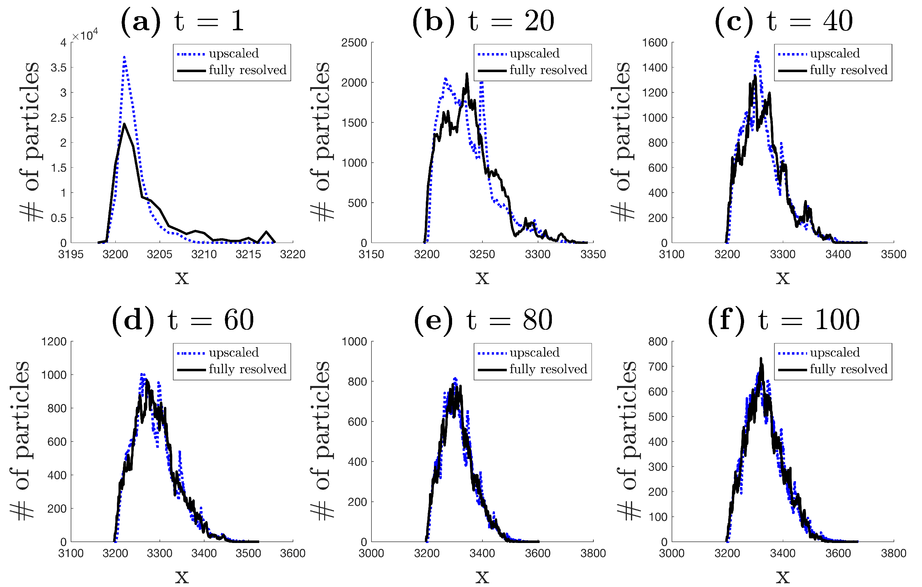
Figure 7 shows the histogram of particle x positions for both the fully resolved and upscaled models at various points in time throughout the simulation. This figure shows that the downscaling method described here does a reasonable job of predicting the x positions of particles relative to the small scale simulation. While it is certainly not perfect, we deem this sufficient and choose it as the method we will use to predict particle x locations for all cases. A feature that can be observed is that longitudinal particles’ locations are better matched as time advances (compare, for instance, results in Figure 7a–c to Figure 7d–f). This is consistent with the fact that our method considers a constant longitudinal velocity across a single step and therefore ignores subscale fluctuations that appear to average out across multiple steps of a single particle. Finding a good method to guess the y location of a given particles requires more effort, and we propose several different methods in the following sections.
4.2. Downscaling the Spanwise Location y
4.2.1. Method 0
Before developing more sophisticated downscaling procedures to predict the particle y locations, we start with probably the most naive approach; that is, we assume we know nothing about a particle’s y location and allow it to take any value with uniform probability between and . Thus, the downscaled x and y positions are given by
where . This method corresponds to a case where information about the probable y positions of particles is either unavailable or unimportant.
Figure 2 shows the calculation of M vs. time and Figure 3 shows E vs. time for both the fully resolved model and the upscaled model using Method 0. From Figure 2 and Figure 3, it is clear that Method 0 causes our upscaled model to strongly overpredict mixing. This result is unsurprising, as the placement of particles in the y direction based on a uniform distribution is equivalent to complete mixing of the solute in the y-direction. In reality, particles traveling on similar streamlines will tend to congregate with one another, leading to large transversal fluctuations in the concentration field. For this reason, a uniform distribution is not suitable here. More knowledge of the system is needed in order to adequately represent the particle y locations in the downscaling procedure.
4.2.2. Method 1
As observed in the previous section, it is crucial to incorporate more information from the system in the prediction of the particle positions in the y direction. Recall that in our parameterization step we recorded the joint distribution . For Method 1, we assign each particle in the upscaled model a y location equal to its initial y position, , at all times. Therefore, the downscaled x and y positions are given by
This process is illustrated in Figure 8. With this method, we are proposing that the particle’s initial position in y may be a sufficient approximation at all times in our upscaled model. From a statistical perspective this aligns with the idea that this might be its most likely location.
From Figure 2 and Figure 3, it is observed that there is a large improvement in the prediction of and using Method 1 relative to Method 0. This method does well at earlier times when particles have not moved very far from their initial position, but starts to under-predict mixing at ∼t = 10 as the particles have moved farther downstream and their initial y position is no longer as good of an approximation. This under-prediction of mixing can be attributed to the fact that particles would not move along a straight streamline in reality. This method does not allow for any form of transverse spreading, which is something that should be taken into account. Moving forward, we aim to improve this result by incorporating more information from the system.
4.2.3. Method 2
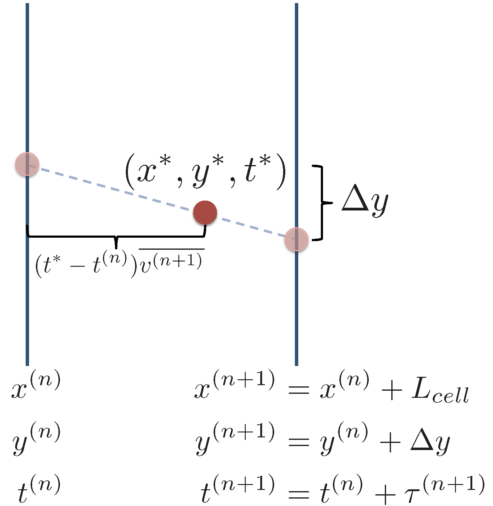
We know in reality that particles are not traveling along straight horizontal streamlines through our heterogeneous flow. The next step in improving our downscaling procedure would be to incorporate this idea and attempt to simulate a more realistic particle trajectory in our upscaled model. We adjust the Langevin equation to include a y component in our Spatial Markov model, i.e.,
Here, comes from , which was determined during the parameterization step of the model. Each value has an associated value; is drawn as usual using the transition matrix and its corresponding value is selected for each particle at every step. Then in the downscaling procedure, we linearly interpolate between and over the cell length to the point , i.e.,
This method is illustrated schematically in Figure 9.
The results of Method 2 in the calculation of and compared with the fully resolved model results are shown on Figure 2 and Figure 3, respectively. This method appears to show an improvement over Method 1, except at early times (before time = 10) when most of the particles are still in the first cell. It is worth noting that at all times throughout our simulation this method is over-predicting mixing. This can be attributed to the fact that Method 2 is not capable of incorporating the idea that particles traveling near each other are likely to have similar trajectories. In this version of the upscaled model, each particle draws a new (,) pair when it enters a new cell. The method is unable to account for the fact that particles traveling near each other will likely have similar and values. While values are correlated by the implementation of the transition matrix in the SMM, particles with similar travel times can have very different values of associated with them due to the highly heterogeneous nature of the flow field. This results in the observed over-mixing for Method 2 in Figure 2 and Figure 3.
4.2.4. Method 3
In this final method, we will add some complexity to the parameterization step of the model. We previously measured the joint distribution in the model parameterization. Now, we expand this step by recording information on the particle trajectories within the first cell. To measure these trajectories, we record the y positions for each particle as they travel across the first cell at evenly spaced points in the x-direction. Therefore, in our updated parameterization step we record the joint distribution , where are the particle y positions measured at points along their trajectory. was determined to be a sufficient number of sampling positions for capturing the particle trajectories within the cell.
In order to incorporate this additional particle trajectory information into our downscaling procedure, we separate the particles into zones based on their initial y position, . These zones were defined by separating the particle positions into a number of equiprobable regions. Since our solute line injection defined by the particle positions is flux-weighted, these equiprobable zones will not be uniformly spaced in the y direction. was selected here, so that each zone will contain trajectory information from particles. A broad range of zone numbers were tested and the results were not significantly affected, indicating the robustness of this method. The histogram of values is shown in Figure 10a, where each color represents a different zone number.
After defining our zones, we then create a set of y values, , for each zone number j. The set contains all of the y positions measured in the trajectories for every particle that had in Zone j. This means that contains every y value from each particle trajectory defined by that had its initial y position, , located in zone number j. In this study, is a set containing y values. Figure 10b shows the histogram of the set of y values for each zone number j. The adjustment of the parameterization step is illustrated in Figure 11.
After defining our zones and determining the set of y values associated with each zone number j, we will now use this information in our downscaling procedure. In this method, we will determine the downscaled y position of each particle at some time by randomly selecting a y value from the set of possible y values, , associated with each particle’s zone number j. The particle’s zone number depends exclusively on its initial y position, , and does not change at any point throughout the simulation. For example, a particle that had in Zone 2 will always draw from the set of possible y values associated with that zone, . Thus, the downscaled x and y positions at time are given by
where is a y value selected randomly with uniform probability at each Spatial Markov step from the set associated with the particle’s zone number j.
This method incorporates the idea that particles will in general travel along paths that have y values similar to their initial y position. They will not likely be making large jumps in the y direction, but they will also not simply maintain their initial y position as we assumed in Method 1. By selecting from a set of y values based on each particle’s initial y position, we are assuming that particles over time will have the same distribution in y as they did in the first cell during the model parameterization. The y positions of particles are assigned through a regionalization of the transversal dimension y into zones, preventing them from making excessively large jumps in the spanwise direction. The results of Method 3 in the measurement of and compared to the fully resolved model and the other upscaled models are shown on Figure 2 and Figure 3, respectively. As observed in these figures, Method 3 performs better than the other upscaled models in estimating and .
5. Discussion
Now, we compare the different upscaled methods both qualitatively and quantitatively. From Figure 2 and Figure 3, it is clear that Methods 1, 2, and 3 all perform very well relative to Method 0 in predicting and as compared to the fully resolved random walk algorithm. Here, we will discuss the successes of each of these methods as well as their shortcomings.
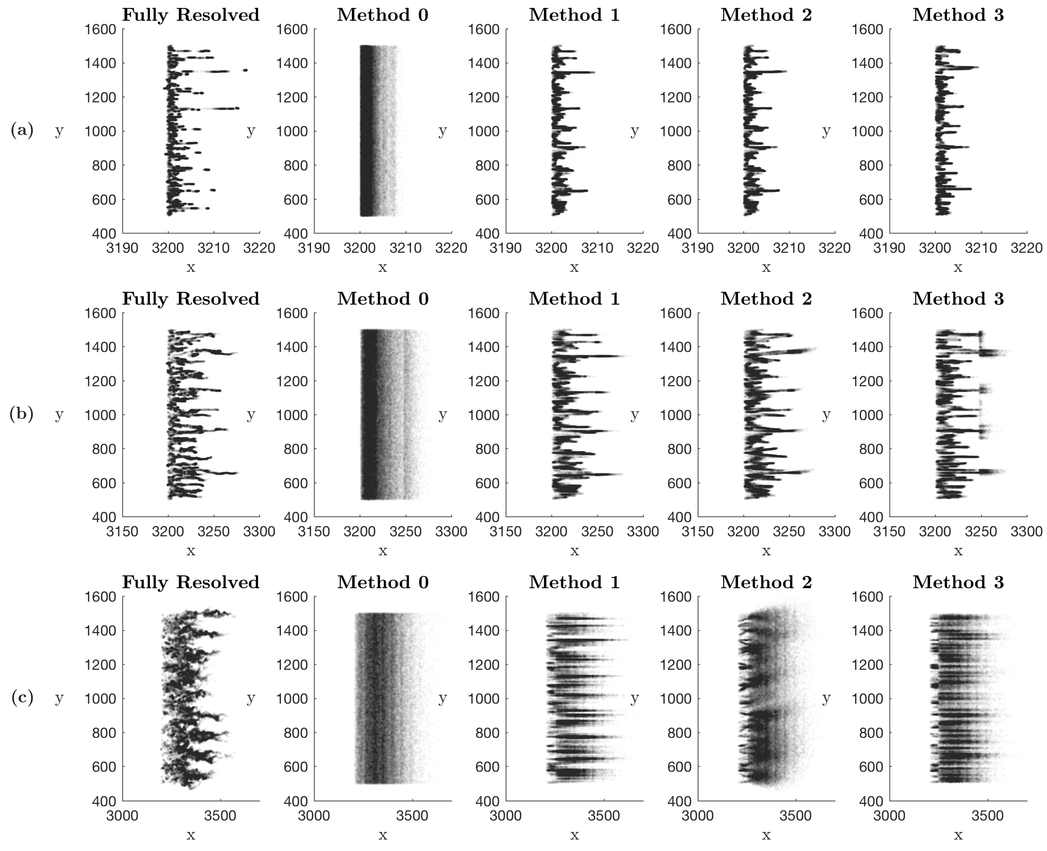
Figure 12 shows the particle locations at three different times throughout the simulations for the fully resolved random walk model and the upscaled methods 0, 1, 2, and 3. As already noted above, our goal was not necessarily to reproduce the concentration fields of the fully resolved simulation, but to capture the key features that enable an accurate estimate of and , such as the peaks in concentration and the spreading of the plume. Many closures for predicting reactive transport involve integrated nonlinear terms like these e.g., [62,63] and so accurately estimating them is an essential first step to accurate upscaling of reactive transport. As observed in Figure 12, Method 0 clearly over-predicts mixing at all times. This is consistent with the results of Figure 2 and Figure 3. In Figure 12, Method 1 qualitatively appears similar to our fully resolved simulations at and 10, but it appears that the concentration peaks may be too high and there is not enough spreading of the plume at . This is in agreement with the under-prediction of mixing observed for Method 1 after in Figure 2 and Figure 3. Methods 2 and 3 also appear qualitatively similar to the fully resolved simulation at and 10, but may have slightly too much spreading. It is also observed in Figure 12 that there is some discontinuous structure for Method 3 at . This corresponds to the point in time where the particles have begun to enter the second SMM cell. At each step in the SMM, each particle selects a new y value from the set associated with that particle’s zone number j. This means that as a particle enters a new SMM cell it selects a new y value that is somewhere between the minimum and maximum values of , resulting in the observed structure. At , Method 2 clearly has too much spreading, but may still be capturing the peaks in concentration. Figure 2 and Figure 3 are in agreement with these observations as Method 2 slightly over-predicts mixing at all times after . At , the plume of Method 3 has a different shape than the fully resolved simulation, but the amount of spreading and regions of high concentration are comparable. Figure 2 and Figure 3 show that Method 3 also very slightly over-predicts mixing at all times except very early times, but in general show results that are very close to that of the fully resolved simulation. Upon visual inspection of Figure 2 and Figure 3, Method 3 appears to give the best prediction of and .
After qualitatively examining each of these methods, we now want to quantify which method performs the best. To do this, we use the mean absolute error on a log scale, defined as
where is either or , is the mixing metric calculated in the fully resolved model, is the mixing metric calculated in the upscaled model, and is the number of points in time at which and are measured. We choose to calculate the mean absolute error on a log scale so as not to penalize the smaller values of and . The results of this error calculation are shown in Table 1. As expected, Method 0 has a significantly larger error than Methods 1, 2, and 3. Methods 1 and 2 had very similar error values, and Method 3 had the smallest error in the measurement of both and . Based on this error metric, Method 3 is the option that performs the best. This is consistent with the qualitative examination as well.
6. Conclusions
In this work, we have extended the Spatial Markov model to predict effective mixing in flows through idealized two-dimensional heterogeneous porous media. To do this, we developed several downscaling methods to predict the particle locations within the upscaled model and thereby approximating solute distribution within the domain. From these predicted particle locations, we were able to generate concentration fields that could then be used to calculate the evolution of the solute mixing, as quantified by integral of the squared concentration, , and the dilution index, , in time. The results of each of these downscaling methods developed for the SMM were compared to a fully resolved random walk simulation. In order to be able to predict and accurately with our upscaled model, it was crucial to capture the same amount of variation in the concentration field as in the fully resolved model. Each of these upscaled methods require nearly the same computation time and are on the order of 1000 times faster to run than the fully resolved method. Although Method 3 does add more complexity to the upscaled model than the other methods presented here, it is as computationally efficient as the other methods and provides the best prediction of and . For this reason, we recommend Method 3 as an extension of the Spatial Markov model to predict mixing in uniform mean flow simulations in heterogeneous porous media.
Although we were able to predict and within an acceptable margin of error using our upscaled model, there is still room for improvement. Our results show that a key feature to be encoded in the upscaled approaches is that particles traveling near each other will have similar trajectories. Method 3 provides good results in terms of matching average mixing behavior through a rough regionalization of transversal particle positions. Still, we observe a slight over-prediction of mixing and the methodology is not able to capture the topological structure of the solute plume. We envision that the method can be further improved in future works, particularly with the aim of generalizing the approach to broader transport settings beyond one-dimensional transport.
Author Contributions
Conceptualization, E.E.W., G.M.P. and D.B.; methodology, E.E.W., N.L.S., G.M.P., D.H.R. and D.B.; software, E.E.W.; validation, E.E.W. and N.L.S.; formal analysis, E.E.W., N.L.S., G.M.P., D.H.R. and D.B.; investigation, E.E.W.; resources, E.E.W., N.L.S., G.M.P., D.H.R., D.B.; data curation, E.E.W.; writing—original draft preparation, E.E.W.; writing—review and editing, E.E.W., N.L.S., G.M.P., D.H.R., D.B.; visualization, E.E.W.; supervision, N.L.S., G.M.P., D.H.R., D.B.; project administration, E.E.W., D.H.R., D.B.; funding acquisition, D.B.
Funding
This material is based upon work supported by, or in part by, the US Army Research Office under Contract/Grant number W911NF-18-1-0338. The authors were also supported by the National Science Foundation under awards EAR-1351623 and EAR-1446236.
Conflicts of Interest
The authors declare no conflict of interest.
References
- Engdahl, N.B. Scalar dissipation rates in non-conservative transport systems. J. Contam. Hydrol. 2013, 46–60. [Google Scholar] [CrossRef]
- Dentz, M.; Le Borgne, T.; Englert, A.; Bijeljic, B. Mixing, spreading and reaction in heterogeneous media: A brief review. J. Contam. Hydrol. 2011, 120–121, 1–17. [Google Scholar] [CrossRef] [PubMed]
- Le Borgne, T.; Ginn, T.R.; Dentz, M. Impact of fluid deformation on mixing-induced chemical reactions in heterogeneous flows. Geophys. Res. Lett. 2014, 41, 7898–7906. [Google Scholar] [CrossRef] [Green Version]
- Valocchi, A.J.; Bolster, D.; Werth, C.J. Mixing-Limited Reactions in Porous Media. Transp. Porous Media 2018. [Google Scholar] [CrossRef]
- Kang, K.; Redner, S. Scaling approach for the kinetics of recombination processes. Phys. Rev. Lett. 1984, 52, 955–958. [Google Scholar] [CrossRef]
- Ovchinnikov, A.A.; Zeldovich, Y.B. Role of density fluctuations in bimolecular reaction kinetics. Chem. Phys. 1978, 28, 215–218. [Google Scholar] [CrossRef]
- Toussaint, D.; Wilczec, F. Particle–antiparticle annihilation in diffusive motion. J. Chem. Phys. 1983, 78, 2642. [Google Scholar] [CrossRef]
- Bolster, D.; Benson, D.A.; Le Borgne, T.; Dentz, M. Anomalous mixing and reaction induced by superdiffusive nonlocal transport. Phys. Rev. E 2010, 82, 021119. [Google Scholar] [CrossRef]
- Ding, D.; Benson, D.A.; Paster, A.; Bolster, D. Modeling bimolecular reactions and transport in porous media via particle tracking. Adv. Water Resour. 2013, 53, 56–65. [Google Scholar] [CrossRef] [Green Version]
- Bolster, D.; de Anna, P.; Benson, D.A.; Tartakovsky, A.M. Incomplete mixing and reactions with fractional dispersion. Adv. Water Resour. 2012, 37, 86–93. [Google Scholar] [CrossRef]
- Gramling, C.; Harvey, C.; Meigs, L. Reactive Transport in Porous Media: A Comparison of Model Prediction with Laboratory Visualization. Environ. Sci. Technol. 2002, 36, 2508–2514. [Google Scholar] [CrossRef] [PubMed]
- Monson, E.; Kopelman, R. Observation of laser speckle effects and nonclassical kinetics in an elementary chemical reaction. Phys. Rev. Lett. 2000, 85, 666–669. [Google Scholar] [CrossRef] [PubMed]
- Monson, E.; Kopelman, R. Nonclassical kinetics of an elementary A+B->C reaction-diffusion system showing effects of a speckled initial reactant distribution and eventual self-segregation: Experiments. Phys. Rev. E Stat. Nonlinear Soft Matter Phys. 2004, 69, 1–12. [Google Scholar] [CrossRef]
- Raje, D.S.; Kapoor, V. Experimental study of bimolecular reaction kinetics in porous media. Environ. Sci. Technol. 2000, 34, 1234–1239. [Google Scholar] [CrossRef]
- Castro-Alcalá, E.; Fernàndez-Garcia, D.; Carrera, J.; Bolster, D. Visualization of mixing processes in a heterogeneous sand box aquifer. Environ. Sci. Technol. 2012, 46, 3228–3235. [Google Scholar] [CrossRef] [PubMed]
- Ding, D.; Benson, D.A.; Fernàndez-Garcia, D.; Henri, C.V.; Hyndman, D.W.; Phanikumar, M.S.; Bolster, D. Elimination of the Reaction Rate “Scale Effect”: Application of the Lagrangian Reactive Particle-Tracking Method to Simulate Mixing-Limited, Field-Scale Biodegradation at the Schoolcraft (MI, USA) Site. Water Resour. Res. 2017, 53, 10411–10432. [Google Scholar] [CrossRef] [Green Version]
- Guerra, P.; Gonzalez, C.; Escauriaza, C.; Pizarro, G.; Pasten, P. Incomplete Mixing in the Fate and Transport of Arsenic at a River Affected by Acid Drainage. Water Air Soil Pollut. 2016, 227. [Google Scholar] [CrossRef]
- Kang, P.K.; Bresciani, E.; An, S.; Lee, S. Impact of pore-scale incomplete mixing on biodegradation in aquifers: From batch experiment to field-scale modeling. Adv. Water Resour. 2019, 123, 1–39. [Google Scholar] [CrossRef]
- Kapoor, V.; Jafvert, C.T.; Lyn, D.A. Experimental study of a bimolecular reaction in Poiseuille flow. Water Resour. Res. 1998, 34, 1997–2004. [Google Scholar] [CrossRef]
- Chiogna, G.; Bellin, A. Analytical solution for reactive solute transport considering incomplete mixing within a reference elementary volume. Water Resour. Res. 2013, 49, 2589–2600. [Google Scholar] [CrossRef] [Green Version]
- Ginn, T.R. Modeling Bimolecular Reactive Transport With Mixing-Limitation: Theory and Application to Column Experiments. Water Resour. Res. 2018, 54, 256–270. [Google Scholar] [CrossRef]
- Benson, D.A.; Pankavich, S.; Bolster, D. On the separate treatment of mixing and spreading by the reactive-particle-tracking algorithm: An example of accurate upscaling of reactive Poiseuille flow. Adv. Water Resour. 2019, 123, 40–53. [Google Scholar] [CrossRef]
- Steefel, C.I.; DePaolo, D.J.; Lichtner, P.C. Reactive transport modeling: An essential tool and a new research approach for the Earth sciences. Earth Planet. Sci. Lett. 2005, 240, 539–558. [Google Scholar] [CrossRef]
- Yeh, G.T.; Tripathi, V.S. A Critical Evaluation of Recent Developments in Hydrogeochemical Transport Models of Reactive Multichemical Components. Water Resour. Res. 1989, 25, 93–108. [Google Scholar] [CrossRef]
- Mayer, K.U.; Benner, S.G.; Blowes, D.W. Process-based reactive transport modeling of a permeable reactive barrier for the treatment of mine drainage. J. Contam. Hydrol. 2006, 85, 195–211. [Google Scholar] [CrossRef]
- Knutson, C.; Valocchi, A.; Werth, C. Comparison of continuum and pore-scale models of nutrient biodegradation under transverse mixing conditions. Adv. Water Resour. 2007, 30, 1421–1431. [Google Scholar] [CrossRef]
- Le Borgne, T.; De Dreuzy, J.R.; Davy, P.; Bour, O. Characterization of the velocity field organization in heterogeneous media by conditional correlation. Water Resour. Res. 2007, 43, 1–10. [Google Scholar] [CrossRef]
- Le Borgne, T.; Dentz, M.; Carrera, J. Lagrangian statistical model for transport in highly heterogeneous velocity fields. Phys. Rev. Lett. 2008, 101, 1–4. [Google Scholar] [CrossRef]
- Weeks, S.W.; Sposito, G. Mixing and stretching efficiency in steady and unsteady groundwater flows. Water Resour. Res. 1998, 34, 3315–3322. [Google Scholar] [CrossRef] [Green Version]
- De Barros, F.P.J.; Dentz, M.; Koch, J.; Nowak, W. Flow topology and scalar mixing in spatially heterogeneous flow fields. Geophys. Res. Lett. 2012, 39, 1–5. [Google Scholar] [CrossRef]
- Le Borgne, T.; Dentz, M.; Villermaux, E. Stretching, coalescence, and mixing in porous media. Phys. Rev. Lett. 2013, 110, 204501. [Google Scholar] [CrossRef] [PubMed]
- Edery, Y.; Porta, G.M.; Guadagnini, A.; Scher, H.; Berkowitz, B. Characterization of Bimolecular Reactive Transport in Heterogeneous Porous Media. Transp. Porous Media 2016, 115, 291–310. [Google Scholar] [CrossRef]
- Trefry, M.; Lester, D.; Metcalfe, G.; Wu, J. Natural Groundwater Systems Can Display Chaotic Mixing at the Darcy Scale. arXiv, 2018; arXiv:1808.03641. [Google Scholar]
- Ye, Y.; Chiogna, G.; Lu, C.; Rolle, M. Effect of Anisotropy Structure on Plume Entropy and Reactive Mixing in Helical Flows. Transp. Porous Media 2018, 121, 315–332. [Google Scholar] [CrossRef]
- Bolster, D.; Dentz, M.; Le Borgne, T. Hypermixing in linear shear flow. Water Resour. Res. 2011, 47, 1–4. [Google Scholar] [CrossRef]
- Le Borgne, T.; Dentz, M.; Bolster, D.; Carrera, J.; de Dreuzy, J.R.; Davy, P. Non-Fickian mixing: Temporal evolution of the scalar dissipation rate in heterogeneous porous media. Adv. Water Resour. 2010, 33, 1468–1475. [Google Scholar] [CrossRef]
- Kitanidis, P.K. The concept of the Dilution Index. Water Resour. Res. 1994, 30, 2011–2026. [Google Scholar] [CrossRef]
- Engdahl, N.B.; Benson, D.A.; Bolster, D. Predicting the enhancement of mixing-driven reactions in nonuniform flows using measures of flow topology. Phys. Rev. E 2014, 90, 1–5. [Google Scholar] [CrossRef] [PubMed]
- Aquino, T.; Bolster, D. Localized Point Mixing Rate Potential in Heterogeneous Velocity Fields. Transp. Porous Media 2017, 119, 391–402. [Google Scholar] [CrossRef]
- Wright, E.E.; Richter, D.H.; Bolster, D. Effects of incomplete mixing on reactive transport in flows through heterogeneous porous media. Phys. Rev. Fluids 2017, 2, 114501. [Google Scholar] [CrossRef]
- De Dreuzy, J.R.; Carrera, J. On the validity of effective formulations for transport through heterogeneous porous media. Hydrol. Earth Syst. Sci. 2016, 20, 1319–1330. [Google Scholar] [CrossRef] [Green Version]
- Edery, Y.; Guadagnini, A.; Scher, H.; Berkowitz, B. Origins of anomalous transport in heterogeneous media: Structural and dynamic controls. Water Resour. Res. 2014, 50, 1490–1505. [Google Scholar] [CrossRef] [Green Version]
- Le Borgne, T.; Dentz, M.; Carrera, J. Spatial Markov processes for modeling Lagrangian particle dynamics in heterogeneous porous media. Phys. Rev. E Stat. Nonlinear Soft Matter Phys. 2008, 78, 1–9. [Google Scholar] [CrossRef] [PubMed]
- Kang, P.K.; Dentz, M.; Le Borgne, T.; Juanes, R. Spatial Markov model of anomalous transport through random lattice networks. Phys. Rev. Lett. 2011, 107, 1–5. [Google Scholar] [CrossRef] [PubMed]
- Kang, P.K.; Borgne, T.L.; Dentz, M.; Bour, O.; Juanes, R.; Kang, P.; Borgne, T.L.; Dentz, M.; Bour, O.; Juanes, R. Impact of velocity correlation and distribution on transport in fractured media: Field evidence and theoretical model. Water Resour. Res. 2015, 940–959. [Google Scholar] [CrossRef]
- Kang, P.K.; Dentz, M.; Le Borgne, T.; Lee, S.; Juanes, R. Anomalous transport in disordered fracture networks: Spatial Markov model for dispersion with variable injection modes. Adv. Water Resour. 2017, 106, 80–94. [Google Scholar] [CrossRef] [Green Version]
- Kang, P.K.; Dentz, M.; Juanes, R. Predictability of anomalous transport on lattice networks with quenched disorder. Phys. Rev. E 2011, 83, 030101. [Google Scholar] [CrossRef] [PubMed]
- Kang, P.K.; Anna, P.; Nunes, J.P.; Bijeljic, B.; Blunt, M.J.; Juanes, R. Pore-scale intermittent velocity structure underpinning anomalous transport through 3-D porous media. Geophys. Res. Lett. 2014, 41, 6184–6190. [Google Scholar] [CrossRef] [Green Version]
- Kang, P.K.; Dentz, M.; Le Borgne, T.; Juanes, R. Anomalous transport on regular fracture networks: Impact of conductivity heterogeneity and mixing at fracture intersections. Phys. Rev. E 2015, 92, 022148. [Google Scholar] [CrossRef] [PubMed]
- Kang, P.K.; Brown, S.; Juanes, R. Emergence of anomalous transport in stressed rough fractures. Earth Planet. Sci. Lett. 2016, 454, 46–54. [Google Scholar] [CrossRef] [Green Version]
- De Anna, P.; Le Borgne, T.; Dentz, M.; Tartakovsky, A.M.; Bolster, D.; Davy, P. Flow intermittency, dispersion, and correlated continuous time random walks in porous media. Phys. Rev. Lett. 2013, 110, 184502. [Google Scholar] [CrossRef]
- Sund, N.L.; Bolster, D.; Dawson, C. Upscaling transport of a reacting solute through a peridocially converging-diverging channel at pre-asymptotic times. J. Contam. Hydrol. 2015, 182, 1–15. [Google Scholar] [CrossRef] [PubMed]
- Sund, N.; Porta, G.; Bolster, D.; Parashar, R. A Lagrangian transport Eulerian reaction spatial (LATERS) Markov model for prediction of effective bimolecular reactive transport. Water Resour. Res. 2017, 53, 9040–9058. [Google Scholar] [CrossRef]
- Bolster, D.; Méheust, Y.; Le Borgne, T.; Bouquain, J.; Davy, P. Modeling preasymptotic transport in flows with significant inertial and trapping effects—The importance of velocity correlations and a spatial Markov model. Adv. Water Resour. 2014, 70, 89–103. [Google Scholar] [CrossRef]
- Sund, N.; Bolster, D.; Mattis, S.; Dawson, C. Pre-asymptotic Transport Upscaling in Inertial and Unsteady Flows through Porous Media. Transp. Porous Media 2015, 109, 411–432. [Google Scholar] [CrossRef]
- Sund, N.L.; Porta, G.M.; Bolster, D. Upscaling of dilution and mixing using a trajectory based Spatial Markov random walk model in a periodic flow domain. Adv. Water Resour. 2017, 103, 76–85. [Google Scholar] [CrossRef]
- Aarnes, J.E.; Gimse, T.; Lie, K.A. An introduction to the numerics of flow in porous media using Matlab. In Geometric Modelling, Numerical Simulation, and Optimization; Springer: Berlin/Heidelberg, Germany, 2007; pp. 265–306. [Google Scholar]
- Wen, B.; Chang, K.W.; Laboratories, S.N.; Hesse, M.A. Rayleigh-Darcy convection with hydrodynamic dispersion. Phys. Rev. Fluids 2018, 123801, 1–18. [Google Scholar] [CrossRef]
- Wang, L.; Nakanishi, Y.; Hyodo, A.; Suekane, T. Three-dimensional structure of natural convection in a porous medium: Effect of dispersion on finger structure. Int. J. Greenh. Gas Control 2016, 53, 274–283. [Google Scholar] [CrossRef]
- Le Borgne, T.; Bolster, D.; Dentz, M.; De Anna, P.; Tartakovsky, A. Effective pore-scale dispersion upscaling with a correlated continuous time random walk approach. Water Resour. Res. 2011, 47, 1–10. [Google Scholar] [CrossRef]
- Hakoun, V.; Comolli, A.; Dentz, M. From medium heterogeneity to flow and transport: A time-domain random walk approach. In Proceedings of the AGU Fall Meeting, New Orleans, OR, USA, 11–15 December 2017. [Google Scholar]
- Porta, G.M.; Riva, M.; Guadagnini, A. Upscaling solute transport in porous media in the presence of an irreversible bimolecular reaction. Adv. Water Resour. 2012, 35, 151–162. [Google Scholar] [CrossRef]
- Tartakovsky, A.M.; de Anna, P.; Le Borgne, T.; Balter, A.; Bolster, D. Effect of spatial concentration fluctuations on effective kinetics in diffusion-reaction systems. Water Resour. Res. 2012, 48, W02526. [Google Scholar] [CrossRef]
Figure 1.
(a) The natural log of the permeability field and (b) the natural log of the absolute value of the velocity v = , where and are the velocity fields in the horizontal and vertical flow directions, respectively. The solid black line on each of the fields indicates the location of the solute line injection and the small squares indicate regions which we have zoomed in on so the flow features could be seen more clearly on the right side of the figure.

Figure 2.
The integral of the squared concentration, M, versus time for the fully resolved random walk model and the different versions of the upscaled model described in Section 4.
Figure 2.
The integral of the squared concentration, M, versus time for the fully resolved random walk model and the different versions of the upscaled model described in Section 4.

Figure 3.
The dilution index, E, versus time for the fully resolved random walk model and the different versions of the upscaled model described in Section 4.
Figure 3.
The dilution index, E, versus time for the fully resolved random walk model and the different versions of the upscaled model described in Section 4.

Figure 4.
Diagram illustrating the parameterization step for the upscaled model. Each particle moves by random walk over a distance of two cell lengths and the particle’s initial y position (), y position at the inlet of the second cell (), and travel times through the first and second cells ( and , respectively) are recorded. The red circles represent an example of a single particle trajectory.

Figure 5.
Breakthrough curves measured at distances 48, 96, 144, and 192 downstream from the inlet for both the fully resolved model (solid lines) and the Spatial Markov model (dotted lines) with cell lengths of (top) 6λ, (middle) 12λ, and (bottom) 24λ. From these results, it was determined that a cell length of 24λ was an appropriate choice for our upscaled model.

Figure 6.
Illustration of the downscaling procedure in the x direction. A particle is in Cell and will travel through that cell over an amount of time . We want to determine the particle’s x location at time .
Figure 6.
Illustration of the downscaling procedure in the x direction. A particle is in Cell and will travel through that cell over an amount of time . We want to determine the particle’s x location at time .

Figure 7.
Histogram of particle x locations at times (a) t = 1, (b) t = 20, (c) t = 40, (d) t = 60, (e) t = 80, and (f) t = 100 for both the fully resolved particle tracking simulations (solid black line) and the Spatial Markov model with the downscaling method described in Section 4.1 (dashed blue line). The bin size selected for the histogram is the same as the fully resolved grid resolution.

Figure 8.
Illustration of the downscaling procedure Method 1 in the y direction. A particle is in Cell and will travel through that cell over an amount of time . The particle’s x location is determined using the method described in Section 4.1. We want to predict the particle’s y location at time . In this method, the downscaled y location is equal to each particle’s initial y position, .

Figure 9.
Illustration of the downscaling procedure Method 2 in the y direction. A particle is in Cell and will travel through that cell over an amount of time . The particle’s x location is determined using the method described in Section 4.1. We predict the particle’s y location at time using Method 2.

Figure 10.
(a) The distribution of separated into equiprobable zones and (b) the distribution of y values for each zone calculated in the parameterization step.
Figure 10.
(a) The distribution of separated into equiprobable zones and (b) the distribution of y values for each zone calculated in the parameterization step.

Figure 11.
Illustration of the parameterization step for downscaling Method 3. For simplicity, the schematic only shows 4 zones, but in our simulations we separate the domain into equiprobable zones based on the initial y positions, . As is depicted here, we measure the particle y positions at equally spaced locations in x across the first cell in order to capture the trajectory of each particle. We illustrate this with four sample trajectories for particles in Zone 2. The particle trajectories defined by , , …, may have y positions outside of their defined zone, but this does not change the set of y values associated with each zone to which they contribute. The set contains all y positions , , , …, = for every particle that had in that zone.

Figure 12.
Particle locations for the fully resolved simulation, Method 0, Method 1, Method 2, and Method 3 at (a) 1, (b) 10, and (c) 100.
Figure 12.
Particle locations for the fully resolved simulation, Method 0, Method 1, Method 2, and Method 3 at (a) 1, (b) 10, and (c) 100.


Table 1.
The mean absolute error of , where is either or , for each of the upscaled methods as defined by Equation (15).
Table 1.
The mean absolute error of , where is either or , for each of the upscaled methods as defined by Equation (15).
| ϵ(M) | ϵ(E) | |
|---|---|---|
| Method 0 | 0.5895 | 0.4888 |
| Method 1 | 0.1275 | 0.0893 |
| Method 2 | 0.1121 | 0.1217 |
| Method 3 | 0.0352 | 0.0646 |
© 2018 by the authors. Licensee MDPI, Basel, Switzerland. This article is an open access article distributed under the terms and conditions of the Creative Commons Attribution (CC BY) license (http://creativecommons.org/licenses/by/4.0/).
Share and Cite
MDPI and ACS Style
Wright, E.E.; Sund, N.L.; Richter, D.H.; Porta, G.M.; Bolster, D. Upscaling Mixing in Highly Heterogeneous Porous Media via a Spatial Markov Model. Water 2019, 11, 53. https://doi.org/10.3390/w11010053
AMA Style
Wright EE, Sund NL, Richter DH, Porta GM, Bolster D. Upscaling Mixing in Highly Heterogeneous Porous Media via a Spatial Markov Model. Water. 2019; 11(1):53. https://doi.org/10.3390/w11010053
Chicago/Turabian StyleWright, Elise E., Nicole L. Sund, David H. Richter, Giovanni M. Porta, and Diogo Bolster. 2019. "Upscaling Mixing in Highly Heterogeneous Porous Media via a Spatial Markov Model" Water 11, no. 1: 53. https://doi.org/10.3390/w11010053
Note that from the first issue of 2016, this journal uses article numbers instead of page numbers. See further details here.