Fuzzy Solution to the Unconfined Aquifer Problem
by

Christos Tzimopoulos
1,*, 
Kyriakos Papadopoulos
2,
Christos Evangelides
1 and
Basil Papadopoulos
3 1
Department of Rural and Surveying Engineering, Aristotle University of Thessaloniki, 54124 Thessaloniki, Greece
2
Department of Mathematics Kuwait University, Khaldiya Campus, Safat 13060, Kuwait
3
School of Engineering, Democritus University of Thrace, 67100 Xanthi, Greece
*
Author to whom correspondence should be addressed.
Water 2019, 11(1), 54; https://doi.org/10.3390/w11010054
Submission received: 15 November 2018
/
Revised: 19 December 2018
/
Accepted: 21 December 2018
/
Published: 29 December 2018
(This article belongs to the Special Issue Insights on the Water–Energy–Food Nexus)
Abstract
:In this article, the solution to the fuzzy second order unsteady partial differential equation (Boussinesq equation) is examined, for the case of an aquifer recharging from a lake. In the examined problem, there is a sudden rise and subsequent stabilization of the lake’s water level, thus the aquifer is recharging from the lake. The aquifer boundary conditions are fuzzy and create ambiguities to the solution of the problem. Since the aforementioned problem concerns differential equations, the generalized Hukuhara (gH) derivative was used for total derivatives, as well as the extension of this theory concerning partial derivatives. The case studies proved to follow the generalized Hukuhara (gH) derivative conditions and they offer a unique solution. The development of the aquifer water profile was examined, as well as the calculation of the recharging fuzzy water movement profiles, velocity, and volume, and the results were depicted in diagrams. According to presented results, the hydraulic engineer, being specialist in irrigation projects or in water management, could estimate the appropriate water volume quantity with an uncertainty level, given by the α-cuts.
1. Introduction
The horizontal water flow concerning unconfined aquifers without precipitation is described by the one-dimensional second order unsteady partial differential equation, called Boussinesq equation: This equation was presented by [1] with the following assumptions: (1) the inertial forces are negligible and (2) the horizontal component of velocity Vx does not vary depending on depth, and it is a function of (x, t) In 1904, Boussinesq presented a special solution of this nonlinear equation in the French journal “Journal de Mathématiques Pures et Appliquées”. Boussinesq’s solution concerned the case of an aquifer overlying an impermeable layer, with boundary conditions that are similar to those of a soil drained by a drain installed in the impermeable substratum. A solution to Boussinesq’s equation is published by [2], using the method of small disturbances. In reference [3] a solution is presented to Boussinesq’s linear equation concerning inclined and finite-width aquifers. A solution to Boussinesq’s linear equation is presented by [4,5], named the Glover-Dumm equation, concerning the issue of drainage. Boussinesq’s linear equation in a problem of intermittent instantaneous recharge of the underground aquifer is dealt by [6], with an initial parabolic surface area. A special solution to the aforementioned nonlinear equation is presented by [7], which coincides with the solution given by Boussinesq in 1904. An extensive analysis of the linear equation in the case of an aquifer discharging in a lake was presented by [2,8,9,10,11,12,13].
Research for similar problem was carried out by [14], who presented an analytical solution of an aquifer with variable boundary conditions at river boundaries. A precise solution to Boussinesq’s nonlinear equation is presented by [15], in the case of a finite aquifer and the soil drainage problem. The solution to the problem was achieved through a second degree polynomial expansion and an equation of the parameters. A new analytical solution in the case of an aquifer is presented by [16], with stochastic conductivity and with uncertain heterogeneity. The problem of an aquifer with variable boundary conditions is presented by [17] and solved it with the Adomian Decomposition Method. A combination of the Laplace Transform Method and the Homotopy Perturbation Method is proposed by [18], to solve a finite aquifer.
All of the aforementioned problems convey fuzziness regarding: (a) the definition of the initial flow condition, (b) the way Boussinesq’s equation becomes linearized, (c) the definition of drain spacing, and (d) the hydraulic conductivity, boundary conditions, etc. In general, until recently, in practice, an attempt has been made to solve a classical mechanic problem introducing many uncertainties in the solution process. Nowadays, it is possible to solve problems manifesting uncertainties with the help of fuzzy systems and fuzzy logic, as established by Zadeh in [19]. These uncertainties are modeled with the aid of convex normalized fuzzy sets. The fuzzy logic theory is a powerful tool to model ambiguity and its development gave a big boost not only to theoretical problems [18,20,21,22], but also to engineering and hydraulic problems [23,24].
Since the described problem concerns differential equations, which present particular problems regarding fuzzy logic, it should be mentioned that a number of studies were carried out in that field, especially regarding the fuzzy differentiation of functions. Initially, fuzzy differentiable functions were studied by [25], who generalized and extended Hukuhara’s study [26] (H-derivative) of a set of values appearing in fuzzy sets. A theory on fuzzy differential equations is developed by [27,28]. Many studies have been carried out during the last years in the theoretical and applied research field on fuzzy differential equations with an H- derivative [22,27,29,30]. Nevertheless, in many cases, this method has presented certain drawbacks, since it has led to solutions with increasing support, along with increasing time [20,31]. This proves that, in some cases, this solution is not a good generalization of the classic case. To overcome this drawback, the generalized derivative gH (generalized Hukuhara) was introduced [32,33,34,35]. The generalized derivative gH (generalized Hukuhara) will be used from now on for a more extensive degree of fuzzy functions than the Hukuhara derivative.
In the present article, the problem of unsteady flow in a semi-infinite unconfined aquifer bordering a lake is examined. In the present problem, there is a sudden rise and subsequent stabilization of the lake’s water level, thus the aquifer is recharging from the lake. It is noteworthy that the lake-aquifer water exchange has an important effect on the control of riparian ecosystem and it can also alter the water chemistry. Generally recharge acts positively and alters the concentration of the pollutants. It is necessary for engineers to understand the above effects on ecological and hydrological processes for water resource management. The aquifer boundary conditions are considered to be uncertain and that creates ambiguities to the solution of the problem. The hydraulic parameters of this problem are considered crisp as well as the geometric parameters. The fuzzy problem can be translated into a system of crisp boundary value problems, hereafter called corresponding system for the fuzzy problem. Subsequently, the crisp problem is solved and the results are given in diagrams and numerical examples are presented. The article has the following structure: Firstly, the problem is presented and afterwards the mathematical model is developed, formulating certain characteristics regarding generalized fuzzy derivatives. Subsequently, the model is analyzed in its fuzzy form and its applications follow. Finally, the conclusions are drawn.
2. Materials and Methods
2.1. Physical Problems
Aquifer Recharging from the Lake
Crisp Case
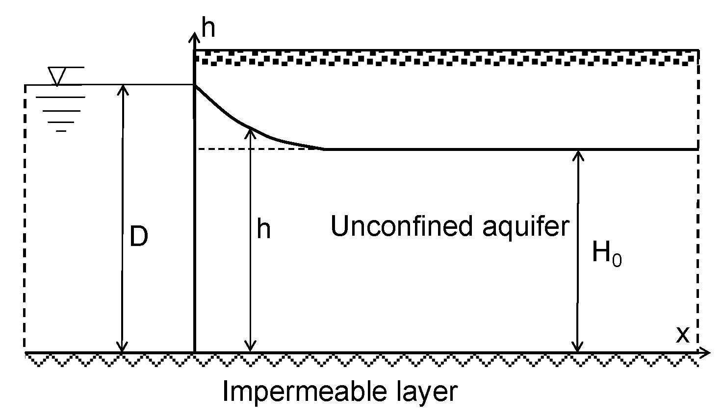
In the case of the aquifer illustrated in Figure 1, recharging from the lake, a rise in the water level of the lake is observed and the aquifer flow is described by the following Boussinesq equation:
or by its linear representation [13]:
In Equation (2), K = the hydraulic conductivity of the aquifer, S = the specific yield of the aquifer or drainable pore space, D = the depth of the lake, h(x,t) = the depth of the aquifer, and x,t = the coordinates (spatial and temporal). The boundary conditions of the problem are:
while the initial flow condition is:
To facilitate calculations non-dimensional variables are introduced:
where L = a specific length. The new resulting equation is as follows:
with the new boundary conditions:
and the initial flow condition:
Fuzzy Case
The fuzzy form of Equation (6) is:
with the new boundary and initial conditions:
where c = the spread and α = the α-cut.
2.2. Mathematical Model
2.2.1. Definitions
Definition 1.
A fuzzy seton a universe set X is a mapping , assigning to each element a degree of membership The membership function is also defined as with the properties:
(i)is upper semicontinuous, (ii) = 0, outside of some interval [c,d], (iii) there are real numbers , such that is monotonic nondecreasing on [c,a], monotonic nonincreasing on [b,d] and = 1 for each (iv) is a convex fuzzy set:
Definition 2.
Let X be a Banach space and be a fuzzy set on X. The α-cuts of are defined as
where cl(supp) denotes the closure of the support of .
Definition 3.
Let Ҡ(X) be the family of all nonempty compact convex subsets of a Banach space. A fuzzy set on X is called compact if Ҡ(X), The space of all compact and convex fuzzy sets on X is denoted as Ƒ (X).
Definition 4.
Let RƑ. The α-cuts of , are: . According to representation theorem of [36] and the theorem of [37], the membership function and the α-cut form of a fuzzy number , are equivalent and in particular the α-cuts uniquely represent , provided that the two functions are monotonic ( monotonic nondecreasing, monotonic nonincreasing) and
Definition 5.
gH-Differentiability [34,38]. Let RƑ be such that . Suppose that the functions and are real-valued functions, differentiable w.r.t. x, uniformly w.r.t. . Subsequently, the function is gH-differentiable at a fixed if and only if one of the following two cases holds:
is increasing,is decreasing as functions of α, and , or
is increasing,is decreasing as functions of α, and .
Notation1:. In both of the above cases,derivative is a fuzzy number.
Notation2: The first case concerns the Hukuhara differentiability.
Definition 6.
• is (i)-gH-differentiable at x0 if
• (ii)-gH-differentiable at x0 if
Definition 7.
g-differentiability. Let RF be such that . If and are differentiable real-valued functions with respect to x, uniformly for , then is g-differentiable [38]:
Definition 8.
The gH-differentiability implies g-differentiability, but the inverse is not true.
Definition 9.
[gH-p] differentiability. A fuzzy-valued function of two variables is a rule that assigns to each ordered pair of real numbers (x, t), in a set Dxt a unique fuzzy number denoted by . Let : Dxt RƑ, (x0, t0) Dxt and , : are real valued functions and partial differentiable w.r.t. x. [35,39,40]:
is [(i)-p]-differentiable w.r.t. x at (x0, t0) if:
is [(ii)-p]-differentiable w.r.t. x at (x0, t0) if:
Notation. The same is valid for.
2.2.2. Transform of the Fuzzy Problem
Systems of Crisp Problems
Our problem is transformed now to the following fuzzy partial differential equation:
with the new boundary and initial conditions:
Solutions to the fuzzy problem (20) with the boundary and initial conditions (21), utilizing the theory of [35,38,39,41] can be found, translating the above fuzzy problem to a system of second order of crisp boundary value problems, hereafter called corresponding system for the fuzzy problem. Therefore, four crisp BVPs systems are possible for the fuzzy problem, as follows:
(1.1)-system:
(1.2)-system:
(2.1)-system:
(2.2)-system:
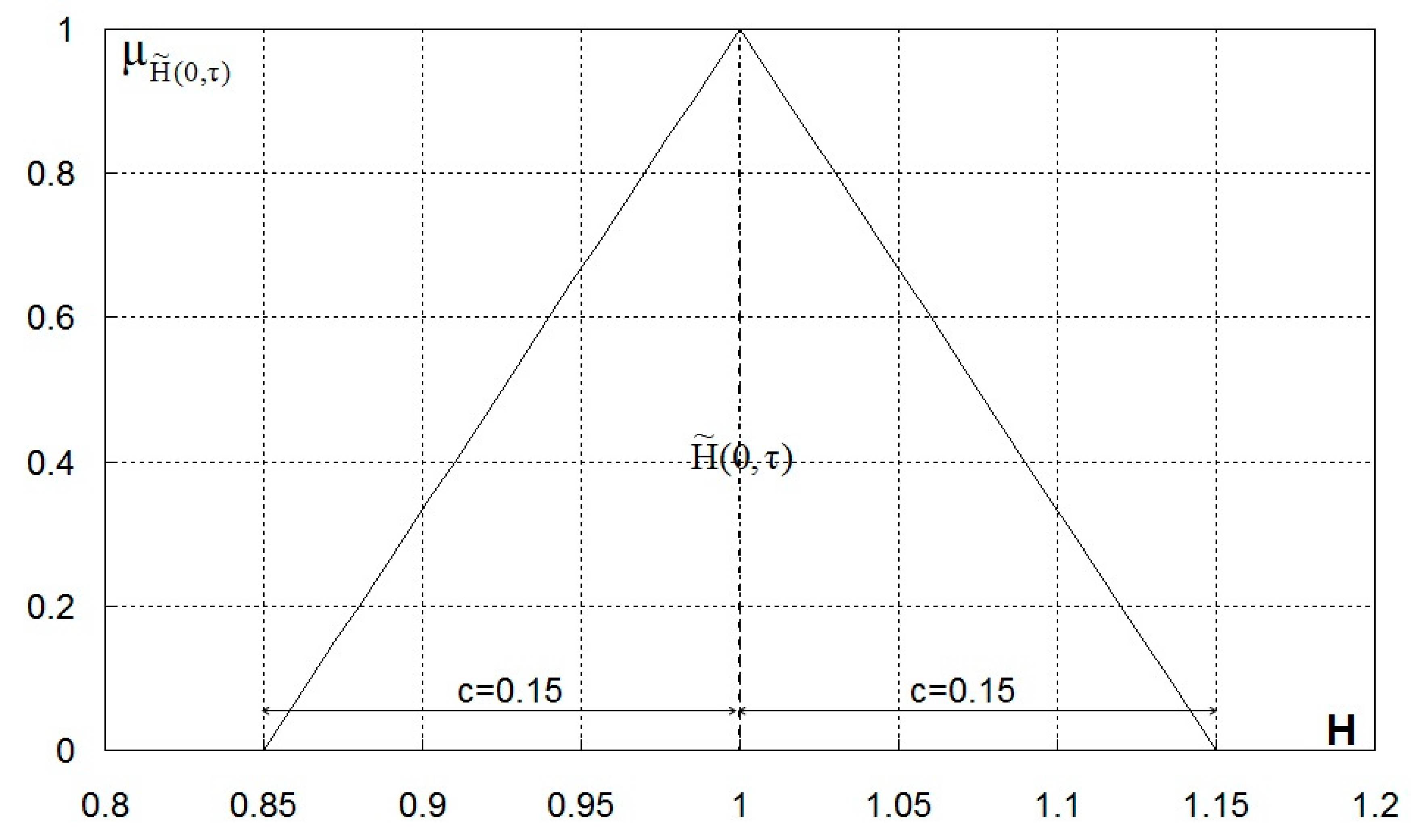
Figure 2 illustrates the fuzzy boundary condition
The method of solving the above problem is based on the selection of appropriate type of derivative, according to the theory of [38,39]. With such a selection, the above problem is transformed to a corresponding system of boundary value problems. A domain with the valid solution results, in which the derivatives have level sets according to the above theory of differentiability.
2.2.3. Solution of the (1.1)-System
Let now , and . Subsequently, the above system becomes:
First Equation of (1.1)
The Boltzmann transform is introduced now in Equation (22):
Equation (22) takes the following form:
with boundary conditions:
The solution is:
Based on Equation (26) the following arise:
Second Equation of (1.1)
According to the same procedure as above:
Based now on Equation (30) the following arises:
The final solution of the system is:
This solution satisfies the system (1,1), as well as the boundary and initial conditions of the system.
The first derivatives with respect to τ are the following,
and form a fuzzy number as:
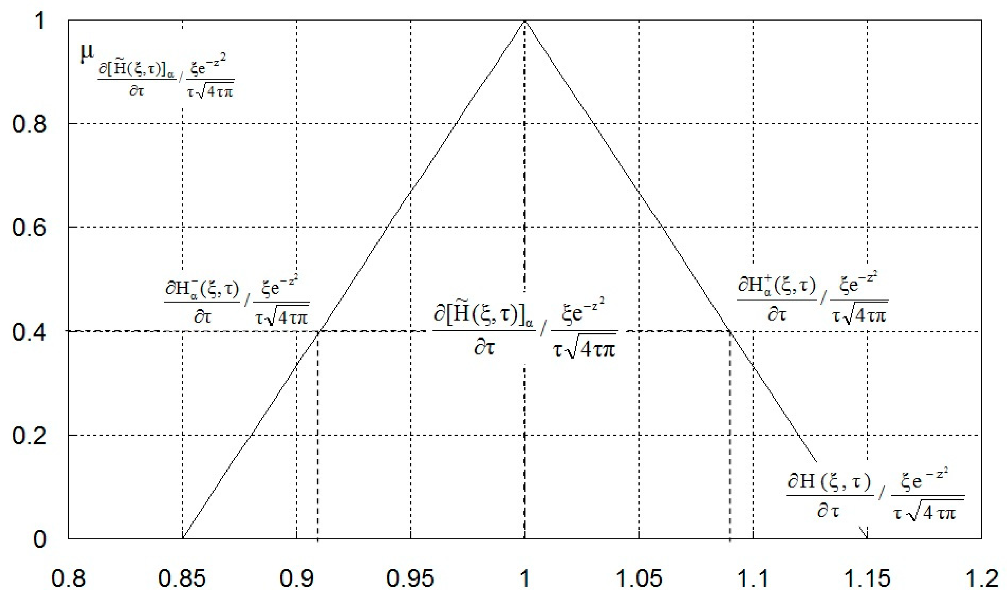
Figure 3 illustrates the first derivative with respect to τ.
The second derivatives with respect to ξ are the following:
and form a fuzzy number as:
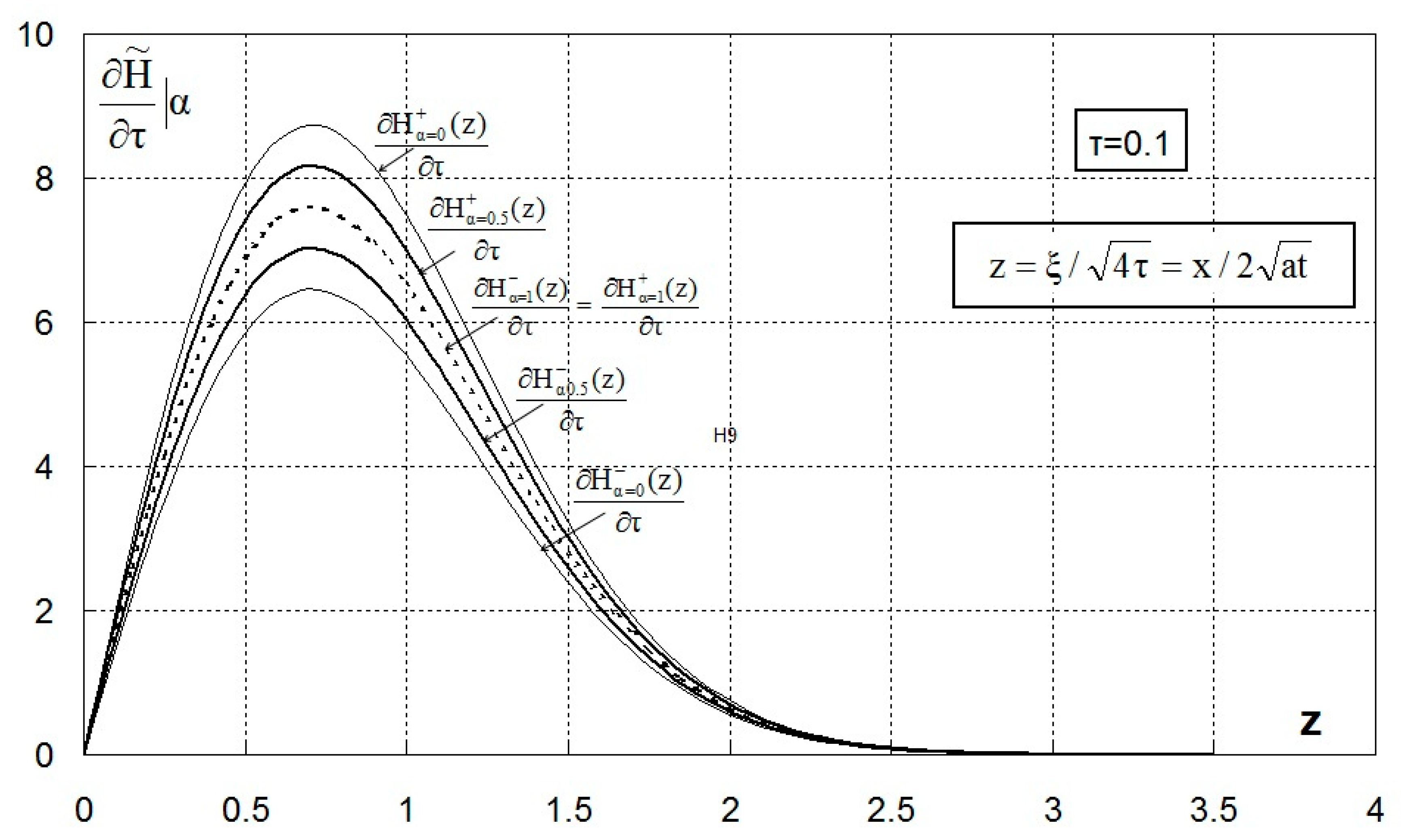
Figure 4 illustrates the change of the derivative with respect to z, for α = 0, 0.5 and 1.
From Equations (34) and (36), the following results:
Boundaries condition
Initial condition
2.2.4. Solution of the (1.2)-System
are introduced and the above system takes the form:
Solution
Adding the two equations:
Let now: , so the above equation becomes:
and the solution is:
The difference of the two equations is taken and it results to:
Writing now: , the above equation becomes:
The solution of the new equation is obtained by introducing Boltzmann transformation . The new equation is:
with the new boundary conditions
The solution of the above Equation (44) is:
Introducing now the boundary conditions formulated by (45):
where the function f(z) is equal to:
Figure 5 illustrates the function f(z) with respect to z.
Note: the above integral is given, as follows [42]:
The form of the function f(z) is indicative, since for the calculation of the above series, 43 terms were taken and the convergence criterion is:
The solution of the system is:
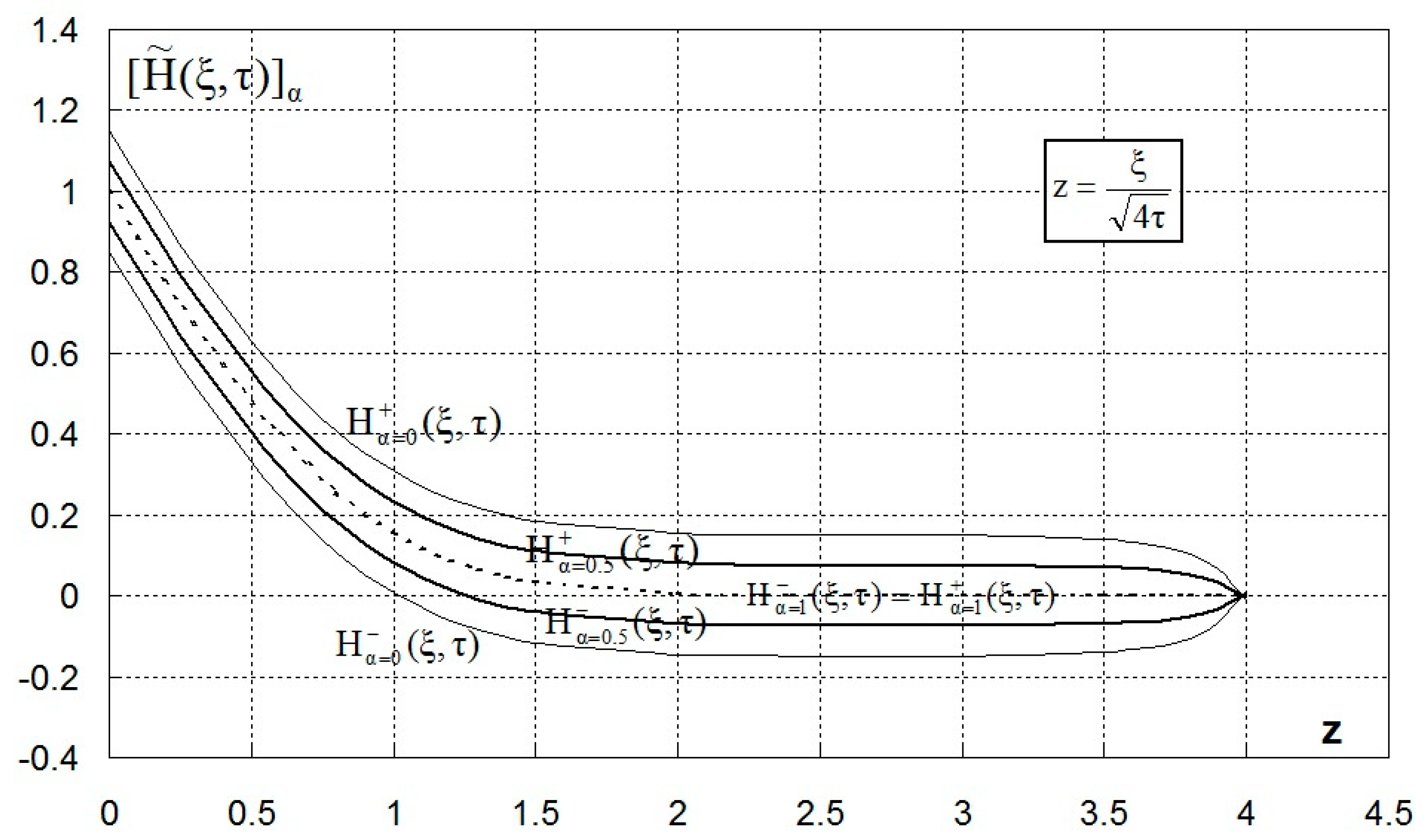
In the above solution an indicative value for z = 4 was selected and in Figure 6 it is shown that after the value z = 1.017, negative values of the function for α = 0, 0.5 appear. This means that for the physical problem this solution is not acceptable for z > 1.017.
The first derivative w.r.t. τ
The following results to:
The second_derivative w.r.t. ξ
The following results to:
The first derivative with respect to τ is a fuzzy number and the second derivative with respect to ξ is also a fuzzy number according the theory of [38]. The above system (1.2) satisfies the Equation (38) as well as the initial and boundary conditions and has fuzzy derivatives. The solution for the physical problem is valid only for
2.2.5. Solution of the (2.1)-System
It is proved that the solution of the system (2.1) is similar to the solution of system (1.2)
2.2.6. Solution of the (2.2)-System
It is proved that the solution of the system (2.2) is similar to the solution of system (1.1).
2.2.7. Darcy Velocity, Water Flow Recharging Volume
The Darcy’s velocity is:
The partial derivative is equal to: and the following expression arises:
The real velocity is equal to:
Introducing dimensionless velocity:
The volume recharging from the lake will be:
The dimensionless volume is introduced:
3. Results and Discussion
3.1. Parameters of the Problem
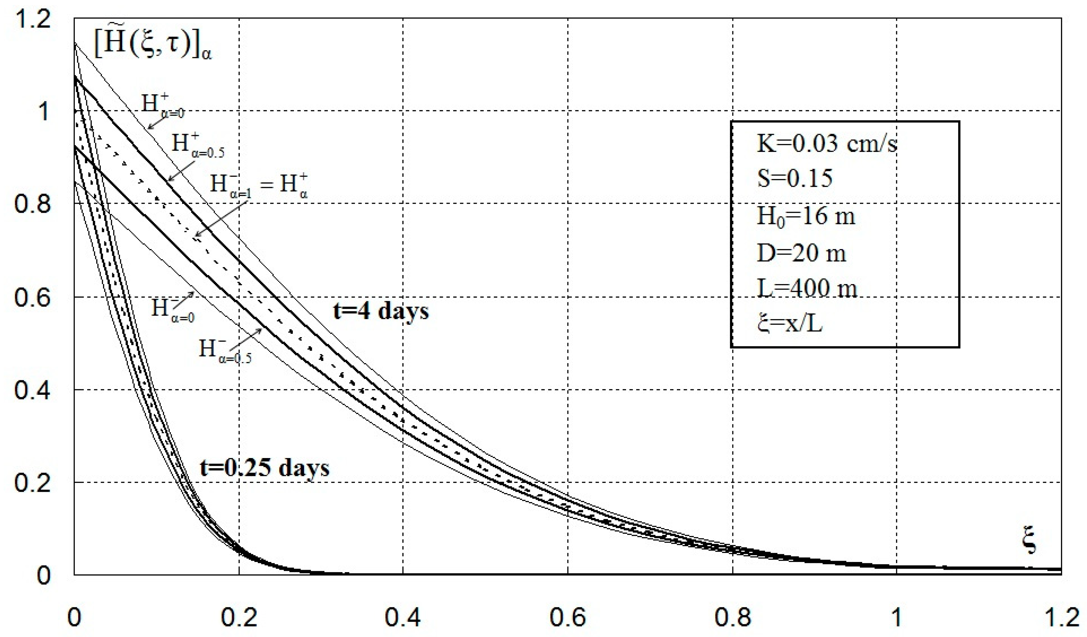
For the aquifer of Figure 1, the following are assumed: K = 0.03 cm/s (gravelly coarse sand [13]), S = 0.15, D = 20 m, H0 = 16 m, L = 400 m. Fuzziness is introduced on (c = 0.15), that is:
and the solution becomes:
Note: The cases (1.1) and (2.2) are considered here, since they give a physical solution to the problem of aquifer recharging from the lake. In the following, the Darcy velocity and the recharging volume of the aquifer are presented.
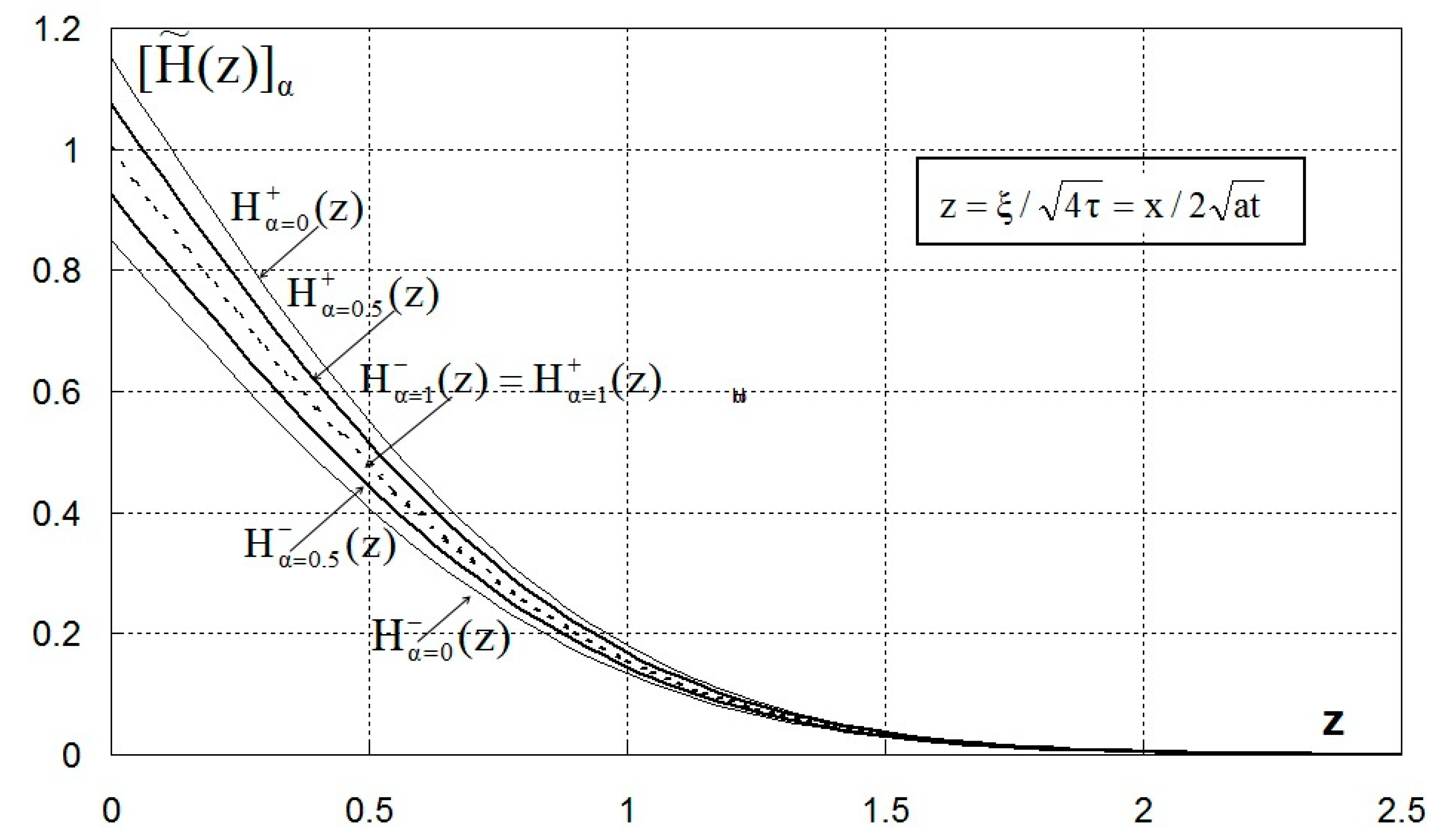
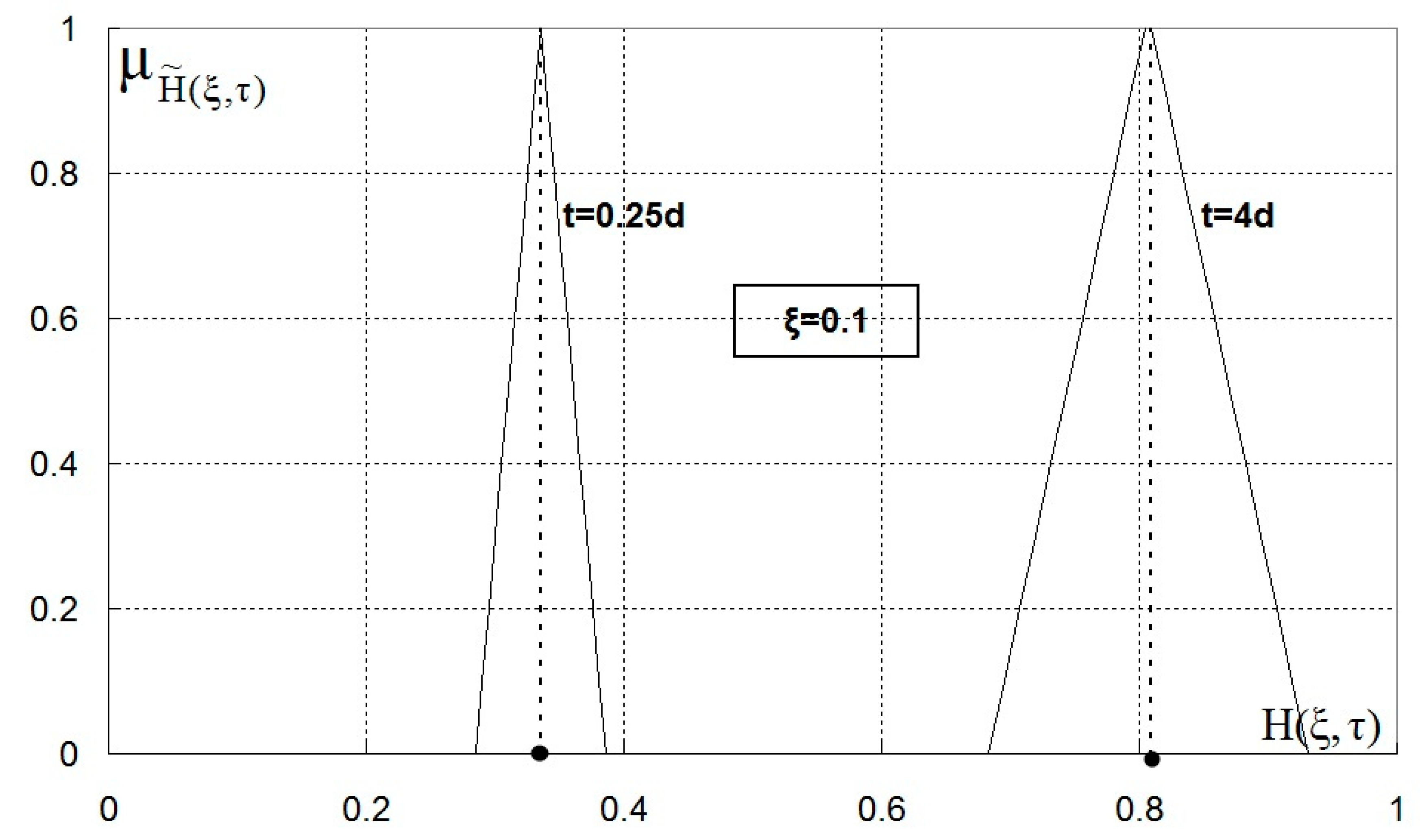
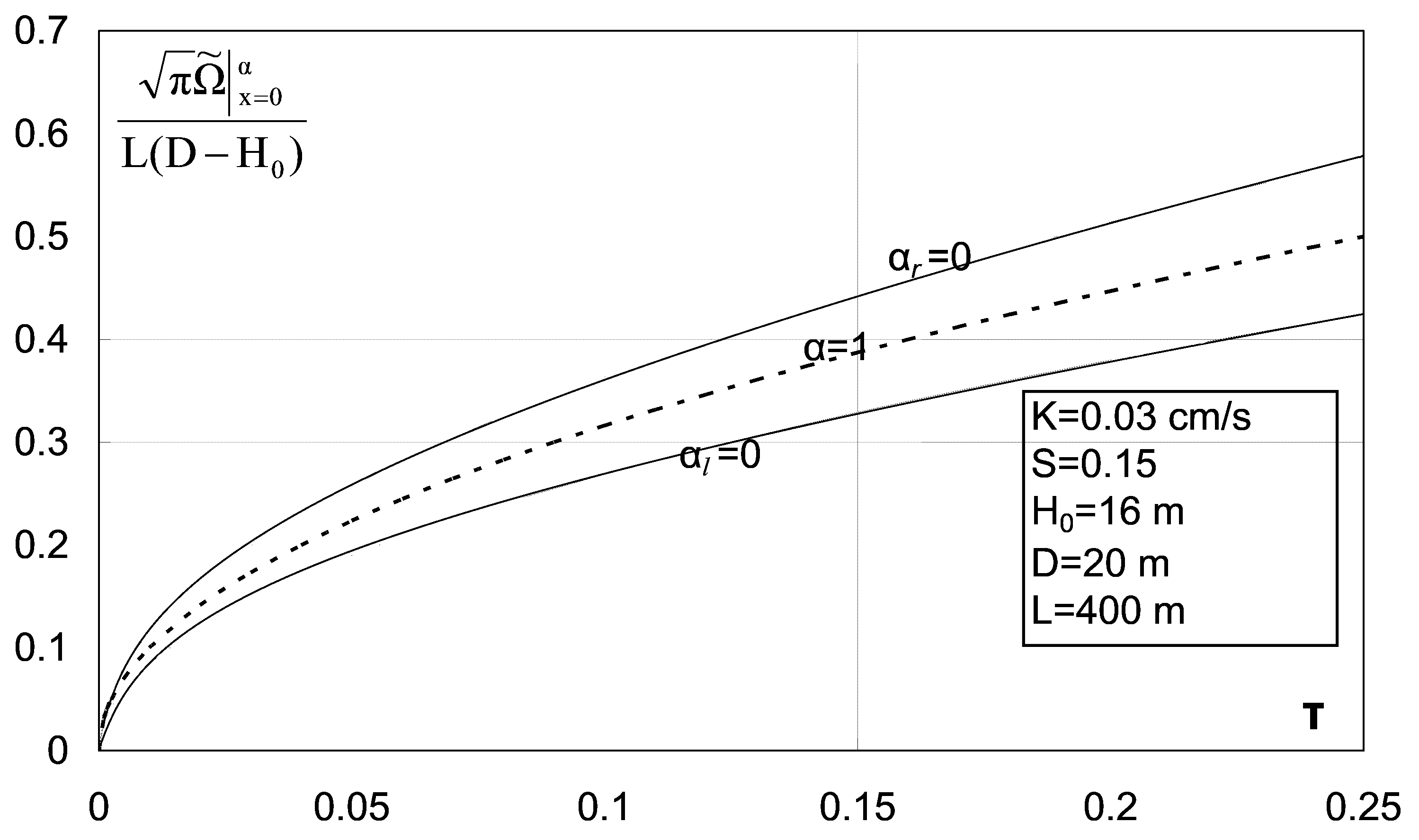
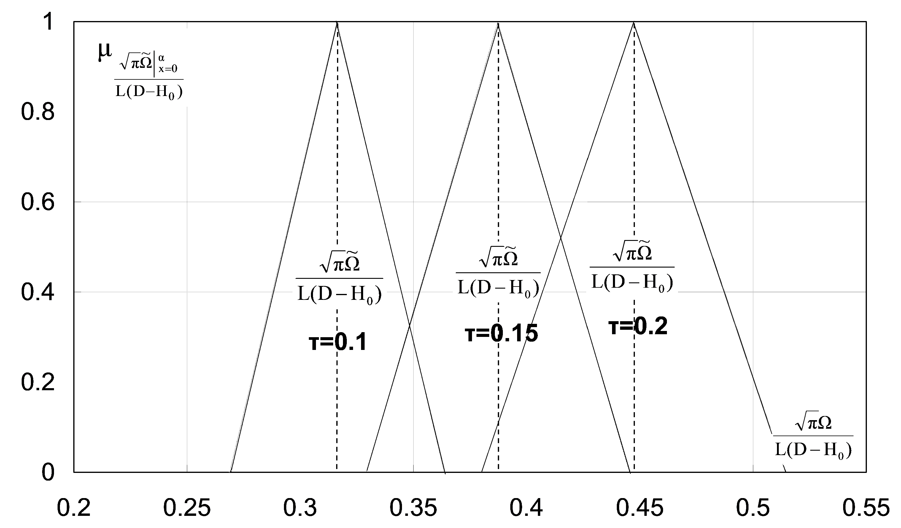
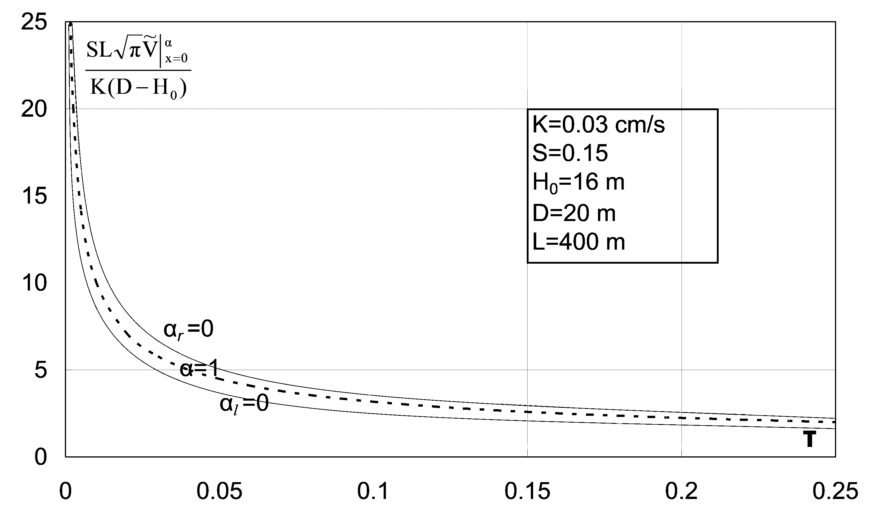
In Figure 7, the change in dimensionless depth is presented as a function of z, while Figure 8 illustrates dimensionless depth profiles as a function of ξ, for times t = 0.25 d, and 4d. Figure 9 illustrates membership functions at ξ = 0.1, for times t = 0.25 d, and 4 d. Figure 7, shows that the waterfront towards the aquifer approaches the position z = 2.125. That front corresponds in real times t ~ 0.25 d, and 4 d, at distances 125 m, 500 m apart from the lake. Figure 10, illustrates the recharging water volume at x = 0, while Figure 11 illustrates the membership function for times τ = 0.1, 0.15, and 0.2. Finally, Figure 12 illustrates the real dimensionless velocity versus dimensionless time τ. The water volumes that are depicted in Figure 10 for an aquifer width of 2000 m, are the following:
- t1 = 4.63 d( = 485,281 m3 ± 85,638 m3),
- t2 = 6.94 d( = 594346 m3 ± 104,884 m3),
- t3 = 9.26 d ( = 682,292 m3 ± 121,110 m3).
3.2. Remark
Many times we try to find the difference using trapezoidal or Gaussian membership functions. Here, some explanations concerning the above cases are given.
3.2.1. Trapezoidal Membership Function
A symmetrical trapezoidal membership function with the same fuzziness c and a core equal to is considered. Subsequently, the boundary and initial conditions of the problem will be:
and the solution will be:
(a) This solution with converges to the solution with a triangular membership function.
(b) For cases where the core width (2ε) is large enough, the solution with a trapezoidal membership function will give a cut larger than the present solution with triangular membership function.
3.2.2. Gaussian Membership Function
First a fuzzy Gaussian number is considered as follows: .
Afterwards, a triangular fuzzy number is selected with membership function and having the following properties:
The base of triangular fuzzy number is equal to: . In reference [43] it is proved that in this way the two membership functions almost coincide. Accordingly, using this method that transforms the Gaussian number to triangular one, it is proved that, when using the Gaussian membership function, the results remain the same.
3.3. Remark Concerning the Uncertainties of the Parameters
In this analysis, the focus was on the ambiguity of the initial conditions of the problem. It should be stressed, of course, that ambiguity is introduced into a linearized Boussinesq equation, which can provide information on solving the non-linear equation of Boussinesq by numerical methods. Also, there are more possible ambiguities on the parameters of hydraulic conductivity and effective porosity, since they are measurable quantities. The effect of these ambiguities should be considered and included for future research.
4. Conclusions
The [32] theory with the generalized Hukuhara (g-H) derivative, as well as its extension by [38] to partial differential equations, allows researchers to solve practical problems, which is useful in engineering. It is now possible for engineers to take the fuzziness of various sizes involved into consideration when calculating and making a decision on their work.
Boussinesq’s linear equation regarding the aquifer case study has a fuzzy solution that is unique, and the function is [(ii)-p] differentiable with respect to ξ and [(i)-pp] with respect to τ. The function is [(ii)-p] differentiable with respect to ξ.
The fuzzy water volume variations (spreads) regarding their average value, amount to 15% of the average values of all times, and therefore, equal to the initial relative fuzziness in boundary values. The fuzzy water flow velocity tends asymptotically to zero, while the recharging fuzzy water volume tends asymptotically to infinity.
It is important here to note, that for practical cases (artificial recharge problem, irrigation, and drainage projects), the engineers should take the right decision, knowing the deviations of the crisp value of water volume from the fuzzy ones, which here attains 15%.
Using trapezoidal membership functions, the difference is negligible if the core width is small. For larger values of core width, α-cuts intervals that are larger than the present solution arise. Using the Gaussian membership function, the results remain the same.
Author Contributions
C.T. conceived the whole idea and gave the solution of the (1,1) system and (1,2) systems; K.P. gave the solution of (2,2) system; C.E. gave the solution of (2,1) system; B.P. revised the paper.
Conflicts of Interest
The authors declare no conflict of interest.
References
- Boussinesq, J. Recherches théoriques sur l’écoulement des nappes d’eau infiltrées dans le sol et sur le débit des sources. J. Math. Pures Appl. 1904, 10, 5–78. [Google Scholar]
- Polubarinova-Cochina, P.Y. On unsteady motions of groundwater during seepage from water reservoirs. P.M.M. (Prinkladaya Matematica I Mekhanica) 1949, 13, 2. [Google Scholar]
- Werner, P.W. On non-artesian groundwater flow. Geofis. Pura Appl. 1953, 25, 37–43. [Google Scholar] [CrossRef]
- Dumm, L.D. New formula for determining depth and spacing of subsurface drains in irrigated lands. Agric. Eng. 1954, 35, 726–730. [Google Scholar]
- Dumm, L.D. Validity and use of the transient flow concept in subsurface drainage. Paper No 60-717 Presented at Asae Meeting, Memphis, TN, USA, 4–7 December 1960; pp. 4–7. [Google Scholar]
- Maasland, M. Water Table Fluctuations Induced by Intermittent Recharge. J. Geophys. Res. 1959, 64, 549–559. [Google Scholar] [CrossRef]
- Van Schilfgaarde, J.; Kirkham, D.; Frevert, R.K. Physical and Mathematical Theories Of Tile and Ditch Drainage And Their Usefulness in Design. In Research Bulletin 436; Agricultural Experiment Station, Iowa State College: Ames, IA, USA, 1956. [Google Scholar]
- Polubarinova-Cochina, P.Y. On a non-linear differential equation occurring in seepage theory. DAN 1948, 36, 82. [Google Scholar]
- Polubarinova-Cochina, P.Y. Theory of Groundwater Movement, 2015th ed.; Princeton University Press: Princeton, NJ, USA, 2015; p. 613. [Google Scholar]
- Aravin, V.I.; Numerov, S.N. Theory of Fluid Flow in Deformable Porous Media; Israel Program for Scientific Translation: Jerusalem, Israel, 1965; p. 511. [Google Scholar]
- Glover, R.E. Transient Groundwater Hydraulics, 2nd ed.; Water Resources Publications LLC: Fordt Collins, CO, USA, 1978; p. 413. [Google Scholar]
- Hálek, V.; Švek, J. Ground Water Hydraulics, 1979th ed.; Elsevier Scientific Publishing Company: Amsterdam, The Netherlands; Oxford, UK, 1979; p. 620. [Google Scholar]
- De Ridder, N.A.; Zijlstra, G. Seepage and Groundwater Flow. In Drainage Principles and Applications, 2nd ed.; Ritzema, H.P., Ed.; ILRI Publication 16: Wageningen, The Netherlands, 1994; pp. 305–340. [Google Scholar]
- Serrano, S.E.; Workman, S.R.; Srivastava, K.; Miller-Van Cleave, B. Models of nonlinear stream aquifer transients. J. Hydrol. 2007, 336, 199–205. [Google Scholar] [CrossRef]
- Parlange, J.-Y.; Hogarth, W.L.; Govindaraju, R.S.; Parlange, M.B.; Lockington, D. On an Exact Analytical Solution of the Boussinesq Equation. Transp. Porous Media 2000, 39, 339–345. [Google Scholar] [CrossRef] [Green Version]
- Srivastava, K.; Serrano, S.E.; Workman, S.R. Stochastic modelling of transient stream–aquifer interaction with the nonlinear Boussinesq equation. J. Hydrol. 2006, 328, 538–547. [Google Scholar] [CrossRef]
- Serrano, S.; Workman, S.R. Modeling transient stream/aquifer interaction with the non-linear Boussinesq equation and its analytical solution. J. Hydrol. 1998, 206, 245–255. [Google Scholar] [CrossRef]
- Aminikhah, H. Approximate analytical solution for the one-dimensional nonlinear Boussinesq equation. Int. J. Numer. Method Heat 2015, 25, 831–840. [Google Scholar] [CrossRef]
- Zadeh, L.A. Fuzzy Sets. Inf. Control 1965, 8, 338–353. [Google Scholar] [CrossRef]
- Bhaskar, T.; Lakshmikantham, V.; Devi, V. Revisiting fuzzy differential equations. Nonlinear Anal. 2004, 58, 351–358. [Google Scholar] [CrossRef]
- Kaleva, O. A note on fuzzy differential equations. Nonlinear Anal. 2006, 64, 895–900. [Google Scholar] [CrossRef]
- Nieto, J.J.; Rodríguez-López, R. Bounded solutions for fuzzy differential and integral equations. Chaos Solitons Fractals 2006, 27, 1376–1386. [Google Scholar] [CrossRef]
- Guo, M.; Xue, X.; Li, R. The oscillation of delay differential inclusion and fuzzy biodynamics models. Math. Comput. Model. 2003, 37, 651–658. [Google Scholar] [CrossRef]
- Guo, M.; Xue, X.; Li, R. Impulsive functional differential inclusion and fuzzy population models. Fuzzy Sets Syst. 2003, 138, 601–615. [Google Scholar] [CrossRef]
- Puri, M.L.; Ralescu, D.A. Differentials of Fuzzy Functions. J. Math. Anal. Appl. 1983, 91, 552–558. [Google Scholar] [CrossRef]
- Hukuhara, M. Intégration des Applications Mesurables dont la Valeur est un Compact Convexe. Funkc. Ekvacioj 1967, 10, 205–233. [Google Scholar]
- Kaleva, O. Fuzzy differential equations. Fuzzy Sets Syst. 1987, 24, 301–317. [Google Scholar] [CrossRef]
- Seikkala, S. On the fuzzy initial problem. Fuzzy Sets Syst. 1987, 24, 319–330. [Google Scholar] [CrossRef]
- Vorobiev, D.; Seikkala, S. Towards the theory of fuzzy differential equations. Fuzzy Sets Syst. 2002, 125, 231–237. [Google Scholar] [CrossRef]
- O’Regan, D.; Lakshmikantham, V.; Nieto, J.J. Initial and boundary value problem for fuzzy differential equations. Nonlinear Anal. 2003, 54, 405–415. [Google Scholar] [CrossRef]
- Diamond, P. Brief note on the variation of constants formula for fuzzy differential equations. Fuzzy Sets Syst. 2002, 129, 65–71. [Google Scholar] [CrossRef]
- Bede, B.; Gal, S.G. Generalizations of the differentiability of fuzzy-number-valued functions with applications to fuzzy differential equations. Fuzzy Sets Syst. 2005, 151, 581–599. [Google Scholar] [CrossRef]
- Bede, B. A note on two-point boundary value problems associated with non-linear fuzzy differential equations. Fuzzy Sets Syst. 2006, 157, 986–989. [Google Scholar] [CrossRef]
- Stefanini, L. A generalization of Hukuhara difference and division for interval and fuzzy Arithmetic. Fuzzy Sets Syst. 2010, 161, 1564–1584. [Google Scholar] [CrossRef]
- Allahviranloo, T.; Gouyandeh, Z.; Armand, A.; Hasanoglu, A. On fuzzy solutions for heat equation based on generalized Hukuhara differentiability. Fuzzy Sets Syst. 2015, 265, 1–23. [Google Scholar] [CrossRef]
- Negoita, C.V.; Ralescu, D.A. Representation theorems for fuzzy concepts. Kybernetes 1975, 4, 169–174. [Google Scholar] [CrossRef]
- Goetschel, R.; Voxman, W. Elementary fuzzy calculus. Fuzzy Sets Syst. 1986, 18, 31–43. [Google Scholar] [CrossRef]
- Bede, B.; Stefanini, L. Generalized differentiability of fuzzy-valued functions. Fuzzy Sets Syst. 2013, 230, 119–141. [Google Scholar] [CrossRef]
- Khastan, A.; Nieto, J.J. A boundary value problem for second order fuzzy differential equations. Nonlinear Anal. 2010, 72, 3583–3593. [Google Scholar] [CrossRef]
- Mondal, S.P.; Roy, T.K. Solution of second order linear differential equation in fuzzy Environment. Ann. Fuzzy Math. Inform. 2015, x, 1–25. [Google Scholar]
- Bede, B.; Stefanini, L. Solution of Fuzzy Differential Equations with generalized differentiability using LU-parametric representation. In Proceedings of the 7th Conference of the European Society for Fuzzy Logic and Technology (EUSFLAT-11), Advances in Intelligent Systems Research, Aix-les-Bains, France, 18–22 July 2011; pp. 785–790. [Google Scholar] [CrossRef]
- Meyer zur Capellen, W. Integraltafeln: Sammlung unbestimmter Integrale elementarer Funktionen, 1950th ed.; Springer: Aachen, Germany, 1950; p. 292. [Google Scholar]
- Hanss, M.; Willner, K. On Using Fuzzy Arithmetic to Solve Problems with Uncertain Model Parameters. Int. J. Proj. Manag. 2000, 20, 1–8. [Google Scholar]
Figure 1.
Aquifer recharging from the lake.

Figure 2.
Fuzzy boundary condition

Figure 3.
First derivative with respect to τ.

Figure 4.
Change of the derivative with respect to z, for α = 0, 0.5 and 1.

Figure 5.
Function f(z) with respect to z.

Figure 6.
Variation of versus z.

Figure 7.
Dimensionless depth as a function of z for α = 0, 0.5, and 1.

Figure 8.
Dimensionless depth profiles as a function of ξ, for times t = 0.25 d and 4 d and for α = 0, 0.5, and 1.
Figure 8.
Dimensionless depth profiles as a function of ξ, for times t = 0.25 d and 4 d and for α = 0, 0.5, and 1.

Figure 9.
Membership function for t = 0.25 d, t = 4 d at ξ = 0.1.

Figure 10.
Recharging water volume at x = 0.

Figure 11.
Membership functions for times τ = 0.1, 0.15, and 0.2.

Figure 12.
The real dimensionless velocity versus dimensionless time τ.

© 2018 by the authors. Licensee MDPI, Basel, Switzerland. This article is an open access article distributed under the terms and conditions of the Creative Commons Attribution (CC BY) license (http://creativecommons.org/licenses/by/4.0/).
Share and Cite
MDPI and ACS Style
Tzimopoulos, C.; Papadopoulos, K.; Evangelides, C.; Papadopoulos, B. Fuzzy Solution to the Unconfined Aquifer Problem. Water 2019, 11, 54. https://doi.org/10.3390/w11010054
AMA Style
Tzimopoulos C, Papadopoulos K, Evangelides C, Papadopoulos B. Fuzzy Solution to the Unconfined Aquifer Problem. Water. 2019; 11(1):54. https://doi.org/10.3390/w11010054
Chicago/Turabian StyleTzimopoulos, Christos, Kyriakos Papadopoulos, Christos Evangelides, and Basil Papadopoulos. 2019. "Fuzzy Solution to the Unconfined Aquifer Problem" Water 11, no. 1: 54. https://doi.org/10.3390/w11010054
Note that from the first issue of 2016, this journal uses article numbers instead of page numbers. See further details here.