Relevance and Scale Dependence of Hydrological Changes in Glacierized Catchments: Insights from Historical Data Series in the Eastern Italian Alps

 ,
,  ,
,
Abstract
:1. Introduction
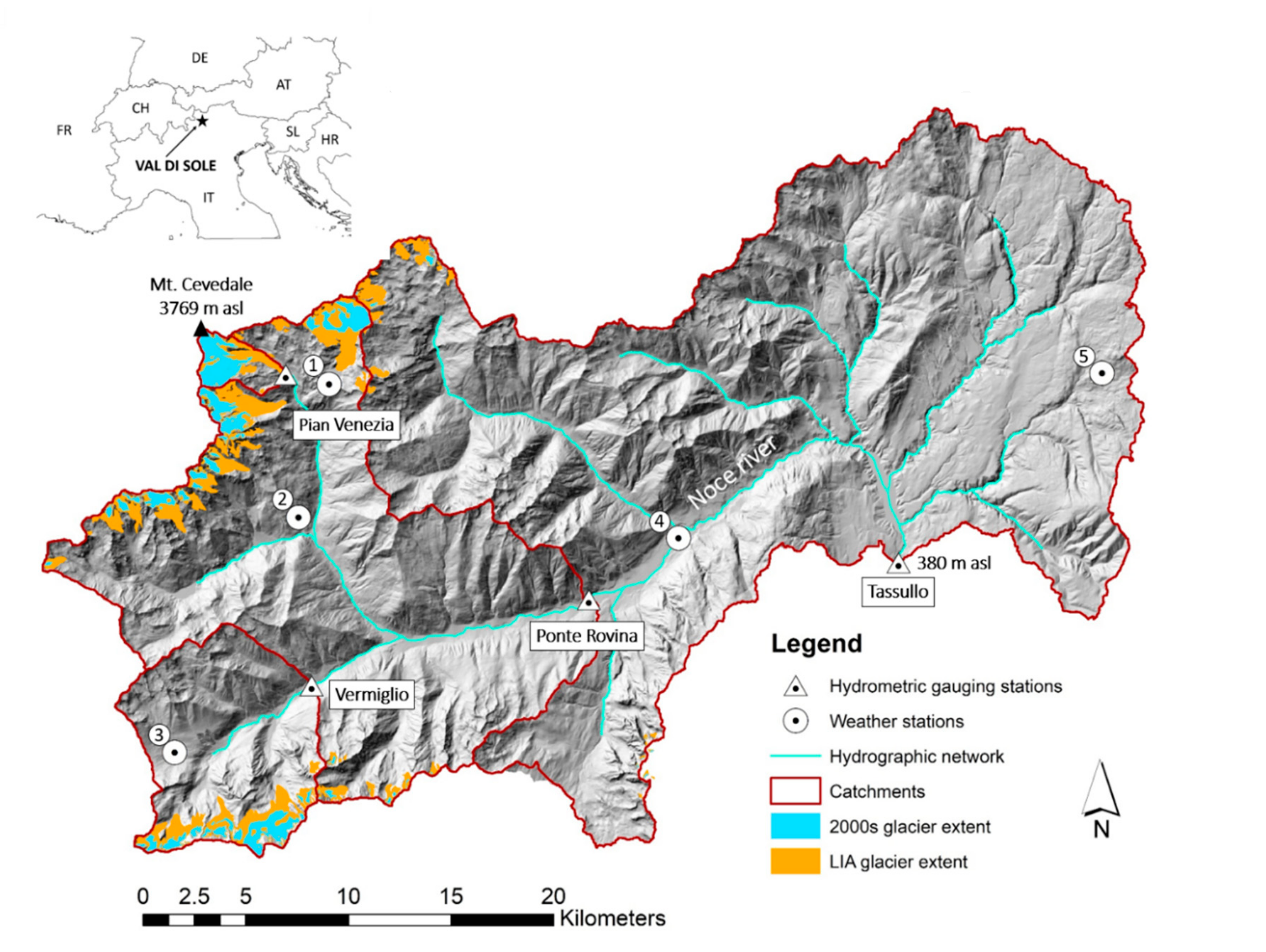
2. Study Area
3. Data Collection and Processing
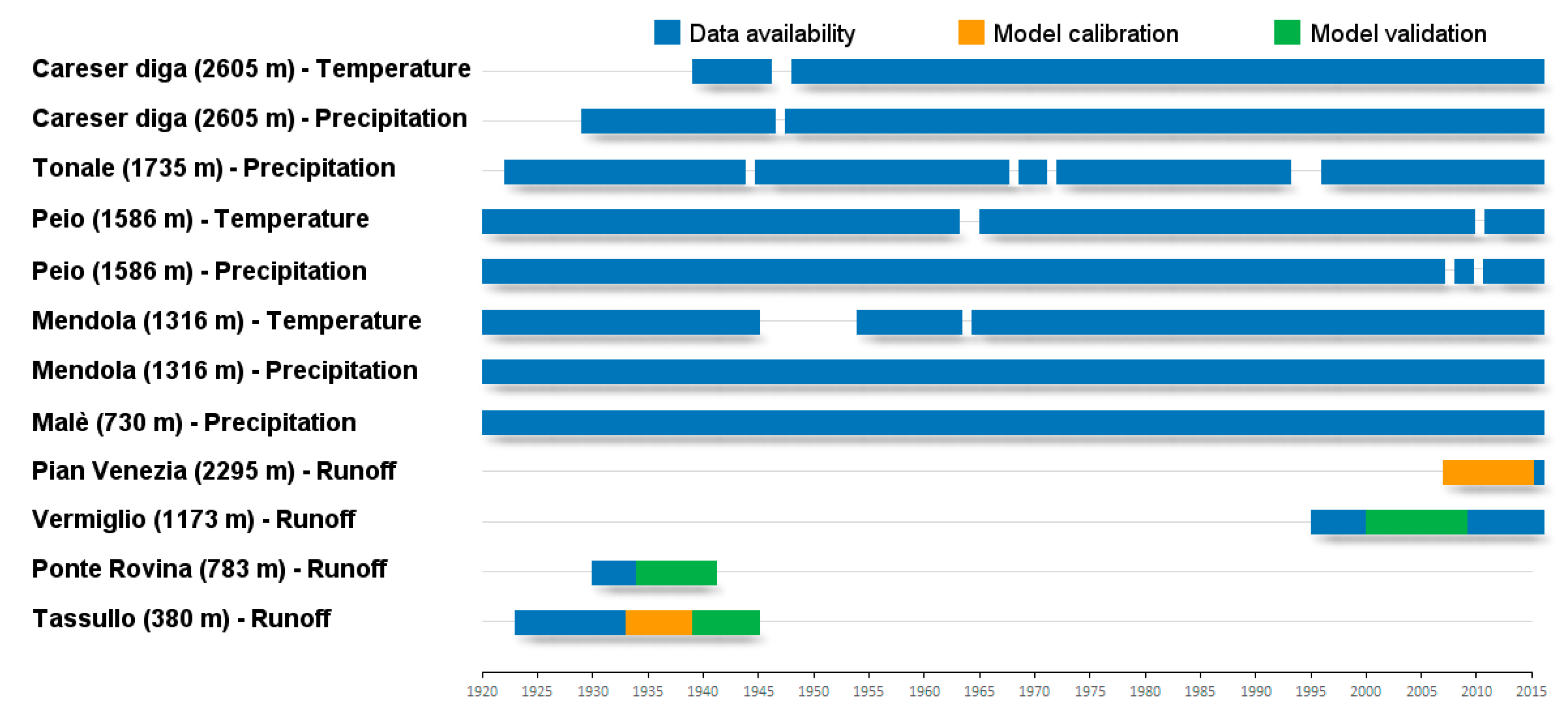
3.1. Hydro-Meteorological and Glacier Mass Balance Data
3.2. Glacier Extent and Topography
4. Sensitivity Analysis
4.1. Working Approach
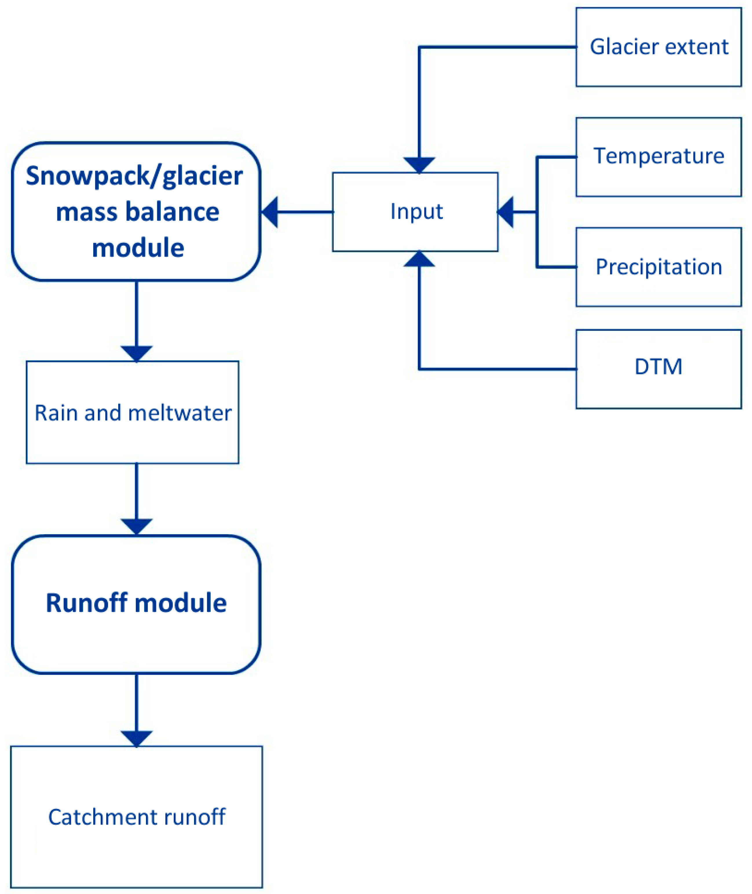
4.2. The Glacio-Hydrological Model
4.3. Model Calibration and Validation
5. Results
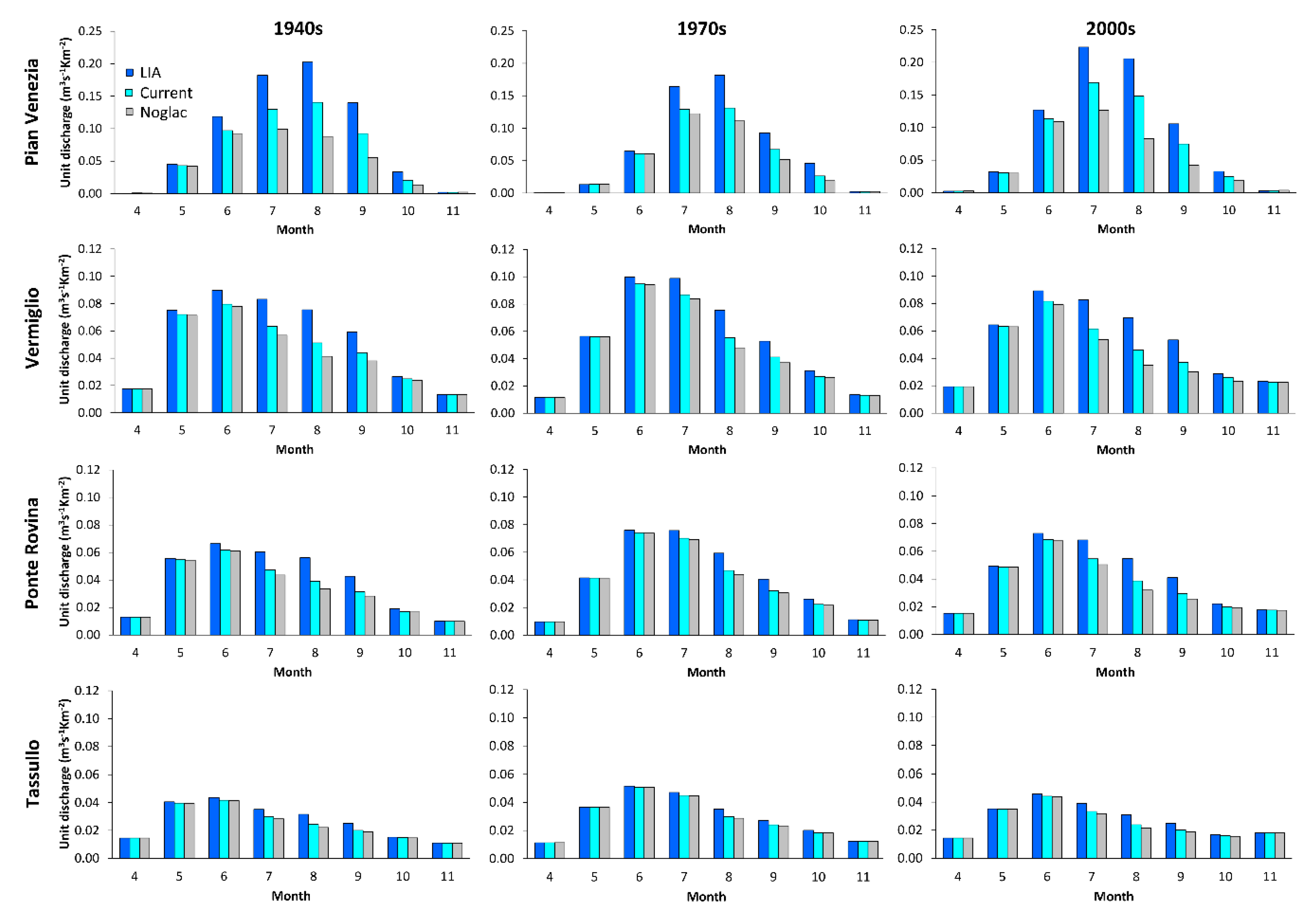
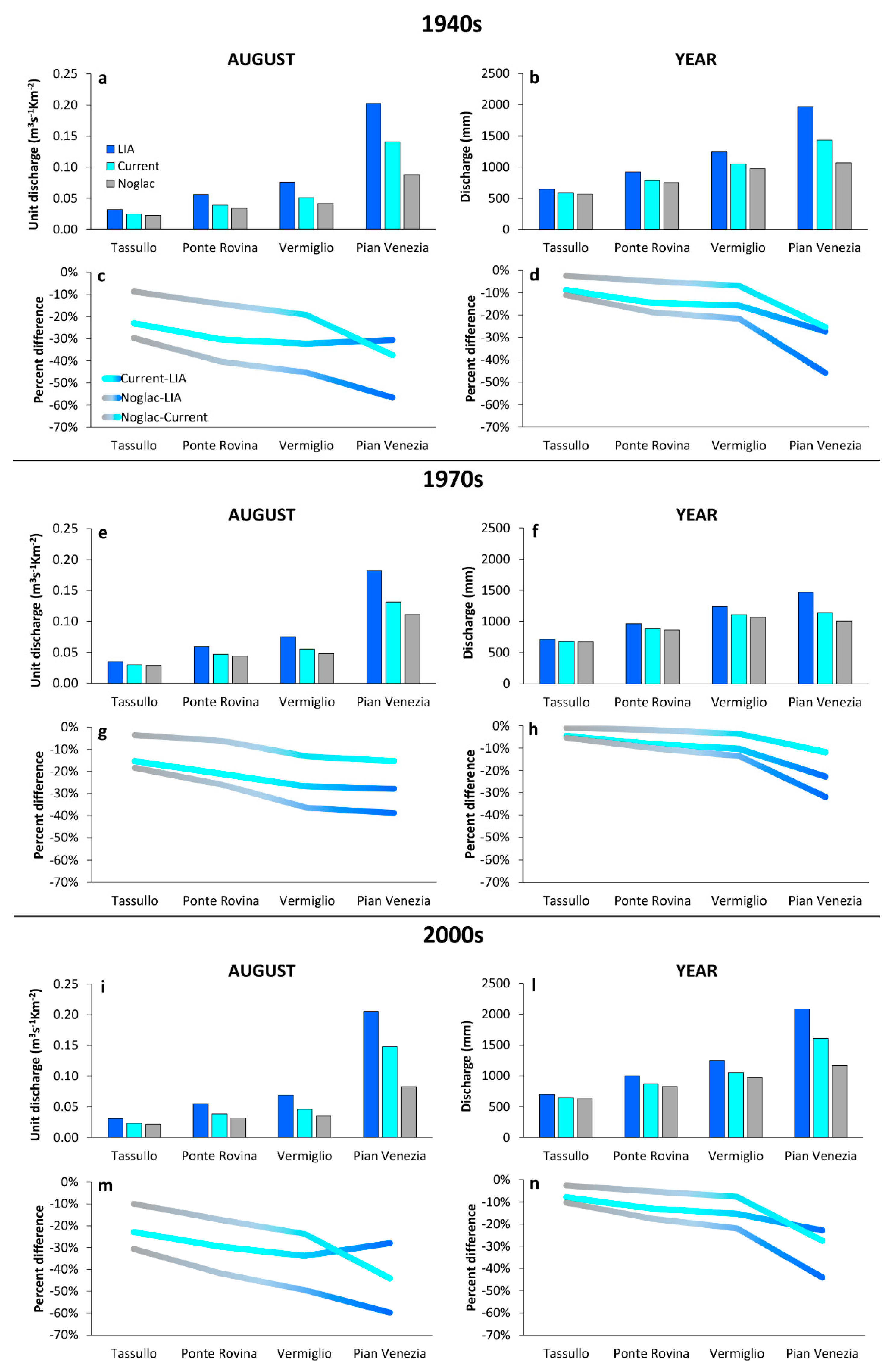
5.1. Runoff Regime under Different Meteorological Periods and Glacier Extent
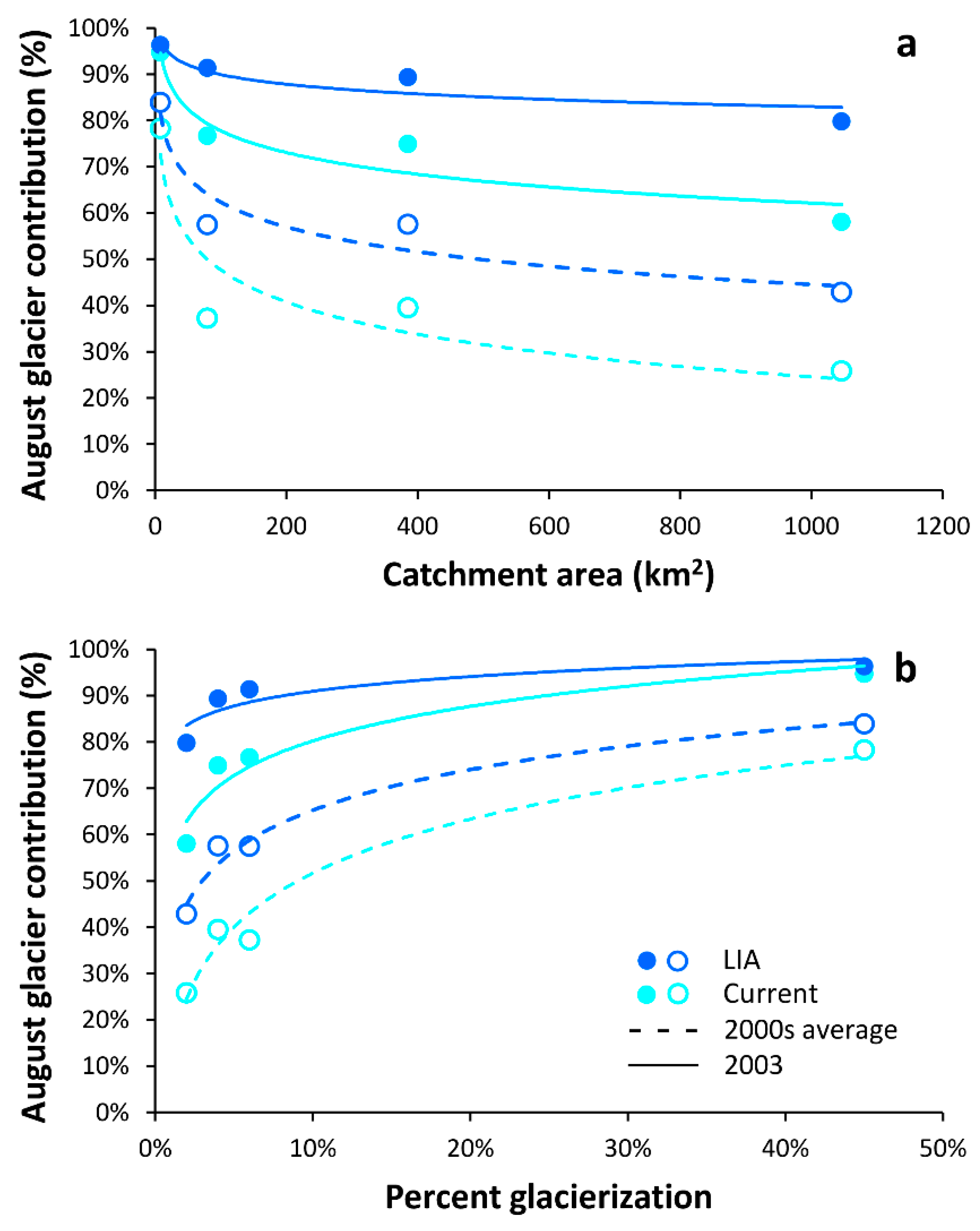
5.2. Scale Dependence of Hydrological Changes
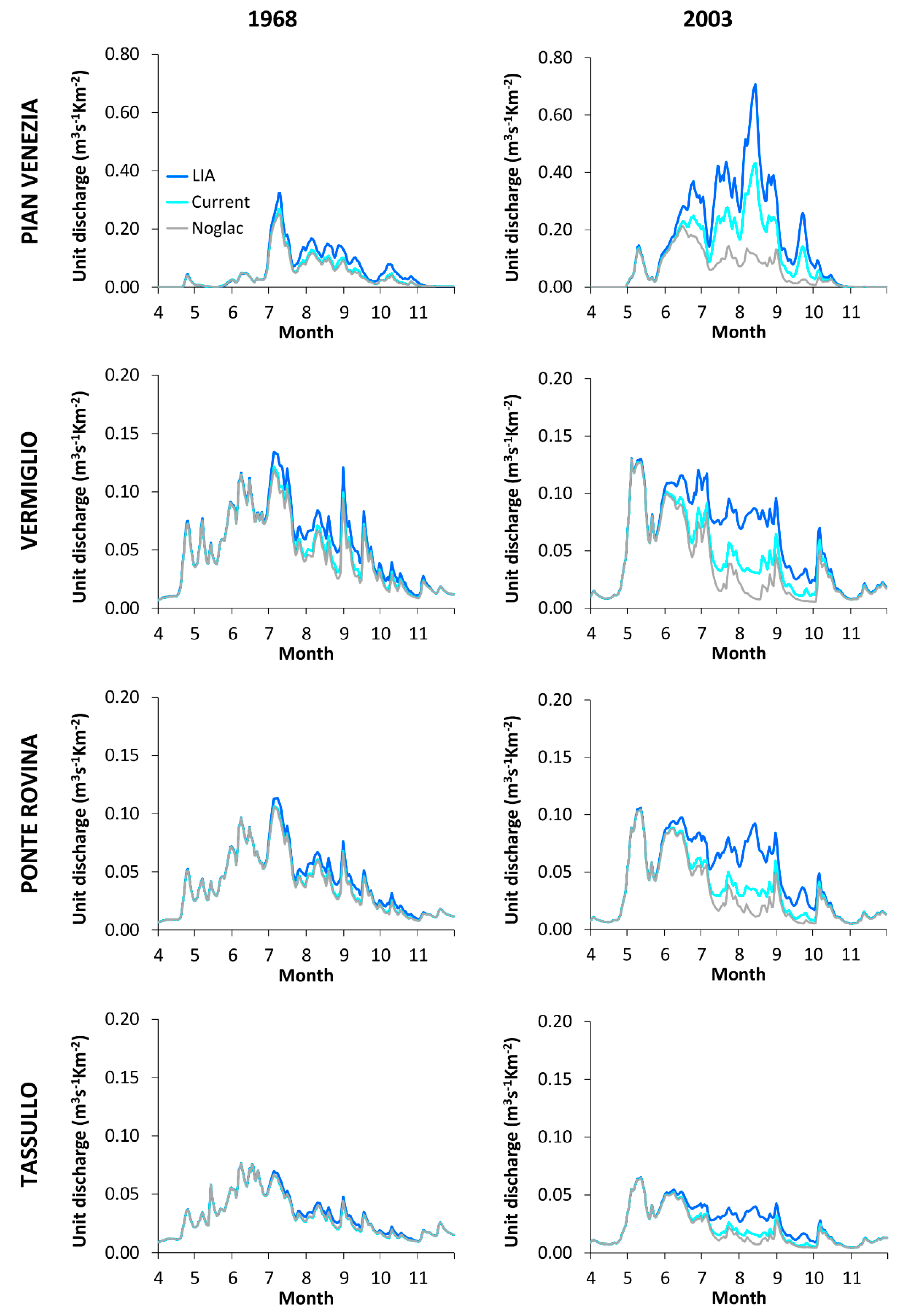
5.3. Hydrological Response under Extreme Meteorological Conditions
5.3.1. The 2003 Hydrological Year
5.3.2. The 1968 Hydrological Year
6. Discussion
6.1. Methodological Considerations
6.2. Considerations on the Sensitivity Analysis Results
7. Conclusions
Author Contributions
Funding
Acknowledgments
Conflicts of Interest
References
- Paul, F.; Kääb, A.; Maisch, M.; Kellenberger, T.; Haeberli, W. Rapid disintegration of Alpine glaciers observed with satellite data. Geophys Res Lett. 2004, 31, 12–15. [Google Scholar] [CrossRef]
- Zemp, M.; Haeberli, W.; Hoelzle, M.; Paul, F. Alpine glaciers to disappear within decades? Geophys Res Lett. 2006, 33, 6–9. [Google Scholar] [CrossRef]
- Zemp, M.; Frey, H.; Gärtner-Roer, I.; Nussbaumer, S.U.; Hoelzle, M.; Paul, F.; Haeberli, W.; Denzinger, F.; Ahlstrøm, A.P.; Anderson, B.; et al. Historically unprecedented global glacier decline in the early 21st century. J. Glaciol. 2015, 61, 745–762. [Google Scholar] [CrossRef] [Green Version]
- Haslinger, K.; Schöner, W.; Anders, I. Future drought probabilities in the Greater Alpine Region based on COSMO-CLM experiments—Spatial patterns and driving forces. Meteorol Z. 2015, 25, 137–148. [Google Scholar] [CrossRef]
- Huss, M. Present and future contribution of glacier storage change to runoff from macroscale drainage basins in Europe. Water Resour Res. 2011, 47, 1–14. [Google Scholar] [CrossRef]
- Junghans, N.; Cullmann, J.; Huss, M. Evaluating the effect of snow and ice melt in an Alpine headwater catchment and further downstream in the River Rhine. Hydrol Sci. J. 2011, 56, 981–993. [Google Scholar] [CrossRef] [Green Version]
- Farinotti, D.; Usselmann, S.; Huss, M.; Bauder, A.; Funk, M. Runoff evolution in the Swiss Alps: Projections for selected high-alpine catchments based on ENSEMBLES scenarios. Hydrol Process. 2012, 26, 1909–1924. [Google Scholar] [CrossRef]
- Majone, B.; Villa, F.; Deidda, R.; Bellin, A. Impact of climate change and water use policies on hydropower potential in the south-eastern Alpine region. Sci. Total Environ. 2016, 543, 965–980. [Google Scholar] [CrossRef]
- Koboltschnig, G.R.; Schöner, W. The relevance of glacier melt in the water cycle of the Alps: The example of Austria. Hydrol. Earth Syst. Sci. 2011, 15, 2039–2048. [Google Scholar] [CrossRef]
- Pelto, M.S. Skykomish River, Washington: Impact of ongoing glacier retreat on streamflow. Hydrol. Process. 2011, 25, 3267–3371. [Google Scholar] [CrossRef]
- Bliss, A.; Hock, R.; Radic, V. Global response of glacier runoff to twenty-first century climate change. J. Geophys. Res. Earth 2014, 119, 717–730. [Google Scholar] [CrossRef] [Green Version]
- Huss, M.; Bookhagen, B.; Huggel, C.; Jacobsen, D.; Bradley, R.S.; Clague, J.J.; Vuille, M.; Buytaert, W.; Cayan, D.R.; Greenwood, G.; et al. Toward mountains without permanent snow and ice. Earth’s Future 2017, 5, 418–435. [Google Scholar] [CrossRef] [Green Version]
- Kjellström, E.; Nikulin, G.; Hansson, U.; Strandberg, G.; Ullerstig, A. 21st century changes in the European climate: Uncertainties derived from an ensemble of regional climate model simulations. Tellus Ser. A Dyn. Meteorol. Oceanogr. 2011, 63, 24–40. [Google Scholar] [CrossRef]
- Huss, M.; Zemp, M.; Joerg, P.C.; Salzmann, N. High uncertainty in 21st century runoff projections from glacierized basins. J. Hydrol. 2014, 510, 35–48. [Google Scholar] [CrossRef] [Green Version]
- Charbonneau, R.; Lardeau, J.-P.; Obled, C. Problems of modelling a high mountainous drainage basin with predominant snow yields/Problèmes de la mise en modèle d’un bassin versant de haute montagne avec prédominance de la fonte des neiges. Hydrol. Sci. J. 1981, 26, 345–361. [Google Scholar] [CrossRef]
- Machguth, H.; Purves, R.S.; Oerlemans, J.; Hoelzle, M.; Paul, F. Exploring Uncertainty in Glacier Mass Balance Modelling with Monte Carlo Simulation. 2008, Volume 2. Available online: www.the-cryosphere.net/2/191/2008/ (accessed on 12 November 2018).
- Zanoner, T.; Carton, A.; Seppi, R.; Carturan, L.; Baroni, C.; Salvatore, M.C.; Zumiani, M. Little Ice Age mapping as a tool for identifying hazard in the paraglacial environment: The case study of Trentino (Eastern Italian Alps). Geomorphology 2017, 295, 551–562. [Google Scholar] [CrossRef]
- The Swiss Glaciers 1880–2006/07. Tech. Report 1-126, Yearbooks of the Cryospheric Commission of the Swiss Academy of Sciences (SCNAT), 1881–2009; Laboratory of Hydraulics, Hydrology and Glaciology (VAW) of ETH Zürich: Zurich, Switzerland, 1964.
- Comitato Glaciologico Italiano, C.G.I. Reports of the Glaciological Surveys, 1914–1977. Boll del Com Glaciol Ital. I-II:1-25. Available online: http://www.glaciologia.it (accessed on 10 November 2018).
- Comitato Glaciologico Italiano, C.G.I. Reports of the Glaciological Surveys, 1978-2016. Geogr Fis e Din Quat.:1-35. Available online: http://www.glaciologia.it (accessed on 10 November 2018).
- Zanon, G. Venticinque anni di bilancio di massa del ghiacciaio del Careser, 1966–67/1990–91. Geogr Fis e Din Quat. 1992, 15, 215–220. Available online: http://www.glaciologia.it (accessed on 10 November 2018).
- Carturan, L.; Baroni, C.; Becker, M.; Bellin, A.; Cainelli, O.; Carton, A.; Casarotto, C.; Dalla Fontana, G.; Godio, A.; Martinelli, T.; et al. Decay of a long-term monitored glacier: Careser Glacier (Ortles-Cevedale, European Alps). Cryosphere 2013, 7, 1819–1838. [Google Scholar] [CrossRef] [Green Version]
- Salvatore, M.C.; Zanoner, T.; Baroni, C.; Carton, A.; Banchieri, F.A.; Viani, C.; Giardino, M.; Perotti, L. The state of Italian glaciers: A snapshot of the 2006-2007 hydrological period. Geogr. Fis. Din. Quat. 2015, 38, 175–198. [Google Scholar] [CrossRef]
- Peterson, T.C.; Easterling, D.R.; Karl, T.R.; Groisman, P.; Nicholls, N.; Plummer, N.; Torok, S.; Auer, I.; Boehm, R.; Gullett, D.; et al. Homogeneity adjustments of in situ atmospheric climate data: A review. Int. J. Climatol. 1998, 18, 1493–1517. [Google Scholar] [CrossRef]
- Aguilar, E.; Auer, I.; Brunet, M.; Peterson, T.C.; Wieringa, J. Guidance on Metadata and Homogenization; WMO TD-1186; WMO: Geneva, Switzerland, 2003; p. 53. [Google Scholar]
- Carturan, L.; Cazorzi, F.; Dalla Fontana, G. Distributed mass-balance modelling on two neighbouring glaciers in Ortles-Cevedale, Italy, from 2004 to 2009. J Glaciol. 2012, 58, 467–486. [Google Scholar] [CrossRef] [Green Version]
- Carturan, L. Replacing monitored glaciers undergoing extinction: A new measurement series on La Mare Glacier (Ortles-Cevedale, Italy). J. Glaciol. 2016, 62, 1093–1103. [Google Scholar] [CrossRef]
- Østrem, G.; Brugman, M. Glacier Mass-Balance Measurements, a Manual for Field and Office Work; NHRI Science Report; Arctic Institute of North America: Calgary, AB, Canada, 1991; Volume 4, p. 224. [Google Scholar]
- Carturan, L. Climate Change Effects on the Cryosphere and Hydrology of a High-Altitude Watershed. Ph.D. Thesis, University degli Stud di Padova, Padova, Italy, 2010; p. 188. [Google Scholar]
- Notarnicola, C.; Duguay, M.; Moelg, N.; Schellenberger, T.; Tetzlaff, A.; Monsorno, R.; Costa, A.; Steurer, C.; Zebisch, M. Snow cover maps from MODIS images at 250 m resolution, Part 1: Algorithm Description. Remote Sens. 2013, 5, 110. [Google Scholar] [CrossRef]
- Notarnicola, C.; Duguay, M.; Moelg, N.; Schellenberger, T.; Tetzlaff, A.; Monsorno, R.; Costa, A.; Steurer, C.; Zebisch, M. Snow cover maps from MODIS images at 250 m resolution, part 2: Validation. Remote Sens. 2013, 5, 1568–1587. [Google Scholar] [CrossRef]
- Huss, M.; Farinotti, D. Distributed ice thickness and volume of all glaciers around the globe. J. Geophys. Res. Earth Surf. 2012, 117, 1–10. [Google Scholar] [CrossRef]
- Benn, D.I.; Hulton, N.R.J. An Excel TM spreadsheet program for reconstructing the surface profile of former mountain glaciers and ice caps. Comput. Geosci. 2010, 36, 605–610. [Google Scholar] [CrossRef]
- DuÖAV. Karte der Adamello und Presanella Gruppe. Scale 1:50.000. Deutschen und Österreichischen Alpenvereins. 1903. [Google Scholar]
- Desio, A.; Pisa, V. Relazione preliminare sullo studio idrologico-glaciologico del ghiacciaio del Careser (Gruppo Ortles-Cevedale). Uff Idrogr Magistr alle Acque di Venezia 1934, 132, 36. [Google Scholar]
- De Blasi, F. Scale Dependence of Hydrological Effects from Different Climatic Conditions on Glacierized Catchments. Ph.D. Thesis, University degli Stud di Padova, Padova, Italy, 2018. [Google Scholar]
- Cazorzi, F.; Dalla Fontana, G. Snowmelt modelling by combining air temperature and a distributed radiation index. J. Hydrol. 1996, 181, 169–187. [Google Scholar] [CrossRef]
- Bergman, J.W.; Salby, M.L. Diurnal variatons of cloud cover and their relantionship to climatological conditions. J. Clim. 1996. [Google Scholar] [CrossRef]
- Kondragunta, C.R.; Gruber, A. Seasonal and annual variability of the diurnal cycle of clouds. J. Geophys. Res. 1996, 101, 21377. [Google Scholar] [CrossRef]
- Crawford, N.H.; Linsley, R.K. Digital Simulation in Hydrology’ Stanford Watershed Model 4; Department of Civil Engineering Stanford University: Stanford, CA, USA, July 1966. [Google Scholar]
- Klemeš, V. Operational testing of hydrological simulation models. Hydrol. Sci. J. 1986, 31, 13–24. [Google Scholar] [CrossRef] [Green Version]
- Hanzer, F.; Helfricht, K.; Marke, T.; Strasser, U. Multilevel spatiotemporal validation of snow/ice mass balance and runoff modeling in glacierized catchments. Cryosphere 2016, 10, 1859–1881. [Google Scholar] [CrossRef]
- Santos, C.A.S.; Almeida, C.; Ramos, T.B.; Rocha, F.A.; Oliveira, R.; Neves, R. Using a hierarchical approach to calibrate SWAT and predict the semi-arid hydrologic regime of northeastern Brazil. Water 2018, 10, 1137. [Google Scholar] [CrossRef]
- Nash, J.E.; Sutcliffe, J.V. River flow forecasting through conceptual models part I—A discussion of principles. J. Hydrol. 1970, 10, 282–290. [Google Scholar] [CrossRef]
- Gupta, H.V.; Kling, H.; Yilmaz, K.K.; Martinez, G.F. Decomposition of the mean squared error and NSE performance criteria: Implications for improving hydrological modelling. J. Hydrol. 2009, 377, 80–91. [Google Scholar] [CrossRef] [Green Version]
- Schmidli, J.; Schmutz, C.; Frei, C.; Wanner, H.; Schär, C. Mesoscale precipitation variability in the region of the European Alps during the 20th century. Int. J. Climatol. 2002, 22, 1049–1074. [Google Scholar] [CrossRef] [Green Version]
- Carturan, L.; Fontana, G.D.; Borga, M. Estimation of winter precipitation in a high-altitude catchment of the Eastern Italian Alps: Validation by means of glacier mass balance observations. Geogr. Fis. Din. Quat. 2012, 35, 37–48. [Google Scholar] [CrossRef]
- Basist, A.; Bell, G. Statistical relationship between topography and precipitation patterns. J. Clim. 1994, 7, 1305–1315. [Google Scholar] [CrossRef]
- Greuell, W.; Böhm, R. 2 m temperatures along melting mid-latitude glaciers, and implications for the sensitivity of the mass balance to variations in temperature. J. Glaciol. 1998, 44, 9–20. [Google Scholar] [CrossRef] [Green Version]
- Carturan, L.; Cazorzi, F.; De Blasi, F.; Fontana, G.D. Air temperature variability over three glaciers in the Ortles–Cevedale (Italian Alps): Effects of glacier fragmentation, comparison of calculation methods, and impacts on mass balance modeling. Cryosphere 2015, 9, 1129–1146. [Google Scholar] [CrossRef]
- Shea, J.M.; Moore, R.D. Prediction of spatially distributed regional-scale fields of air temperature and vapor pressure over mountain glaciers. J. Geophys Res. 2010, 115, D23107. [Google Scholar] [CrossRef]
- Petersen, L.; Pellicciotti, F.; Juszak, I.; Carenzo, M.; Brock, B. Suitability of a constant air temperature lapse rate over an Alpine glacier: Testing the Greuell and Böhm model as an alternative. Ann. Glaciol. 2013, 54, 120–130. [Google Scholar] [CrossRef]
- Carturan, L.; Filippi, R.; Seppi, R.; Gabrielli, P.; Notarnicola, C.; Bertoldi, L.; Paul, F.; Rastner, P.; Cazorzi, F.; Dinale, R.; et al. Area and volume loss of the glaciers in the Ortles-Cevedale group (Eastern Italian Alps): Controls and imbalance of the remaining glaciers. Cryosphere 2013, 7, 1339–1359. [Google Scholar] [CrossRef]
- Carturan, L.; Baroni, C.; Carton, A.; Cazorzi, F.; Fontana, G.D.; Delpero, C.; Salvatore, M.C.; Seppi, R.; Zanoner, T. Reconstructing fluctuations of la mare glacier (eastern italian alps) in the late holocene: New evidence for a little ice age maximum around 1600 AD. Geogr. Ann. Ser. A Phys. Geogr. 2014, 96, 287–306. [Google Scholar] [CrossRef]
- Baroni, C.; Carton, A. Variazioni oloceniche della Vedretta della Lobbia (Gruppo dell’Adamello, Alpi Centrali). Geogr. Fis. Din. Quat. 1990, 13, 105–119. [Google Scholar]
- Baroni, C.; Carton, A. Vedretta di Pisgana (Gruppo dell’Adamello). Geomorfologia e variazioni oloceniche della fronte. Nat. Brescia. Ann. Mus. Civ. Sc. Nat. Brescia 1991, 26, 5–34. [Google Scholar]
- Belloni, S. Ricerche lichenometriche in Valfurva e nella Valle di Solda. Boll. Comit. Glac. It. s. II 1973, 21, 19–33. [Google Scholar]
- Desio, A. I Ghiacciai dell’Ortles Cevedale; Comitato Glaciologico Italian: Torino, Italy, 1967; 875p. [Google Scholar]
- Martin, Y.; Church, M. Numerical modelling of landscape evolution: Geomorphological perspectives. Prog. Phys. Geogr. 2004, 28, 317–339. [Google Scholar] [CrossRef]
- Habeler, F.; Purves, R.S. The influence of resolution and topographic uncertainty on melt modelling using hypsometric sub-grid parameterization. Hydrol Process. 2008, 22. [Google Scholar] [CrossRef]
- Michlmayr, G.; Lehning, M.; Koboltschnig, G.; Holzmann, H.; Zappa, M.; Mott, R.; Schöner, W. Application of the Alpine 3D model for glacier mass balance and glacier runoff studies at Goldbergkees, Austria. Hydrol. Process. 2008, 22, 3941–3949. [Google Scholar] [CrossRef]
- Bergström, S. The HBV Model—Its Structure and Applications; SMHI RH: Norrköping, Sweden, 1992; Volume 4, p. 35. [Google Scholar] [CrossRef]
- Norbiato, D.; Borga, M.; Merz, R.; Blöschl, G.; Carton, A. Controls on event runoff coefficients in the eastern Italian Alps. J. Hydrol. 2009, 375, 312–325. [Google Scholar] [CrossRef]
- Konz, M.; Seibert, J. On the value of glacier mass balances for hydrological model calibration. J. Hydrol. 2010, 385, 238–246. [Google Scholar] [CrossRef] [Green Version]
- Bellin, A.; Majone, B.; Cainelli, O.; Alberici, D.; Villa, F. A continuous coupled hydrological and water resources management model. Environ. Model. Softw. 2016, 75, 176–192. [Google Scholar] [CrossRef]
- Zanon, G. Vent’anni di progresso dei ghiacciai 1965–1985. Mem. Soc. Geogr. Ital. 1990, 46, 153–165. [Google Scholar]
- Escher-Vetter, H.; Siebers, M. Sensitivity of Glacier Runoff to Summer Snowfall Events. Ann. Glaciol. 2007, 46, 309–315. Available online: www.wmo.ch/web/www/IMOP/publications/IOM-67-solid- (accessed on 14 November 2018). [CrossRef]
- Quadrelli, R.; Lazzeri, M.; Cacciamani, C.; Tibaldi, S. Observed winter Alpine precipitation variability and links with large-scale circulation patterns. Clim Res. 2001, 17, 275–284. [Google Scholar] [CrossRef] [Green Version]
- D’Aleo, J.; Easterbrook, D. Multidecadal Tendencies in ENSO and Global Temperatures Related to Multidecadal Oscillations. Energy Environ. 2010, 21, 437–460. [Google Scholar] [CrossRef]
- Ólafsdóttir, K.B.; Geirsdóttir, Á.; Miller, G.H.; Larsen, D.J. Evolution of NAO and AMO strength and cyclicity derived from a 3-ka varve-thickness record from Iceland. Quat. Sci. Rev. 2013, 69, 142–154. [Google Scholar] [CrossRef]
- Solomon, S.; Qin, D.; Manning, M.; Chen, Z.; Marquis, M.; Averyt, K.B. (Eds.) Climate Change 2007: Contribution of Working Group I to the Fourth Assessment Report of the IPCC; IPCC: Geneva, Switzerland, 2007. [Google Scholar]
- Van der Linden, P.; Mitchell, J.F.B. (Eds.) ENSEMBLES: Climate Change and its Impacts: Summary of Research and Results from the ENSEMBLES Project; Met Office Hadley Centre: Exeter, UK, 2009. [Google Scholar]
- Jansson, P.; Hock, R.; Schneider, T. The concept of glacier storage: A review. J. Hydrol. 2003, 282, 116–129. [Google Scholar] [CrossRef]
- Huss, M.; Farinotti, D.; Bauder, A.; Funk, M. Modelling runoff from highly glacierized alpine drainage basins in a changing climate. Hydrol Process. 2008, 2274, 2267–2274. [Google Scholar] [CrossRef]
- Beniston, M.; Stephenson, D.B. Extreme climatic events and their evolution under changing climatic conditions. Glob. Planet Chang. 2004, 44, 1–9. [Google Scholar] [CrossRef] [Green Version]
- Schär, C.; Vidale, P.L.; Lüthi, D.; Frei, C.; Häberli, C.; Liniger, M.A.; Appenzeller, C. The role of increasing temperature variability in European summer heatwaves. Nature 2004, 427, 332–336. [Google Scholar] [CrossRef] [PubMed]
- Collins, D.N. Climatic warming, glacier recession and runoff from Alpine basins after the Little Ice Age maximum. Ann. Glaciol. 2008, 48, 119–124. Available online: https://core.ac.uk/download/pdf/1666661.pdf (accessed on 14 November 2018). [CrossRef] [Green Version]
- Baraer, M.; Mark, B.G.; McKenzie, J.M.; Condom, T.; Bury, J.; Huh, K.-I.; Portocarrero, C.; Gómez, J.; Rathy, S. Glacier recession and water resources in Peru’s Cordillera Blanca. J. Glaciol. 2012, 58, 134–150. [Google Scholar] [CrossRef]
- Stahl, K.; Moore, D. Influence of watershed glacier coverage on summer streamflow in British Columbia, Canada. Water Resour. Res. 2006, 42, W06201. [Google Scholar] [CrossRef]
- Marazi, A.; Romshoo, S.A. Streamflow response to shrinking glaciers under changing climate in the Lidder Valley, Kashmir Himalayas. J. Mt. Sci. 2018, 15, 1241–1253. [Google Scholar] [CrossRef]


| Catchment | Area (km2) | Mean Elevation (m) | Minimum Elevation (m) | Maximum Elevation (m) | LIA Glacierized Area | 2000s Glacierized Area |
|---|---|---|---|---|---|---|
| Tassullo | 1046.1 | 1705 | 380 | 3759 | 4% | 2% |
| Ponte Rovina | 385.6 | 2148 | 783 | 3759 | 11% | 4% |
| Vermiglio | 79.8 | 2210 | 1173 | 3556 | 14% | 6% |
| Pian Venezia | 8.4 | 3082 | 2295 | 3759 | 69% | 45% |
| Meteorological Period | Extreme Years | |||||
|---|---|---|---|---|---|---|
| 1940s (1941–1950) | 1970s (1968–1977) | 2000s (2003–2012) | 1967–1968 | 2002–2003 | ||
| Precipitation | Winter anomaly (Oct–Apr) | −25% | −2% | −4% | −18% | −10% |
| Summer anomaly (May–Sep) | −10% | +11% | −8% | +32% | −32% | |
| Temperature | Winter anomaly (Oct–Apr) | −0.2 °C | −0.4 °C | +0.4 °C | −0.3 °C | +0.4 °C |
| Summer anomaly (May–Sep) | +0.8 °C | −0.8 °C | +1.1 °C | −1.3 °C | +3.3 °C | |
| 1940s | 1970s | 2000s | ||||||
|---|---|---|---|---|---|---|---|---|
| (1) | Tassullo | LIA | (13) | Tassullo | LIA | (25) | Tassullo | LIA |
| (2) | Tassullo | Current | (14) | Tassullo | Current | (26) | Tassullo | Current |
| (3) | Tassullo | Noglac | (15) | Tassullo | Noglac | (27) | Tassullo | Noglac |
| (4) | Ponte Rovina | LIA | (16) | Ponte Rovina | LIA | (28) | Ponte Rovina | LIA |
| (5) | Ponte Rovina | Current | (17) | Ponte Rovina | Current | (29) | Ponte Rovina | Current |
| (6) | Ponte Rovina | Noglac | (18) | Ponte Rovina | Noglac | (30) | Ponte Rovina | Noglac |
| (7) | Vermiglio | LIA | (19) | Vermiglio | LIA | (31) | Vermiglio | LIA |
| (8) | Vermiglio | Current | (20) | Vermiglio | Current | (32) | Vermiglio | Current |
| (9) | Vermiglio | Noglac | (21) | Vermiglio | Noglac | (33) | Vermiglio | Noglac |
| (10) | Pian Venezia | LIA | (22) | Pian Venezia | LIA | (34) | Pian Venezia | LIA |
| (11) | Pian Venezia | Current | (23) | Pian Venezia | Current | (35) | Pian Venezia | Current |
| (12) | Pian Venezia | Noglac | (24) | Pian Venezia | Noglac | (36) | Pian Venezia | Noglac |
| Meteorological period | ||||||||
| Catchment | ||||||||
| Glacier extent | ||||||||
| Variable | Calibration Statistics | Validation Statistics | ||||
|---|---|---|---|---|---|---|
| Point mass balance | N&S | r2 | ME (mm y−1) | N&S | r2 | ME (mm y−1) |
| 0.984 | 0.984 | +12 | 0.927 | 0.933 | +97 | |
| Calibration Statistics | Validation Statistics | |||||
| Snow cover classification | % correct classification | % too early melt | % too late melt | % correct classification | % too early melt | % too late melt |
| 85.6 | 8.6 | 5.9 | 82.3 | 11.7 | 6.0 | |
| Calibration Statistics | Validation Statistics | |||||
| Runoff | N&S | KGE | ME (%) | N&S | KGE | ME (%) |
| 0.800 | 0.887 | −1.1 | 0.665 | 0.750 | +3 | |
| Catchments | LIA Glacier Extent | Current Glacier Extent | No Glaciers | |||
|---|---|---|---|---|---|---|
| 2003–2012 | 2003 | 2003–2012 (RDE) | 2003 (RDE) | 2003–2012 | 2003 | |
| Pian Venezia | 0.206 | 0.448 | 0.148 (53%) | 0.282 (53%) | 0.083 | 0.098 |
| Vermiglio | 0.069 | 0.080 | 0.046 (32%) | 0.037 (32%) | 0.035 | 0.017 |
| Ponte Rovina | 0.055 | 0.073 | 0.039 (30%) | 0.035 (30%) | 0.032 | 0.019 |
| Tassullo | 0.031 | 0.033 | 0.024 (30%) | 0.017 (24%) | 0.021 | 0.012 |
© 2019 by the authors. Licensee MDPI, Basel, Switzerland. This article is an open access article distributed under the terms and conditions of the Creative Commons Attribution (CC BY) license (http://creativecommons.org/licenses/by/4.0/).
Share and Cite
Carturan, L.; De Blasi, F.; Cazorzi, F.; Zoccatelli, D.; Bonato, P.; Borga, M.; Dalla Fontana, G. Relevance and Scale Dependence of Hydrological Changes in Glacierized Catchments: Insights from Historical Data Series in the Eastern Italian Alps. Water 2019, 11, 89. https://doi.org/10.3390/w11010089
Carturan L, De Blasi F, Cazorzi F, Zoccatelli D, Bonato P, Borga M, Dalla Fontana G. Relevance and Scale Dependence of Hydrological Changes in Glacierized Catchments: Insights from Historical Data Series in the Eastern Italian Alps. Water. 2019; 11(1):89. https://doi.org/10.3390/w11010089
Chicago/Turabian StyleCarturan, Luca, Fabrizio De Blasi, Federico Cazorzi, Davide Zoccatelli, Paola Bonato, Marco Borga, and Giancarlo Dalla Fontana. 2019. "Relevance and Scale Dependence of Hydrological Changes in Glacierized Catchments: Insights from Historical Data Series in the Eastern Italian Alps" Water 11, no. 1: 89. https://doi.org/10.3390/w11010089