Modeling Streamflow Response to Persistent Drought in a Coastal Tropical Mountainous Watershed, Sierra Nevada De Santa Marta, Colombia

 ,
,
Abstract
:1. Introduction
2. Methods
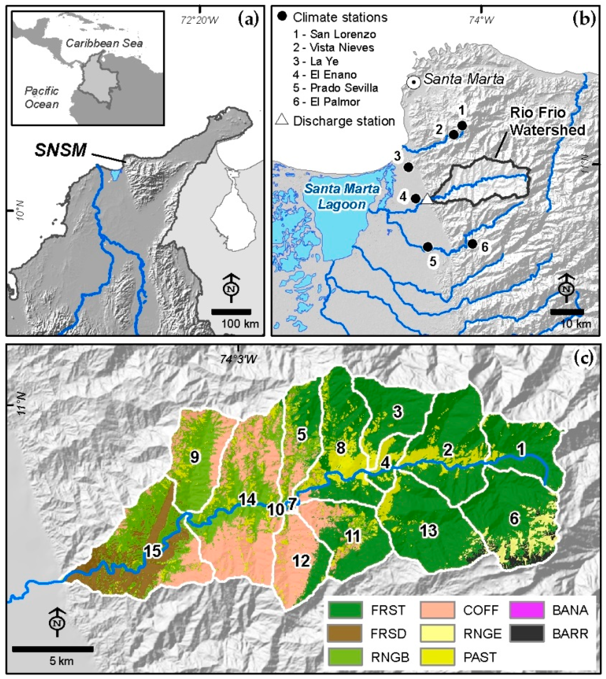
2.1. Study Site
2.2. Hydrologic Model
2.2.1. Data Sources and Processing
2.2.2. Model Setup
2.2.3. Model Calibration and Validation
- Step 1, Data quality assurance and control. Daily observed values of stream discharge were screened for quality. Values that were both quality-flagged and considered outliers were removed from the record, and remaining values used to construct monthly discharge for use in simulation and analysis.
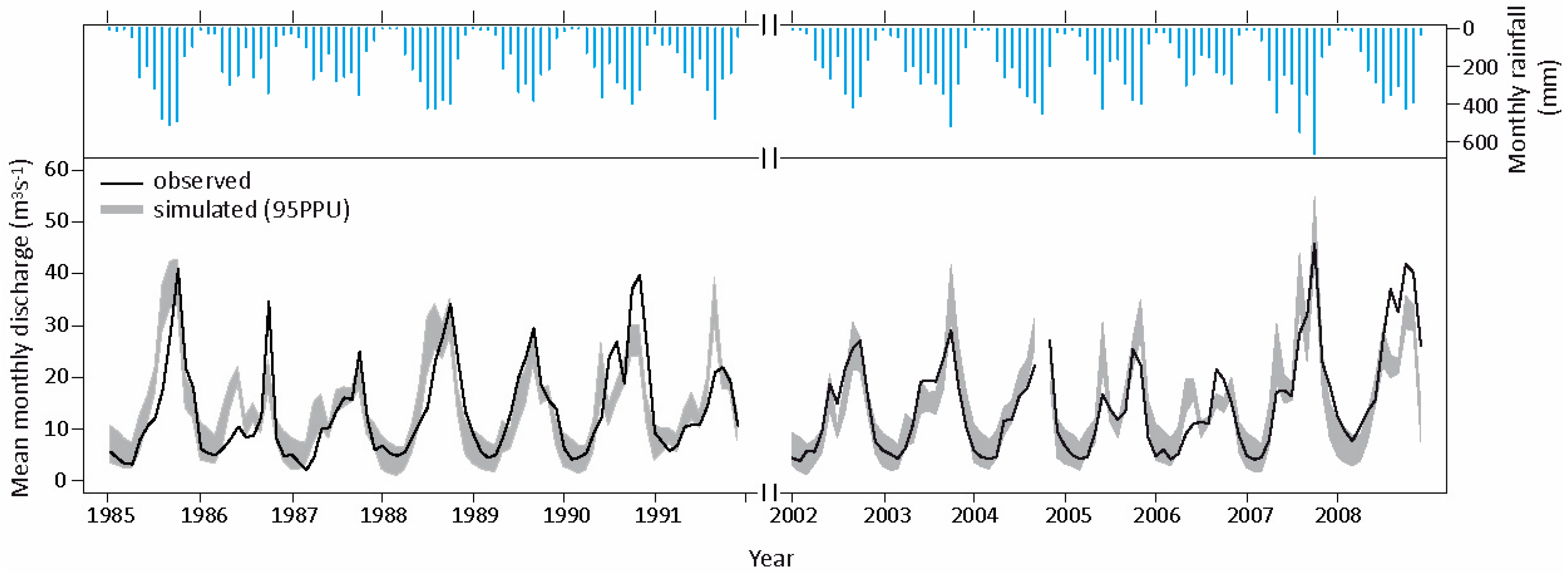
- Step 2, Simulation period definition. We selected calibration and validation periods that included wet, average and dry years, and had a relatively low number of quality flags. Accordingly, we defined 2002–2008 as the calibration period, with a three-year warm-up from 1999–2001, and 1985–1991 as the validation period, with a three-year warm-up from 1982–1984.
- Step 3, Determination of flow-path goals. To identify aspects of the modeled flow paths that needed improvement (hereafter, “flow-path goals”), we performed an initial comparison of literature-based observations to the following outputs from SWAT in its default configuration: fraction of total runoff as baseflow, calculated from daily discharge using a baseflow filter (https://engineering.purdue.edu/mapserve/WHAT/), ratios of total ET/total precipitation and surface runoff/total streamflow as measured in the central Colombian Andes [48,49,50]. Based on this comparison, we determined that the calibration process should, relative to SWAT defaults, decrease total runoff and increase total baseflow and ET.
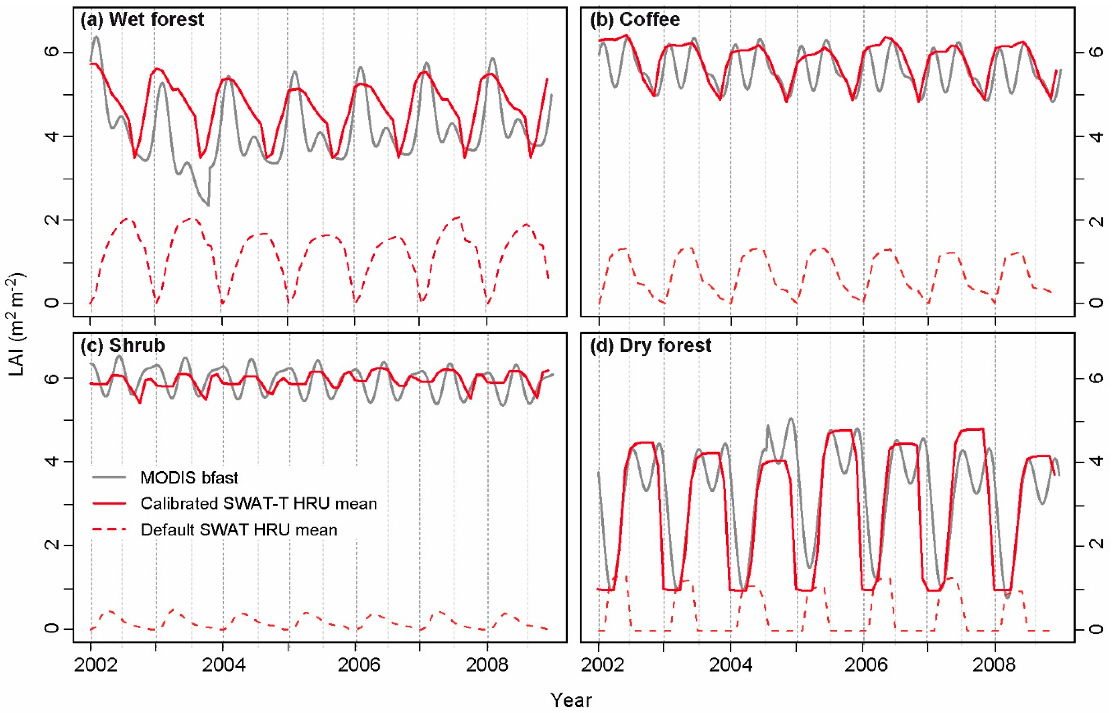
- Step 4, SWAT calibration of LAI. We found that the default configuration of SWAT provided a poor representation of LAI dynamics. We therefore calibrated SWAT-simulated LAI to MODIS-derived, eight-day LAI composites using the SWAT-T module for tropical vegetation growth [51,52]. This SWAT module has been shown to improve the representation of shifts between vegetation dormancy and growth in tropical regions by using soil moisture, rather than day-length, to represent important phenological thresholds. For more information, see Supplementary Materials S3.
- Step 5, Sensitivity analysis. To identify important model parameters to estimate via calibration, we performed a global sensitivity analysis of monthly simulated streamflow to 16 selected parameters. This was done by ranking trend p-values for each parameter in question, with other parameters varying simultaneously, using 500 simulations in SWAT-CUP. We selected the 10 most influential parameters (listed in Supplementary Materials S4) to estimate via calibration. During the calibration process described next, we also performed local, one-at-time sensitivity analyses to select initial parameter ranges for SUFI-2 calibration that were compatible with our flow-path goals (Step 3, Supplementary Materials S5).
- Step 6, Calibration. We calibrated monthly streamflow with SUFI-2 using 1000 simulations per iteration (latin hypercube sampling) and the Nash–Sutcliffe (NS) coefficient as the “goal function” for suggested parameter range-centering. We manually limited parameter ranges input to SUFI-2 by considering our flow-path goals (Step 3), uncertainty statistics (p-value and r-value) [45,46], and performance criteria [53]. This was done by repeating Steps 5 and 6 on a trial-and-error basis until acceptable values were attained.
- Step 7, Validation. Once we obtained satisfactory calibration results, we tested the model against streamflow using the parameter ranges obtained from calibration (steps 4 and 6).
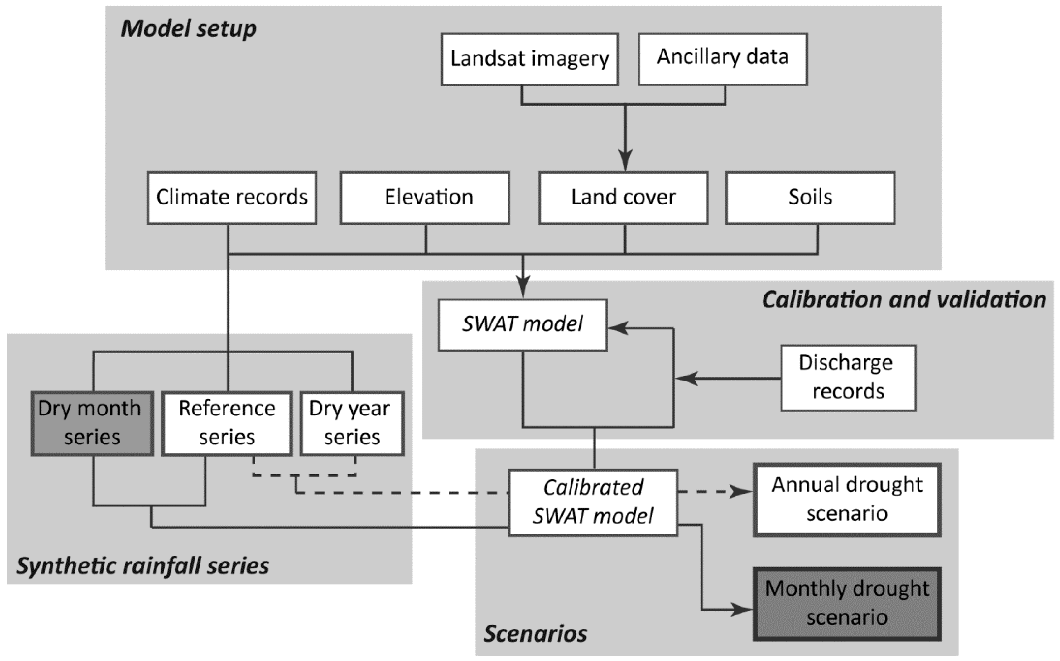
2.3. Scenarios
2.3.1. Synthetic Rainfall Series
2.3.2. HRU Selection
2.3.3. Statistical Analyses
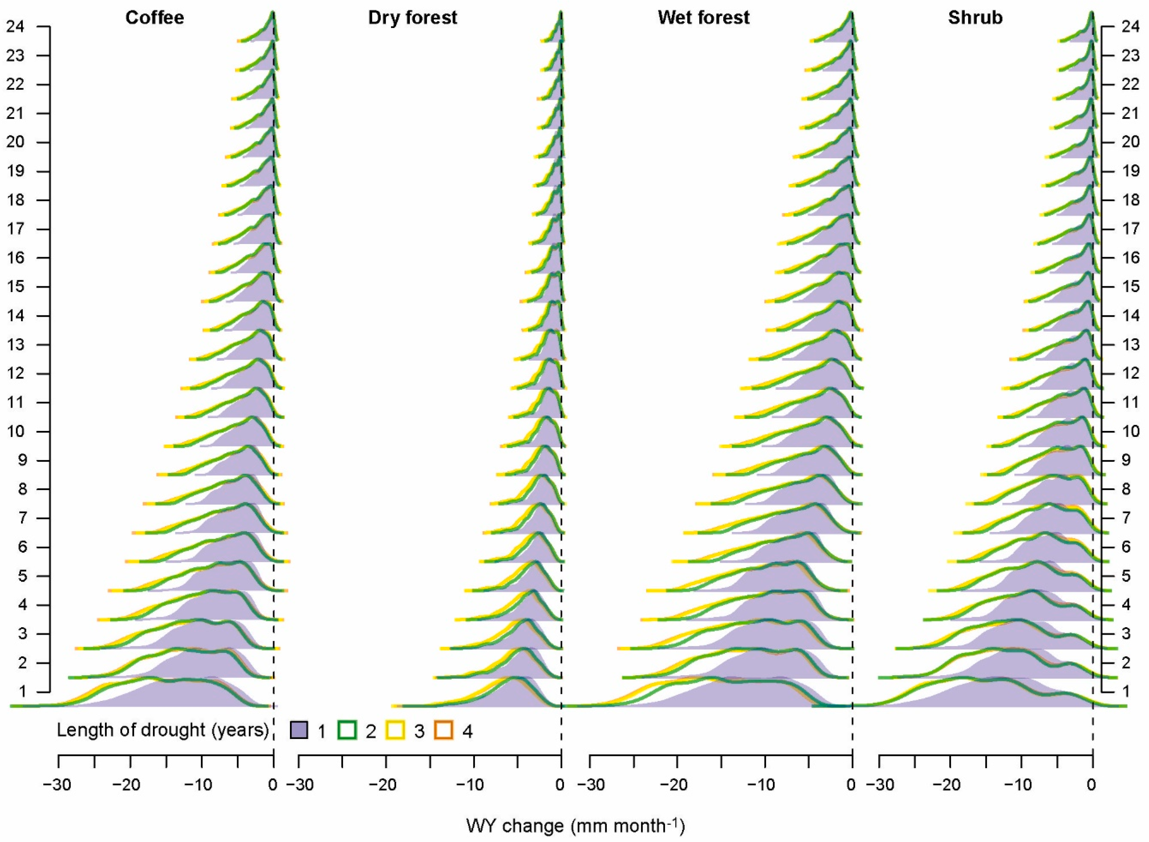
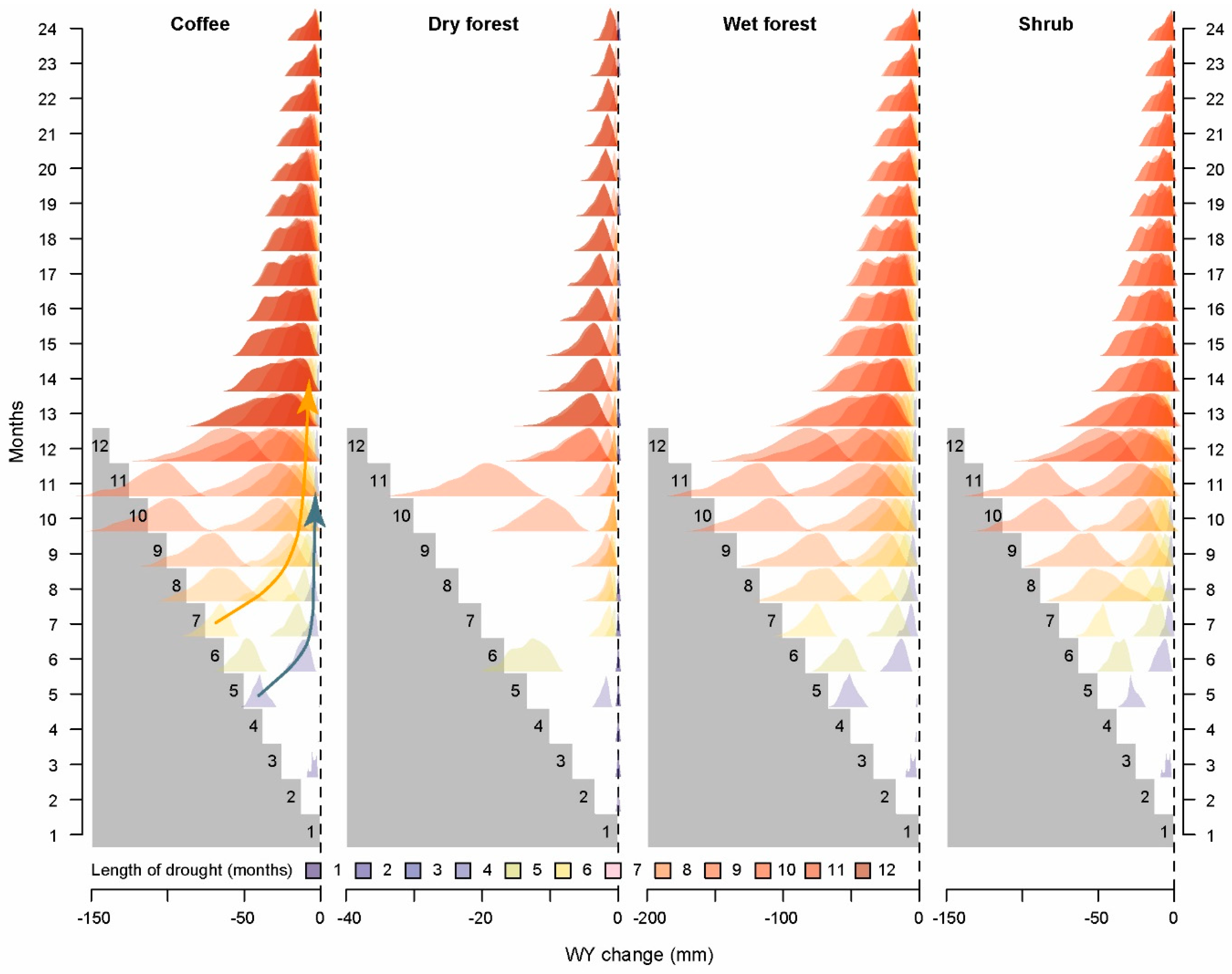
- Water yield recovery time after drought termination: For each selected HRU, we plotted PDFs starting in month 1 after drought termination.
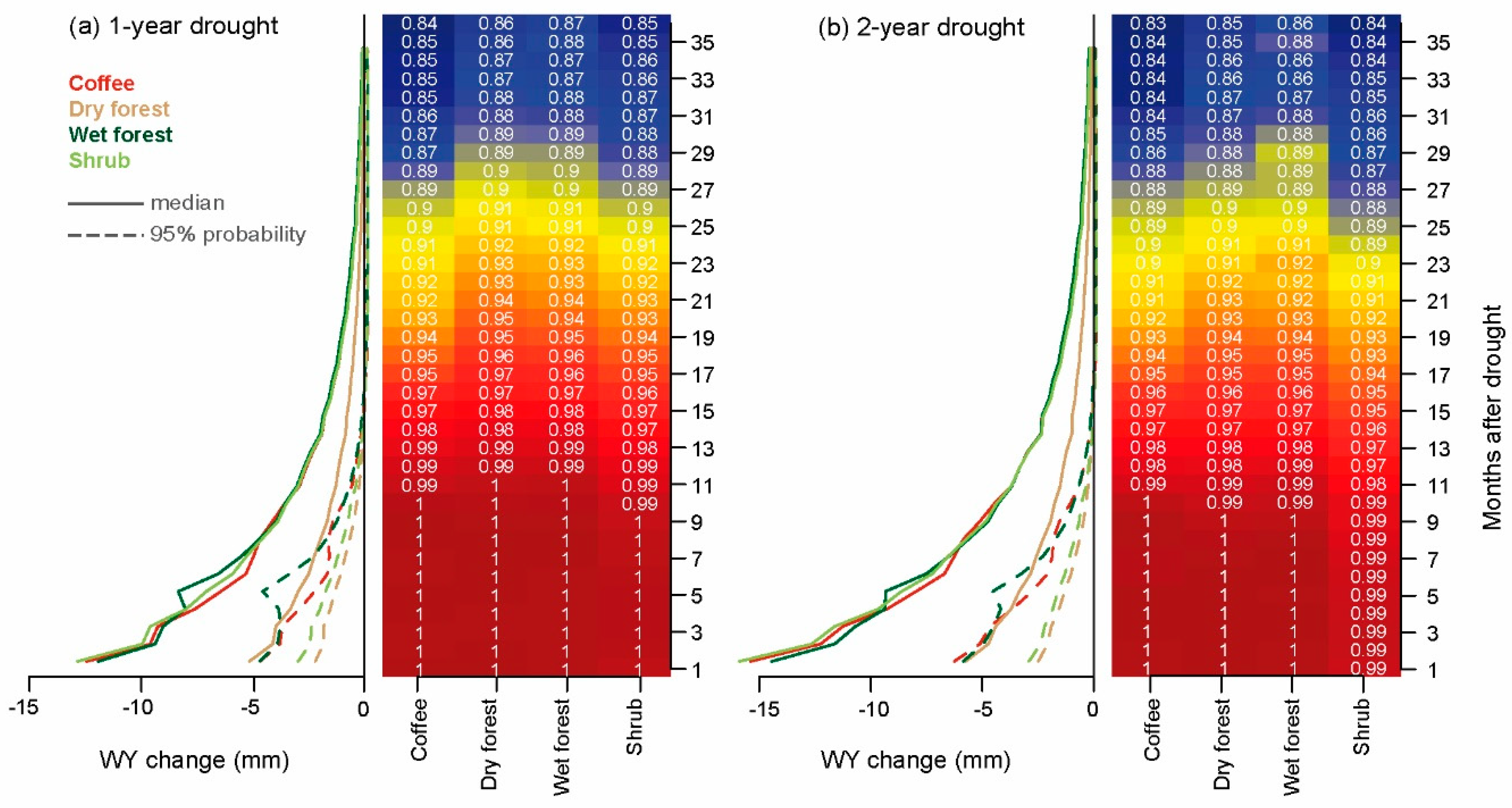
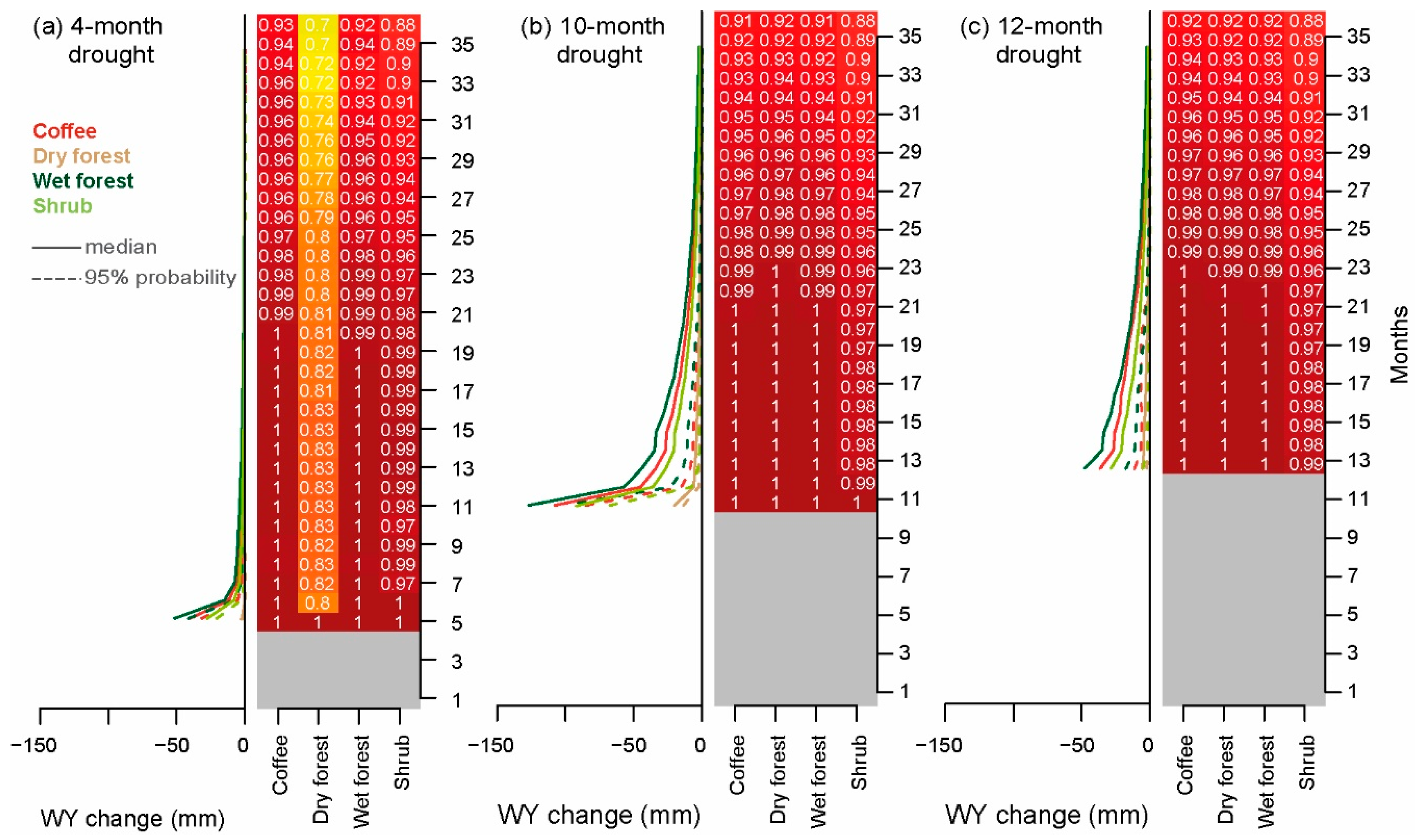
- Water yield decrease magnitude as indicated by the PDF median value for each month/scenario (value of water yield decrease that divides the area under the PDF in half).
- Probability of water yield decrease measured as the area under the PDF and to the left of zero. It is worth mentioning that high probabilities of water yield reduction do not necessarily imply a severe reduction (i.e., high probability can be associated with low magnitude).
3. Results
3.1. Land Cover Classification
3.2. SWAT-T leaf Area Index (LAI) Calibration
3.3. Discharge Calibration and Validation
3.4. Scenarios
3.4.1. Annual Drought Scenarios
3.4.2. Monthly Drought Scenarios
4. Discussion
4.1. Drought Propagation
4.2. Land Cover Effects
5. Conclusions
Supplementary Materials
Author Contributions
Funding
Acknowledgments
Conflicts of Interest
References
- Steffen, W.; Persson, A.; Deutsch, L.; Zalasiewicz, J.; Williams, M.; Richardson, K.; Crumley, C.; Crutzen, P.; Folke, C.; Gordon, L.; et al. The anthropocene: From global change to planetary stewardship. Ambio 2011, 40, 739–761. [Google Scholar] [CrossRef] [PubMed]
- IPCC. Climate Change 2007: The Physical Science Basis; Cambridge University Press: Cambridge, UK, 2007; p. 987. [Google Scholar]
- FAO. AQUASTAT. Available online: http://www.fao.org/nr/water/aquastat/countries_regions/americas/indexesp3.stm (accessed on 3 October 2018).
- Nurse, L.A.; Sem, G.; Hay, J.E.; Suarez, A.G.; Wong, P.P.; Briguglio, L.; Ragoonaden, S. Small island states. In Climate Change 2001: Impacts, Adaptation, and Vulnerability; McCarthy, J.J., Canziani, O.F., Leary, N.A., Dokken, D.J., White, K.S., Eds.; Cambridge University Press: Cambridge, UK, 2001; pp. 843–875. [Google Scholar]
- Neelin, J.D.; Münnich, M.; Su, H.; Meyerson, J.E.; Holloway, C.E. Tropical drying trends in global warming models and observations. Proc. Natl. Acad. Sci. USA 2006, 103, 6110–6115. [Google Scholar] [CrossRef] [PubMed] [Green Version]
- Campbell, J.D.; Taylor, M.A.; Stephenson, T.S.; Watson, R.A.; Whyte, F.S. Future climate of the Caribbean from a regional climate model. Int. J. Climatol. 2011, 31, 1866–1878. [Google Scholar] [CrossRef]
- Singh, B. Climate changes in the greater and southern Caribbean. Int. J. Climatol. 1997, 17, 1093–1114. [Google Scholar] [CrossRef] [Green Version]
- Angeles, M.E.; Gonzalez, J.E.; Erickson, D.J.I.; Hernandez, J.L. Predictions of future climate change in the Caribbean region using global general circulation models. Int. J. Climatol. 2006, 27, 555–569. [Google Scholar] [CrossRef]
- Herrera, D.A.; Ault, T.R.; Fasullo, J.T.; Coats, S.J.; Carrillo, C.M.; Cook, B.I.; Williams, A.P. Exacerbation of the 2013–2016 Pan-Caribbean Drought by Anthropogenic Warming. Geophys. Res. Lett. 2018, 45, 10619–10626. [Google Scholar] [CrossRef]
- Van Loon, A.F. Hydrological drought explained. Wiley Interdiscip. Rev. Water 2015, 2, 359–392. [Google Scholar] [CrossRef] [Green Version]
- Van Lanen, H.A.J.; Wanders, N.; Tallaksen, L.M.; Van Loon, A.F. Hydrological drought across the world: Impact of climate and physical catchment structure. Hydrol. Earth Syst. Sci. 2013, 17, 1715–1732. [Google Scholar] [CrossRef]
- Van Loon, A.F.; Gleeson, T.; Clark, J.; Van Dijk, A.I.J.M.; Stahl, K.; Hannaford, J.; Di Baldassarre, G.; Teuling, A.J.; Tallaksen, L.M.; Uijlenhoet, R.; et al. Drought in the Anthropocene. Nat. Geosci. 2016, 9, 89–91. [Google Scholar] [CrossRef] [Green Version]
- Van Loon, A.F.; Tijdeman, E.; Wanders, N.; Van Lanen, H.A.J.; Teuling, A.J.; Uijlenhoet, R. How climate seasonality modifies drought duration and deficit. J. Geophys. Res. Atmos. 2014, 119, 4640–4656. [Google Scholar] [CrossRef] [Green Version]
- Aldana-Domínguez, J.; Montes, C.; Martínez, M.; Medina, N.; Hahn, J.; Duque, M. Biodiversity and ccosystem services knowledge in the Colombian Caribbean: Progress and challenges. Trop. Conserv. Sci. 2017, 10, 1940082917714229. [Google Scholar] [CrossRef]
- Tribin, M.C.D.G.; Rodriguez, N.G.E.; Valderrama, M. Sierra Nevada de Santa Marta: A Pioneer Experience of a Shared and Coordinated Management of a Bioregion; UNESCO: Paris, France, 1999; p. 40. [Google Scholar]
- Ruiz, F.; Rodriguez, A.; Armenta, G.; Grajales, F. Informe de Escenarios de Cambio Climático para Temperatura y Precipitación en Colombia; IDEAM: Bogotá, Colombia, 2013; p. 81.
- IDEAM; PNUD; MADS; DNP; CANCILLERÍA. Escenarios de Cambio Climático para Precipitación y Temperatura para Colombia 2011–2100: Herramientas Científicas para la Toma de Decisions—Estudio Técnico Completo: Tercera Comunicación Nacional de Cambio Climático; IDEAM: Bogotá, Colombia, 2015; p. 278.
- Ochoa, A.; Poveda, G. Distribución espacial de señales de cambio climático en Colombia. In Proceedings of the XXIII Congreso Latinoamericano de Hidráulica, Cartagena, Colombia, 2–6 September 2008. [Google Scholar]
- Cantor, D.C. Evaluación y Análisis Espacio Temporal de Tendencias de Largo plazo en la Hidroclimatología Colombiana; Universidad Nacional de Colombia: Medellín, Colombia, 2011. [Google Scholar]
- Pabón, J.D. Cambio climático en Colombia: Tendencias en la segunda mitad del siglo XX y escenarios posibles para el siglo XXI. Rev. Acad. Colomb. Cienc. Exactas Fís. Nat. 2012, 36, 261–278. [Google Scholar]
- Carmona, A.M.; Poveda, G. Detection of long-term trends in monthly hydro-climatic series of Colombia through Empirical Mode Decomposition. Clim. Chang. 2014, 123, 301–313. [Google Scholar] [CrossRef]
- Hurtado, A.F.; Mesa, O.J. Cambio climático y variabilidad espacio-temporal de la precipitación en Colombia. Rev. EIA 2015, 12, 131–150. [Google Scholar] [CrossRef]
- Pierini, J.O.; Restrepo, J.C.; Aguirre, J.; Bustamante, A.M.; Velásquez, G.J. Changes in seasonal streamflow extremes experienced in rivers of Northwestern South America (Colombia). Acta Geophys. 2017, 65, 377–394. [Google Scholar] [CrossRef] [Green Version]
- UNGRD. Fenómeno El Niño. Análisis Comparativo 1997–1998//2014–2016; Unidad Nacional para la Gestión del Riesgo de Desastres: Bogotá, Colombia, 2016; p. 143.
- Restrepo, J.C.; Ortiz, J.C.; Pierini, J.; Schrottke, K.; Maza, M.; Otero, L.; Aguirre, J. Freshwater discharge into the Caribbean Sea from the rivers of Northwestern South America (Colombia): Magnitude, variability and recent changes. J. Hydrol. 2014, 509, 266–281. [Google Scholar] [CrossRef]
- International Global Atmospheric Chemistry (IGAC). Estudio General de suelos y Zonificación del Tierras: Departamento del Magdalena, Escala 1:100000; IGAC: Bogotá, Colombia, 2009.
- Fundación Pro-Sierra Nevada de Santa Marta. Plan de Desarrollo Sostenible de la Sierra Nevada de Santa Marta; Fundación Pro-Sierra Nevada de Santa Marta: Santa Marta, Colombia, 1997; p. 228. [Google Scholar]
- Uribe, E. Natural Resource Conservation and Management in the Sierra Nevada of Santa Marta: Case Study; Universidad de los Andes: Bogotá, Colombia, 2005. [Google Scholar]
- MADS; IDEAM; IAvH; INVEMAR; IIAP; SINCHI; PNN; IGAC. Mapa de Ecosistemas Continentales, Costeros y Marinos de Colombia Version 1.0; IDEAM: Bogotá, Colombia, 2015.
- IDEAM (Instituto de Hidrología, Meteorología y Estudios Ambientales). Informe del Estado de los Glaciares Colombianos; Instituto de Hidrología, Meteorología y Estudios Ambientales: Bogotá, Colombia, 2018.
- Neitsch, S.L.; Arnold, J.G.; Kiniry, J.R.; Williams, J.R. Soil and Water Assessment Tool Theoretical Documentation, Version 2009; Texas Water Resources Institute: College Station, TX, USA, 2011; p. 618. [Google Scholar]
- Arnold, J.G.; Moriasi, D.N.; Gassman, P.W.; Abbaspour, K.C.; White, M.J.; Srinivasan, R.; Santhi, C.; Harmel, R.D.; van Griensven, A.; Van Liew, M.W.; et al. SWAT: Model use, calibration, and validation. Trans. ASABE 2012, 55, 1491–1508. [Google Scholar] [CrossRef]
- Abe, C.A.; Lobo, F.L.; Dibike, Y.B.; Costa, M.P.F.; Dos Santos, V.; Novo, E.M.L.M. Modelling the effects of historical and future land cover changes on the hydrology of an Amazonian basin. Water 2018, 10, 932. [Google Scholar] [CrossRef]
- Montecelos-Zamora, Y.; Cavazos, T.; Kretzschmar, T.; Vivoni, E.R.; Corzo, G.; Molina-Navarro, E. Hydrological modeling of climate change impacts in a tropical river basin: A case study of the Cauto river, Cuba. Water 2018, 10, 1135. [Google Scholar] [CrossRef]
- QGIS Development Team. QGIS Geographic Information System; Open Source Geospatial Foundation Project, 2.18.6; QGIS Development Team, 2017. [Google Scholar]
- Saxton, K.E.; Rawls, W.J. Soil water characteristic estimates by texture and organic matter for hydrologic solutions. Soil Sci. Soc. Am. J. 2006, 70, 1569–1578. [Google Scholar] [CrossRef]
- Borselli, L. KUERY. Global Erodibility Database Query, 1.4; San Luis Potosí, Mexico, 2013. [Google Scholar]
- Borselli, L.; Torri, D.; Poesen, J.; Iaquinta, P. A robust algorithm for estimating soil erodibility in different climates. Catena 2012, 97, 85–94. [Google Scholar] [CrossRef]
- Post, D.F.; Fimbres, A.; Matthias, A.D.; Sano, E.E.; Accioly, L.; Batchily, A.K.; Ferreira, L.G. Predicting soil albedo from soil color and spectral reflectance data. Soil Sci. Soc. Am. J. 2000, 64, 1027–1034. [Google Scholar] [CrossRef]
- Breiman, L. Random forests. Mach. Learn. 2001, 45, 5–32. [Google Scholar] [CrossRef]
- Chavez, P.S. Image-based atmospheric corrections—Revisited and improved. Photogramm. Eng. Remote Sens. 1996, 62, 1025–1036. [Google Scholar]
- R Core Team R: A Language and Environment for Statistical Computing; R Foundation for Statistical Computing: Vienna, Austria, 2017.
- Breiman, L.; Cutler, A. Random Forests. Available online: https://www.stat.berkeley.edu/~breiman/RandomForests/cc_home.htm (accessed on 10 February 2016).
- Myneni, R.; Knyazikhin, Y.; Park, T. MOD15A2H MODIS/Terra Leaf Area Index/FPAR 8-Day L4 Global 500m SIN Grid V006; NASA EOSDIS Land Processes DAAC: Sioux Falls, SD, USA, 2015.
- Abbaspour, K.C.; Johnson, C.A.; van Genuchten, M.T. Estimating Uncertain Flow and Transport Parameters Using a Sequential Uncertainty Fitting Procedure. Vadose Zone J. 2004, 3, 1340–1352. [Google Scholar] [CrossRef]
- Abbaspour, K.C.; Yang, J.; Maximov, I.; Siber, R.; Bogner, K.; Mieleitner, J.; Zobrist, J.; Srinivasan, R. Modelling hydrology and water quality in the pre-alpine/alpine Thur watershed using SWAT. J. Hydrol. 2007, 333, 413–430. [Google Scholar] [CrossRef]
- Abbaspour, K.C.; Srinivasan, R. SWAT-CUP, 5.1.6.2; EAWAG: Dubendorf, Switzerland, 2013. [Google Scholar]
- Suárez de Castro, F.; Rodríguez Grandas, A. Investigaciones Sobre la Erosión y la Conservación de los Suelos en Colobia; Federación Nacional de Cafeteros: Bogotá, Colombia, 1962; p. 471. [Google Scholar]
- Jaramillo-Robledo, A. El balance hídrico. In Clima andino y café en Colombia; Cenicafé: Chinchiná, Colombia, 2005; pp. 107–123. [Google Scholar]
- García-Leoz, V.; Villegas, J.C.; Suescún, D.; Flórez, C.P.; Merino-Martín, L.; Betancur, T.; León, J.D. Land cover effects on water balance partitioning in the Colombian Andes: Improved water availability in early stages of natural vegetation recovery. Reg. Environ. Chang. 2018, 18, 1117–1129. [Google Scholar] [CrossRef]
- Strauch, M.; Volk, M. SWAT plant growth modification for improved modeling of perennial vegetation in the tropics. Ecol. Model. 2013, 269, 98–112. [Google Scholar] [CrossRef]
- Alemayehu, T.; van Griensven, A.; Woldegiorgis, B.T.; Bauwens, W. An improved SWAT vegetation growth module and its evaluation for four tropical ecosystems. Hydrol. Earth Syst. Sci. 2017, 21, 4449–4467. [Google Scholar] [CrossRef] [Green Version]
- Moriasi, D.N.; Arnold, J.G.; Van Liew, M.W.; Bingner, R.L.; Harmel, R.D.; Veith, T.L. Model evaluation guidelines for systematic quantification of accuracy in watershed simulations. Trans. ASABE 2007, 50, 885–900. [Google Scholar] [CrossRef]
- Arnold, J.G.; Kiniry, J.R.; Srinivasan, R.; Williams, J.R.; Haney, E.B.; Neitsch, S.L. SWAT Input/Output Documentation, Version 2012; Texas Water Resources Institute: College Station, TX, USA, 2012; p. 654. [Google Scholar]
- Van Loon, A.F.; Van Lanen, H.A.J. A process-based typology of hydrological drought. Hydrol. Earth Syst. Sci. 2012, 16, 1915–1946. [Google Scholar] [CrossRef] [Green Version]
- Van Loon, A.F.; Laaha, G. Hydrological drought severity explained by climate and catchment characteristics. J. Hydrol. 2015, 526, 3–14. [Google Scholar] [CrossRef] [Green Version]
- Wohl, E.; Barros, A.; Brunsell, N.; Chappell, N.A.; Coe, M.; Giambelluca, T.; Goldsmith, S.; Harmon, R.; Hendrickx, J.M.H.; Juvik, J.; et al. The hydrology of the humid tropics. Nat. Clim. Chang. 2012, 2, 655. [Google Scholar] [CrossRef]
- Ogden, F.L.; Crouch, T.D.; Stallard, R.F.; Hall, J.S. Effect of land cover and use on dry season river runoff, runoff efficiency, and peak storm runoff in the seasonal tropics of Central Panama. Water Resour. Res. 2013, 49, 8443–8462. [Google Scholar] [CrossRef] [Green Version]
- Bruijnzeel, L.A. Hydrological functions of tropical forests: Not seeing the soil for the trees? Agric. Ecosyst. Environ. 2004, 104, 185–228. [Google Scholar] [CrossRef]
- Anderegg, W.R.L.; Konings, A.G.; Trugman, A.T.; Yu, K.; Bowling, D.R.; Gabbitas, R.; Karp, D.S.; Pacala, S.; Sperry, J.S.; Sulman, B.N.; et al. Hydraulic diversity of forests regulates ecosystem resilience during drought. Nature 2018, 561, 538–541. [Google Scholar] [CrossRef] [PubMed]
- Muñoz-Villers, L.E.; Holwerda, F.; Gómez-Cárdenas, M.; Equihua, M.; Asbjornsen, H.; Bruijnzeel, L.A.; Marín-Castro, B.E.; Tobón, C. Water balances of old-growth and regenerating montane cloud forests in central Veracruz, Mexico. J. Hydrol. 2012, 462–463, 53–66. [Google Scholar] [CrossRef]
- Muñoz-Villers, L.E.; McDonnell, J.J. Land use change effects on runoff generation in a humid tropical montane cloud forest region. Hydrol. Earth Syst. Sci. 2013, 17, 3543–3560. [Google Scholar] [CrossRef] [Green Version]
- Cavelier, J.; Aide, T.M.; Santos, C.; Eusse, A.M.; Dupuy, J.M. The Savannization of Moist Forests in the Sierra Nevada de Santa Marta, Colombia. J. Biogeogr. 1998, 25, 901–912. [Google Scholar] [CrossRef]
- Ponette-González, A.G.; Weathers, K.C.; Curran, L.M. Water inputs across a tropical montane landscape in Veracruz, Mexico: Synergistic effects of land cover, rain and fog seasonality, and interannual precipitation variability. Glob. Chang. Biol. 2010, 16, 946–963. [Google Scholar] [CrossRef]
- Jaramillo-Robledo, A.; Cháves-Córdoba, B. Aspectos hidrológicos en un bosque y en plantaciones de café (Coffea arabica L.) al sol y bajo sombra. Cenicafé 1999, 50, 97–105. [Google Scholar]


| Data | Source 1 | Relevant Characteristics |
|---|---|---|
| Elevation | IGAC | 1:25,000 scale |
| Soil mapping units | [29] | 1:100,000 scale |
| Soil properties | [26] | Soil profiles from state´s soil survey |
| Land cover | Landsat 8 image from 11 January 2015 | 30 m spatial resolution |
| Leaf area index | MODIS LAI products MOD15A2Hv006 (January 2002–June 2002) MCD15A2Hv006 (July 2002–December 2008) [44] | 500 m spatial resolution, 8-day composites |
| Precipitation | IDEAM | Total daily precipitation |
| Daily maximum and minimum temperature | IDEAM | Maximum and minimum daily temperature |
| Discharge | IDEAM | Average daily discharge Period 1968–2015 |
| Annual scenarios | Rainfall year 1 | ||||||||||||||||||
| 1 | 2 | 3 | 4 | 5 | 6 | 7 | |||||||||||||
| Reference | N | N | N | N | N | N | N | ||||||||||||
| Scen1 | D | N | N | N | N | N | N | ||||||||||||
| Scen2 | D | D | N | N | N | N | N | ||||||||||||
| Scen3 | D | D | D | N | N | N | N | ||||||||||||
| Scen4 | D | D | D | D | N | N | N | ||||||||||||
| Monthly scenarios | Rainfall month 1 | ||||||||||||||||||
| 1 | 2 | 3 | 4 | 5 | 6 | 7 | 8 | 9 | 10 | 11 | 12 | 13 to 84 | |||||||
| Reference | N | N | N | N | N | N | N | N | N | N | N | N | N | ||||||
| Scen1 | D | N | N | N | N | N | N | N | N | N | N | N | N | ||||||
| Scen2 | D | D | N | N | N | N | N | N | N | N | N | N | N | ||||||
| Scen3… | D | D | D | N | N | N | N | N | N | N | N | N | N | ||||||
| Scen12 | D | D | D | D | D | D | D | D | D | D | D | D | N | ||||||
| Modeling Period | Evaluation Statistics for Model Uncertainty | Evaluation Statistics for Best-Fit Simulation 1 | Performance Rating 2 | ||||
|---|---|---|---|---|---|---|---|
| p-factor | r-factor | NS 1 | PBIAS | RSR | R2 | ||
| Calibration (2002–2008) | 0.70 | 0.57 | 0.79 | 0.2 | 0.46 | 0.79 | Very good |
| Validation (1985–1991) | 0.71 | 0.60 | 0.72 | −3.4 | 0.53 | 0.73 | Good |
© 2019 by the authors. Licensee MDPI, Basel, Switzerland. This article is an open access article distributed under the terms and conditions of the Creative Commons Attribution (CC BY) license (http://creativecommons.org/licenses/by/4.0/).
Share and Cite
Hoyos, N.; Correa-Metrio, A.; Jepsen, S.M.; Wemple, B.; Valencia, S.; Marsik, M.; Doria, R.; Escobar, J.; Restrepo, J.C.; Velez, M.I. Modeling Streamflow Response to Persistent Drought in a Coastal Tropical Mountainous Watershed, Sierra Nevada De Santa Marta, Colombia. Water 2019, 11, 94. https://doi.org/10.3390/w11010094
Hoyos N, Correa-Metrio A, Jepsen SM, Wemple B, Valencia S, Marsik M, Doria R, Escobar J, Restrepo JC, Velez MI. Modeling Streamflow Response to Persistent Drought in a Coastal Tropical Mountainous Watershed, Sierra Nevada De Santa Marta, Colombia. Water. 2019; 11(1):94. https://doi.org/10.3390/w11010094
Chicago/Turabian StyleHoyos, Natalia, Alexander Correa-Metrio, Steven M. Jepsen, Beverley Wemple, Santiago Valencia, Matthew Marsik, Rubén Doria, Jaime Escobar, Juan C. Restrepo, and Maria I. Velez. 2019. "Modeling Streamflow Response to Persistent Drought in a Coastal Tropical Mountainous Watershed, Sierra Nevada De Santa Marta, Colombia" Water 11, no. 1: 94. https://doi.org/10.3390/w11010094